11	Diffraction
	Toru Yoshizawa

CONTENTS

11.1  Introduction

11.2  Fundamentals of Diffraction

11.3  Application of Diffractographic Method

11.4  Application of Grating Diffraction Method

11.5  Conclusion

References

11.1    INTRODUCTION

The diffraction phenomenon in which light sneaks around to the back of the shading screen is one of the typical properties inherent to light, and its physical explanation is described well in famous reference books on optics [1,2,3]. Diffraction is well known and we can easily observe this phenomenon by using a coherent beam from a laser. However, it is not easy to understand the theoretical description of diffraction completely. Here, we focus on diffraction in the Fraunhofer region, because it is much easier to understand fundamental properties of diffraction in this region rather than in the Fresnel region. In addition, most of the practical applications have been derived on the basis of the Fraunhofer diffraction. By using diffraction phenomena, a number of applications have been developed in optical metrology. However, topics such as structural analysis of a crystal using x-ray or neutron diffraction and another recently developed field like diffractive optics are not described here. The readers are referred to Refs. [4,5] to obtain useful knowledge in these fields.

11.2    FUNDAMENTALS OF DIFFRACTION

We start by using the famous and most fundamental expression called the Fresnel–Kirchhoff diffraction formula.

Let us consider the case of Figure 11.1 where an aperture is projected by a light (wavelength λ) from the source and the wave amplitude U_p is observed at the point P. To discuss the influence of this light through the aperture, we assume a domain S consisting of three regions S₁, S₂, and S₃ in Figure 11.1. We need to integrate the contribution from a small area dS over the domains S₁, S₂, and S₃. This domain S is enclosed by a screen S₂ (no contribution from this area, because the light amplitude does not exist), a semi-sphere S₃ with the observation point P at the center (also no contribution under the Sommerfeld radiation condition [2] although intuitive understanding is difficult and theoretical discussion is necessary in detail [3]), and the aperture S₁ which dominates the wave U_p at the point P.

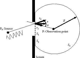
FIGURE 11.1  Derivation of Kirchhoff diffraction formula.

However, if we skip sophisticated discussion, the next equation called the Fresnel–Kirchhoff diffraction formula is obtained using wave number k =2π/λ (λ, wavelength) and amplitude A (a constant depending on the strength of the source)

$U_{\text{p}}=\frac{A}{j2\lambda }{\displaystyle \underset{S_1}{\int }\frac{\exp \left[jk\left(r_0+r_1\right)\right]}{r_0{r}_1}\left[\cos \left(r_1,n\right)-\cos \left(r_0,n\right)\right]\text{d}S}$

(11.1)

where the angle between unit vectors r₁ and n is (r₁, n) and the angle between r₀ and n is (r₀, n). This is called the Fresnel–Kirchhoff diffraction formula. Here, the factor [cos(r₁, n) − cos(r₀, n)] is introduced by Fresnel to overcome the difficulty (by Huygens’ construction) in explaining the direction of propagating light due to diffraction and is called the inclination factor.

If the light source is located far from the screen, cos(r₁, n) becomes unity, that is, cos(r₁, n) = 1, and let cos(r₀, n) be replaced by −cos χ (as shown in Figure 11.1). This assumption leads to the next expression:

$U_{\text{p}}=\frac{A}{j2\lambda }{\displaystyle \underset{S_1}{\int }\frac{\exp \left[jk\left(r_0+r_1\right)\right]}{r_0{r}_1}\left(1+\cos \chi \right)\text{d}S}$

(11.2)

Now the inclination factor is given by (1 + cos χ). In addition, if the observation point is far from the screen, this angle χ becomes nearly equal to zero (χ ≈ 0), and the inclination factor is approximated to be 2. This means that the amplitude is given by the following expression:

$U_{\text{p}}=\frac{A}{j\lambda }{\displaystyle \underset{S_1}{\int }\frac{\exp \left[jk\left(r_0+r_1\right)\right]}{r_0{r}_1}\text{d}S}$

(11.3)

However, except a limited number of cases, it is still difficult or impossible to solve the formula explicitly because of the integral term of the formula. For the purpose of understanding the diffraction to be applied to metrology, a further approximation is introduced to the formula.

In Figure 11.2, the aperture with the origin O is illuminated by the parallel uniformed beam from the source; then, g(x₀, y₀) plays the role of a light source on the aperture and it produces the diffracted pattern on the observing screen. One point P₀(x₀, y₀, 0) is located on the aperture plane, and the observing point P(x₁, y₁, z₁) is located on the screen. The distance P₀P is expressed by r and the distribution by U(x₁, y₁); then, the following equations hold

$U\left(x_1,y_1\right)=\frac{1}{j\lambda }{\displaystyle \underset{-\infty }{\overset{\infty }{\int }}{\displaystyle \int g\left(x_0,y_0\right)\frac{{\text{e}}^{jkr}}{r}\text{d}{x}_0\text{d}{y}_0}}$

(11.4)

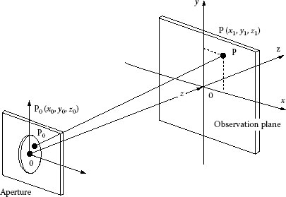
FIGURE 11.2  Diffraction due to aperture.

where

$r=\sqrt{z^2+{\left(x_0+x_1\right)}^2+{\left(y_0-y_1\right)}^2}$

(11.5)

However, this r makes the integration difficult.

If (x₀ − x₁)² + (y₀ − y₁)² is much smaller than z², that is, the screen is far from the aperture and the size of the aperture is not large, r is approximated as follows:

$r=z+\frac{x_1^2+y_1^2}{2z}-\frac{x_1{x}_0+y_1{y}_0}{z}+\frac{x_0^2+y_0^2}{2z}-\frac{{\left[{\left(x_1-x_0\right)}^2+{\left(y_1-y_0\right)}^2\right]}^2}{8z^3}$

(11.6)

In the case where the first three terms are used (the pattern is observed on the screen located far from the aperture), diffraction can be discussed in the Fraunhofer region, and if the first four terms are necessary (the pattern is observed on the screen near the aperture), we have to discuss the diffraction in the Fresnel region. In fact, mathematical considerations are extremely difficult regarding the Fresnel diffraction. Therefore, the Fraunhofer approximation is preferable for practical applications to metrology, that is, r is approximated by

$r=z+\frac{x_1^2+y_1^2}{2z}-\frac{x_1{x}_0+y_1{y}_0}{z}$

(11.7)

For example, when such a small aperture as 0.1 mm is illuminated by the beam with the wavelength λ= 0.63 μm, a distance longer than 60 mm is required; this is quite easy to realize. However, when a larger aperture with a size of 10 mm is illuminated, the distance has to be longer than 600 mm, which becomes difficult to realize. In this case, a convex lens is useful to observe a diffraction pattern in the Fraunhofer region [2]. The thickness of the convex lens (focal length f) decreases from the center to the rim in proportion to $\left(x_0^2+y_0^2\right)/2f$ , and this means the fourth term of Equation 11.6 can be canceled. Because, when the lens with the focal length f is inserted, z in Equation 11.6 is replaced by f and the fourth term is canceled by adding the phase $k\left(x_0^2+y_0^2\right)/2f$ .

Thus, the next equation is obtained

$U\left(x_1,y_1\right)=\frac{1}{j\lambda z}\exp \left[jk\left(z+\frac{x_1^2+y_1^2}{2z}\right)\right]{\displaystyle \underset{-\infty }{\overset{\infty }{\int }}{\displaystyle \int g\left(x_0,y_0\right)\exp \left[-j2\pi \left(\frac{x_1{x}_0+y_1{y}_0}{\lambda z}\right)\right]\text{d}{x}_0\text{d}{y}_0}}$

(11.8)

where r is also approximated by z in the denominator.

One application to metrology is suggested in Figure 11.3, where an aperture formed by two edgelike objects produces a diffraction pattern. If diffraction due to this aperture (with narrow width a)is observed on the screen located at the distance D (= z, far from the aperture), the pattern is formed in the Fraunhofer region. Thus, the Fresnel–Kirchhoff approximation, Equation 11.2 or 11.6, is expressed as follows. Here the aperture is given by

$\begin{array}{ll}U\left(x_1,y_1\right)\hfill & =\frac{1}{j\lambda z}\exp \left[jk\left(z+\frac{x_1^2+y_1^2}{2z}\right)\right]{\displaystyle \underset{-\infty }{\overset{\infty }{\int }}g\left(x_0\right)\exp \left[-j2\pi \left(\frac{x_1{x}_0}{\lambda z}\right)\right]\text{d}{x}_0}\hfill \\ \hfill & =\frac{1}{j\lambda z}\exp \left[jk\left(z+\frac{x_1^2+y_1^2}{2z}\right)\right]{\displaystyle \underset{-a/2}{\overset{a/2}{\int }}1\cdot \exp \left[-j2\pi \left(\frac{x_1{x}_0}{\lambda z}\right)\right]\text{d}x}\hfill \\ \hfill & =\frac{a}{\lambda z}\exp \left[jk\left(z+\frac{x_1^2+y_1^2}{2z}\right)\right]\cdot \sin c\left[\pi \left(\frac{a{x}_1}{\lambda z}\right)\right]\hfill \end{array}$

(11.9)

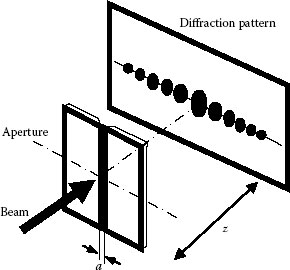
FIGURE 11.3  Diffraction pattern formed by two edges.

where

$g\left(x_0\right)=1\left(-a/2~a/2\right),0\left(\text{elsewhere}\right)$

In this case, calculation for integration is easily possible, but in most of the cases, this kind of mathematical calculation is nearly impossible. Therefore, the Fourier transformation method [6] should be used to know the diffraction pattern in the Fraunhofer region.

In the case of a rectangular aperture with the size of a × b, the next expression is easily guessed right:

$U\left(x_1,y_1\right)=\frac{ab}{j\lambda z}\exp \left[jk\left(z+\frac{x_1^2+y_1^2}{2z}\right)\right]\sin c\left(\pi \frac{a{x}_1}{\lambda z}\right)\sin c\left(\pi \frac{b{y}_1}{\lambda z}\right)$

(11.10)

Beautiful photographs of diffraction patterns brought by various shapes of apertures are represented in books with other pictures of interference and polarization [7,8].

Coming back to Figure 11.3, let us remove the suffix from x₁ to make it a simple expression and let the amplitude be expressed as I(x), which is given by |U(x)|².

Equation 11.7 indicates that the intensity distribution I(x) of the diffraction pattern is dominated by the function $\sin c\left(\pi \frac{ax}{\lambda Z}\right)$ . The profiles of the amplitude and intensity distributions are represented in Figure 11.4a and b. We should note that the dark points appear at the points $x=\frac{\lambda z}{a},2\frac{\lambda z}{a},3\frac{\lambda z}{a},4\frac{\lambda z}{a}$ , etc. with the equal interval $\text{Δ\hspace{0.17em}}=\frac{\lambda z}{a}$ , but the interval between the adjacent two bright points is not exactly equal, as shown in Table 11.1, where z is replaced by f because a lens is usually placed near the aperture to realize the Fraunhofer diffraction.

Therefore, if this interval Δ could be known, the gap (aperture size) a between two edges can be calculated by

$a=\frac{\lambda z}{\text{Δ}}$

(11.11)

Instead of detecting the darkest points, Δ defined by the bright points are also used. Naturally, this Δ is not constant near the central part of the diffraction pattern (in low diffraction order area); then, spots with higher orders of diffraction should be used.

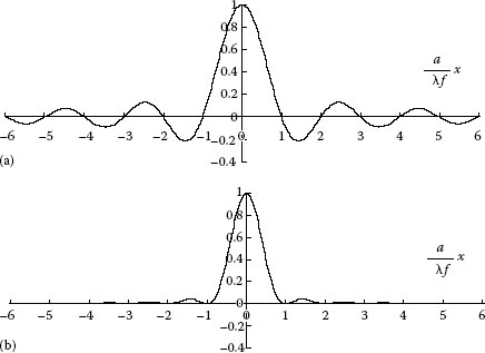
FIGURE 11.4  Distribution profile of a diffraction pattern of a slit aperture: (a) amplitude and (b) intensity.

A kind of tensile strength testing is proposed in Ref. [9] where L-shaped metal edges (at low temperature) or ceramic edges (at high temperature) are attached to a specimen for measuring the strain caused by loading. An aperture and its change formed between opposing edges brings diffraction, and strain is derived from the resultant pattern.

TABLE 11.1 Maximum Values of Intensity Curve

$\frac{a}{\lambda f}x$	1.4306	2.4583	3.4722	4.4778	5.4806
I	0.0472	0.0165	0.0083	0.0050	0.0034
$\frac{a}{\lambda f}x$	6.4833	7.4861	8.4889	9.4889	10.4917
I	0.0024	0.0018	0.0014	0.0011	0.0009

As another application, let us consider one example in which the diameter of a thin wire can be measured using diffraction phenomenon. Nowadays, an optical micrometer is introduced in a textbook on precision measurement of length, and the fundamental principle dates back to the 1920s. At that time, a mercury lamp was used for these experiments, but now with a laser source we can easily confirm this principle.

As shown in Figure 11.5, when such a thin line is projected by a laser beam, we can observe a diffraction pattern, shown in Figure 11.6, on the screen off the distance f from the lens (with the focal length f), which is placed close to the slit. Here, we should note the fact that a diffraction pattern caused by an aperture is exactly the same (except the neighborhood of the optical axis in the Fraunhofer region) as that formed by a mask of the same size and shape. This is explained on the basis of Babinet’s principle (see Ref. [4, p. 424]). Here, the equi-linear interval of the pattern on the screen is proportional to the slit-screen distance, that is, the focal length f of the lens is placed close to the slit. The linear distance d between successive minima Δ = fλ/d is exactly the same, but the distance between successive maxima is not constant. We should note that the detection of the minimum point is practically impossible, that is, we are required to find the brightest points. Fortunately, we can use the same equation Δ = fλ/d (now Δ denotes the distance between two successive bright spots), because the brightest spots are equally spaced in the higher-order region of diffraction. Thus, the separation Δ of the higher orders of bright spots is available to determine the diameter d of the wire. Moreover, we should note that the accuracy of measurement becomes higher as the diameter of the wire becomes smaller, because the separation is larger in inverse proportion to the diameter. The result of the measurement by this method is shown in Figure 11.7 together with results using two other methods: a toolmaker’s microscope and a mechanical micrometer.

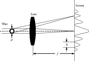
FIGURE 11.5  Diameter measurement of a thin wire.

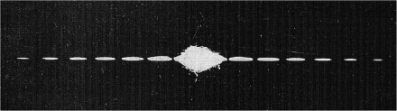
FIGURE 11.6  Diffraction pattern by an enamel wire.

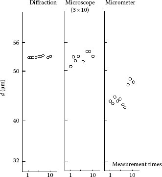
FIGURE 11.7  Measurement of an enamel wire.

The results of 10 times the measurements of an enamel wire by a beginner are shown in Figure 11.7, where repeatability using the diffraction method brought better results than the two other methods. In the case of a micrometer, the diameter measured is smaller due to contact force, and in the case of the microscopic measurement, the averaged value is nearly the same as that with the diffraction method, but the respective result varies widely. On the contrary, the diffraction method brings high repeatability and correct result. In an industrial application of this method, a thin enamel wire with a diameter of 0.1 to ~0.01 mm is inspected during running for winding onto a reel. A thin wire with an outer diameter of 30 ± 4 μm can be measured at the repeatability of 0.05 μm without any influence of vibration while running. One important fact is that the intensity distribution of the diffraction pattern is stationary, even if the objective vibrates, as long as it remains inside the beam spot. As stated earlier, the line object produces the same diffraction pattern with the slit aperture.

11.3    APPLICATION OF DIFFRACTOGRAPHIC METHOD

Displacement and profile are also easily measured using changes in diffraction pattern, which are caused by a clearance between a sample and the reference. Especially, if the resulting pattern is captured in the Fraunhofer region, a simple calculation is applicable. This kind of technique is named “diffractography,” and many practical applications of this technique have been reported [9,10].

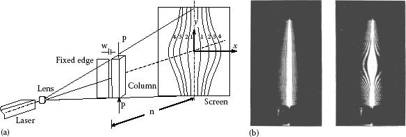
FIGURE 11.8  Diffraction pattern formed by deformation of a column. (a) Optical arrangement and (b) photographed pattern. (After Pryor, T.R. et al., Appl. Optics, 11(2), 314, 1972.)

By this technique, the measurement of displacement, especially displacements of a sample object along a line, is easily attainable. Line measurements of displacement are possible at all points along the reference line, with high accuracies over a large range and at one point.

Typically, let us consider Figure 11.8a, which shows the measurement of the slit aperture or change in the aperture formed between the reference edge and the test object. This arrangement is applicable to measure the deflection of a loaded column. Two diffracted patterns are shown in the figure (noises are caused by surface irregularities of the column), and the two results are represented in Figure 11.8b, where a small curvature of the column is detected (in comparison with the straight edge) when not loaded (left) and when loaded (right). This result is brought by the deflection due to a loading of 18.2 kg (178.4 N).

In Figure 11.9, the dynamic accuracy of a tool in ultrasonic welding is checked by this method [12]. In this case, the tool attached to an ultrasonic horn vibrates back and forth and around (Figure 11.9a), and when an aperture between a knife-edge and the tool gives a diffraction pattern (Figure 11.9b and c). We can observe the vibrating characteristics of the tool, and at the same time we can find signs of deterioration of the tool.

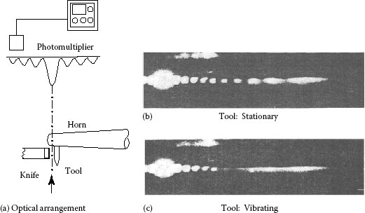
FIGURE 11.9  Vibration analysis of ultrasonic welding tool: (a) optical arrangement and (b and c) diffraction patterns. (From Ono, A. and Komatsu, T., Bull. Jpn. Soc. Precision Eng., 11(2), 101, 1977. With permission.)

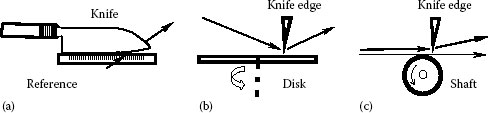
FIGURE 11.10  Some applications of diffractographic method. (a) Blade check of a knife. (b) Bounce of a rotary table. (c) Runout of a rotary shaft.

When the tool vibrates, the pattern and visibility of the fringe change, and transitional vibration as well as amplitude are analyzed. The tool vibration amplitude <1 μm is measured by diffractography and the value is compared with the result by holography to verify the availability of this method.

Similar applications are shown in Figure 11.10, where a change in separation between the reference and a specimen is used. In Figure 11.10a, a traditional knife forged by manual hammering (in a local area of Japan) is checked with the naked eye by observing clearance between the knife edge or surface profile and the reference edge. But for further precise checking, the diffraction pattern should be used. To our surprise, a high sensitivity of 5 μm is necessary to satisfy requirements for professional purposes. Figure 11.10b shows that bouncing of a disk during rotation is captured precisely, and dynamic runout of a rotating shaft of a manufacturing machine is also detected, which is shown in Figure 11.10c.

11.4    APPLICATION OF GRATING DIFFRACTION METHOD

Strain measurement is so important in mechanics and materials science that many papers have been published, especially in the filed of mechanical engineering. There exist numerous principles such as the strain gauge method (contact and point-wise measurement) and moire, speckle, and holographic methods (noncontact and full-field measurement). This situation means that strain measurement is extremely important in industrial applications.

As suggested in Section 11.2, if a laser beam is projected onto a specimen with a grating ruled on the surface, the beam is diffracted to directions depending on the period of the grating. Figure 11.11 shows the angle change during the passage of a shock wave (the thickness of the specimen is exaggerated), which is caused by the impact given at the end of the specimen [13]. When shock is given at the left facet of the sample object, grating lines change the spacing as the shock wave propagates to the right-end facet, and the original directions of the diffraction beams deviate by β_A and β_B, respectively. These two parameters, β_A and β_B, represent the angular displacement of the first-order diffracted patterns, and for small deformations, the longitudinal strain ε and the tangential angle of the surface α are

$\begin{array}{ll}\epsilon \hfill & =\cot {\theta }_0\left({\beta }_{\text{A}}+{\beta }_{\text{B}}\right)/2\hfill \\ \alpha \hfill & =\left({\beta }_{\text{B}}+{\beta }_{\text{A}}\right)/2\left(1+\sec {\theta }_0\right)\hfill \end{array}$

(11.12)

where θ is the initial angle of the first-order diffraction. The cylindrical specimens used in this experiment are brass rods with a diameter of 21.5 mm, diffraction gratings with a gauge length 0.127 mm, with a density of 1210 lines/mm, and the incident light wavelength of 0.55 μm.

One result calculated from these equations is shown in Figure 11.11b. Therefore, this diffraction-grating strain gauge method is available to evaluate the dynamic longitudinal strain and local surface inclination of elastically colliding rods, if we rule small gratings over the specimen surface to be checked.

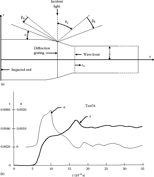
FIGURE 11.11  Diffraction-grating strain gauge method: (a) specimen and (b) testing result. (Courtesy of Dr. Hartman.)

One of the recent applications of this technique is found in a compact microscopic system, which was developed to capture the local strain of a plastic film [14]. A preparatory testing result suggests a high resolution of 442 μm/mm (using a grating of 40–200 lines/mm). Such image processing is also adopted as a sub-pixel technique to define the centroid of the diffracted point with an estimated sensitivity of 0.08 pixel. An example using 80 lines/mm cross grating showed an average strain of 12,000 mm/mm after extension of 0.6 mm by loading.

This technique is not limited to a regularly ruled pattern like a grating, but applicable to any irregular pattern on the surface. One typical system [15] is shown in Figure 11.11, which has a function that automatically checks and evaluates surface quality of a sheet object such as a steel strip and a roll.

11.5    CONCLUSION

In applicative uses of diffraction to the topics described here, one of the problems was detecting a spot or pattern precisely. Although many pioneering studies were reported in the 1970s and 1980s, we had to use detectors such as a photomultiplier, which was a point-wise detector and expensive at that time. Recently, inexpensive CCD cameras have become popular, and, in addition, image and signal processing techniques have made rapid progress. More diffraction-related methods are expected to be explored for metrological applications in industry.

REFERENCES

1.  F. Jenkins and H. White, Fundamentals of Optics, 4th edn., McGraw-Hill, New York, 1976.

2.  K. Iizuka, Engineering Optics, 2nd edn., Springer-Verlag, Berlin, Germany, 1987.

3.  M. Born and E. Wolf, Principles of Optics, 7th edn., Cambridge University Press, Cambridge, U.K., 1999.

4.  E. J. Mittemeijer and P. Scardi (eds.), Diffraction Analysis of the Microstructure of Materials, Springer-Verlag, Berlin, Germany, 2004.

5.  B. Kress and P. Meyrueis, Digital Diffractive Optics: An Introduction to Planar Diffractive Optics and Related Technology, John Willy & Sons, Chichester, U.K., 2000.

6.  J. Goodman, Introduction to Fourier Optics, McGraw-Hill, New York, 1996.

7.  M. Cagnet, M. Francon, and J. C. Thrierr, Atlas of Optical Phenomena, Springer-Verlag, Berlin, Germany, 1962.

8.  M. Cagnet, M. Francon, and J. C. Thrierr, Atlas of Optical Phenomena (Supplement), Springer-Verlag, Berlin, Germany, 1971.

9.  H. Pih and K. C. Liu, Laser diffraction methods for high-temperature strain measurements, Experimental Mechanics 31(3): 60–64, 1991.

10.  T. R. Pryor, O. L. Hageniers, and P. T. North, Diffractographic dimensional measurement, Part 1: Displacement measurement, Applied Optics 11(2): 308–313, 1972.

11.  T. R. Pryor, O. L. Hageniers, and P. T. North, Diffractographic dimensional measurement, Part 2: Profle measurement, Applied Optics 11(2): 314–318, 1972.

12.  A. Ono and T. Komatsu, Ultrasonic vibration analysis by diffractometry, Bulletin of the Japan Society of Precision Engineering 11(2): 101, 102, and 105, 1977.

13.  W. Hartman, Application of the diffraction-grating strain-gage technique for measuring strains and rotations during elastic impact of rods, Experimental Mechanics 14(12): 509–512, 1974.

14.  B. Zhao and A. Asuni, Strain microscope with grating diffraction method, Optical Engineering 38(1): 170–174, 1999.