
CONTENTS
20.2 Optical 3D Measurement Techniques
20.2.4 Laser Speckle Pattern Sectioning
20.3 General Approach to Measure 360° Shape of an Object
20.4 Global and Local Coordinates Translation
20.5 Structured Light Sources, Image Sensors, Camera Model, and Calibration
20.6 Absolute Phase Value Measurement and Discontinuity Ambiguity
20.7 Image Data Patching and CAD Data Comparing
20.8.1 Sensor Planning Examples
20.9.1 Component Shape Measurement
20.9.2 Vehicle Shape Measurement
20.10 Conclusion and Future Research Trend
20.10.2 Direct Shape Measurement from a Specular Surface without Paint
20.10.4 Standard Methodology to Evaluate Optical Shape Measurement System
20.10.5 Large Measurement Range with High Accuracy
20.10.6 Measurement System Calibration and Optimization and Sensor Planning
In industry, there is need for accurately measuring the three-dimensional (3D) shape of objects to expedite and ensure product development and manufacturing quality. There are a variety of applications of 3D shape measurement, such as control for intelligent robots, obstacle detection for vehicle guidance, dimension measurement for die development, stamping panel geometry checking, and accurate stress/strain and vibration measurement. Moreover, automatic online inspection and recognition issues can be converted to the 3D shape measurement of an object under inspection, for example, body panel paint defect and dent inspection. Recently, with the evolution in computer technologies, coupled with the development of digital imaging devices, electro-optical components, laser, and other light sources, 3D shape measurement is now at the point where some techniques have been successfully commercialized and accepted in the industry. For a small-scale depth or shape, micrometer or even nanometer measurements can be reached if a confocal microscope or other 3D microscope is used. However, the key is the relative accuracy or one part out of the measurement depth that poses a real challenge for a large-scale shape measurement. For example, how accurate can a 0.5 m depth measurement be? Moreover, for a large-scale depth and shape measurement, frequently, more cameras and camera positions are required to obtain several shapes from which the final large shape can be patched. It raises the issue of how to patch these shapes together in a highly accurate manner and perform local and global coordinate transforms. This subsequently generates another problem to be solved, namely to overcome lens distortion and aberration. After the 3D shape is obtained, there is a need to compare this data with a computer-generated computer aided engineering (CAE) model.
This chapter is based on the review paper [1] that provides an overview of 3D shape measurement using various optical methods supplemented with some recent developments and updates. Then it focuses on structured light and photogrammetry systems for measuring relatively large-scale and 360° shapes. Various detail aspects such as absolute phase measurement, structured light sources, image acquisition sensors, camera model, and calibration are discussed. Global and local coordinate translation methods, point cloud patching, and computer aided design (CAD) data comparing are also discussed. Several applications are described. Finally, future research trends such as real-time computing, automating, and optimizing sensor placement, and the need for a common standard for evaluation of optical coordinate measurement systems are presented.
20.2 OPTICAL 3D MEASUREMENT TECHNIQUES
Various optical techniques have recently been developed for measuring 3D shape from one position. A comprehensive overview for some of the techniques can be found in the literature [2].
The time-of-flight method for measuring shape is based on the direct measurement of the time of flight of a laser or other light source pulse [3]. During measurement, an object pulse is reflected back to the receiving sensor, and a reference pulse is passed through an optical fiber and received by the sensor. The time difference between the two pulses is converted to distance. A typical resolution for the time-of-flight method is around a millimeter. With sub-picosecond pulses from a diode laser and high-resolution electronics, sub-millimeter resolution is achievable. The recently reported time-correlated single-photon counting method has depth repeatability better than 30 μm at a 1 m standoff distance [4]. Another similar technique is called light-in-flight holography where either short temporal coherence light or very short light pulse is used to generate a motion image of a propagating optical wavefront [5,6]. Combined with digital reconstruction and a Littrow setup, the depth resolution may reach 6.5 μm [7].
Point laser triangulation employs the well-known triangulation relationship in optics. The typical measurement range is ±5 to ±250 mm, accuracy is about one part in 10,000, and frequency is up to 40 kHz or higher [8,9]. A charge-coupled device (CCD) or a position sensitive detector (PSD) is widely used to digitize the point laser image. For PSD, the measurement accuracy is mainly dependent on the accuracy of the image on the PSD. The beam spot reflection and stray light will also affect the measurement accuracy. Masanori Idesawa [10] has developed some methods to improve the accuracy of the PSD by using a high-accuracy kaleidoscopic mirror tunnel position-sensing technique and a hybrid type of PSD. CCD-based sensors avoid the beam spot reflection and stray light effects and provide more accuracy because of the single pixel resolution. Another factor that affects the measurement accuracy is the difference in the surface characteristic of a measured object from the calibration surface. Usually, calibration should be performed on similar surfaces to ensure the measurement accuracy. The recently developed confocal technique can tolerate surface color change, transparency difference, and irregularity without calibration [11].
The Moiré method can be divided into shadow and the more practical projection techniques [12,13]. The key to the Moiré technique is the use of a master grating and a reference grating, from which contour fringes can be generated and resolved by a CCD camera. Increased resolution is realized since the gratings themselves do not need to be resolved by the CCD camera. However, if the reference grating is computer generated as in the logic-Moiré method [14,15], the camera must resolve the master grating. The penalties for the high resolution are the implementation complexity and the need for a high-power light source as compared with a structured light technique. In order to (1) overcome environmental perturbations, (2) increase image acquisition speed, and (3) utilize phase-shift methods to analyze the fringe pattern, snap shot or multiple image Moiré systems have been developed. Two or more Moiré fringe patterns with different phase shifts are simultaneously acquired using multi-camera or image-splitting methods [16,17,18,19,20]. Reference [21] provides a comparison of some high-speed Moiré contouring methods with particular stress on sources of noise and system error functions. The typical measurement range of the phase-shifting Moiré method is from 1 mm to 0.5 m with the resolution at 1/10–1/100 of a fringe. Some novel applications and related references can be found in Refs. [22,23,24,25,26,27,28,29,30,31].
20.2.4 LASER SPECKLE PATTERN SECTIONING
The 3D Fourier transform relationship between optical wavelength (frequency) space and the distance (range) space is used to measure the shape of an object [32,33,34]. Laser speckle pattern sectioning, also known as speckle pattern sampling or laser radar [35,36,37,38], is achieved by utilizing the principle that the optical field in the detection plane corresponds to a two-dimensional (2D) slice of the object’s 3D Fourier transform. The other 2D slices of the object’s 3D transform are acquired by changing the wavelength of the laser. A speckle pattern is measured using a CCD array at each different laser wavelength, and the individual frames are added up to generate a 3D data array. A 3D Fourier transform is applied on this data array to obtain the 3D shape of an object. When a reference plane method [39] is used, this technique is similar to two-wavelength or multiwavelength speckle interferometry. The measurement range can be from a micrometer to a few meters. The accuracy is dependent on the measurement range. With the current laser technology, 1–10 μm resolutions are attained in the measurement range of 10 mm and 0.5 μm measurement uncertainty is achievable (see HoloMapper in the commercial system list). The advantages of this technique are (1) the high flexibility of the measurement range and (2) phase shifting as in conventional interferometry may not be required. The limitation of this technique is that for relatively large-scale shape measurement, it takes more time to acquire the images with the different wavelengths.
The idea behind interferometric shape measurement is that the fringes are formed by variation of the sensitivity matrix that relates the geometric shape of an object to the measured optical phases. The matrix contains three variables; wavelength, refractive index, and illumination and observation directions, from which three methods; two or multiple wavelength [40,41,42,43,44], refractive index change [45,46,47], and illumination direction variation/two sources [48,47,48,49,50,51,52], are derived. The resolution of the two wavelength method depends on the equivalent wavelength (Λ) and the phase resolution of ~Λ/200. For example, two lines of an argon laser (0.5145 and 0.4880 μm) will generate an equivalent wavelength 9.4746 μm and a resolution of 0.09 μm.
Another range measurement technique with high accuracy is double heterodyne interferometry using a frequency shift. Recent research shows it achieves a remarkable 0.1 mm resolution with 100 m range [53]. Interferometric methods have the advantage of being mono-state without the shading problem of triangulation techniques. Combined with phase-shifting analysis, inter-ferometric methods and heterodyne techniques can have an accuracy of 1/100 and 1/1000 of a fringe, respectively. With dedicated optical configuration design, accuracy can reach 1/10,000 of a fringe [54]. The other methods such as shearography [55,56,57], diffraction grating [58,59], digital wave-front reconstruction and wavelength scanning [60,61], and conoscopic holography [62] are also under development. Both shearography and conoscopic holography are collinear systems, which are relatively immune to mechanical disturbances.
Typical photogrammetry employs the stereo technique to measure 3D shapes, although other methods such as defocus, shading, and scaling can also be used. Photogrammetry is mainly used for feature type 3D measurement. It usually needs to have some bright markers such as retroreflective painted dots on the surface of a measured object. In general, photogrammetric 3D reconstruction is established on the bundle adjustment principle in which the geometric model of the central perspective and the orientation of the bundles of light rays in a photogrammetric relationship are developed analytically and implemented by a least square procedure [63]. Extensive research has been done to improve the accuracy of photogrammetry [64,65,66,67,68]. Recent advances make it achieve high accuracy as one part in hundred thousand or even one part in a million [69]. For some fundamental description, one may refer to the website www.geodetic.com/Whatis.htm. There are quite a few of commercially available systems and they may be found by searching the web.
A laser tracker uses an interferometer to measure distances, and two high-accuracy angle encoders to determine vertical and horizontal angles. The laser tracker SMART 310, developed at the National Bureau of Standards, was improved at API (Automated Precision Inc.) to deliver 1 μm range resolution and 0.72 angular resolution [70]. The laser tracker is a scanning system and usually is used to track the positions of optical sensors or robots. The Leica LTD 500 system can provide an absolute distance measurement with accuracy of about ±50 μm and angle encoders that permit accuracy of five parts in a million within a 35 m radius measurement volume [71].
With recent progress in laser tracker technology, the measurement range is increasing. For example, FARO laser tracker Xi has a 230 ft range and accuracy on ADM (absolute distance measurement) can be around 0.001”. The LTD840’s measurement range reaches 262 ft and ADM can be around 0.001” accuracy. API TRACKER 3 renders a 400 ft range and ADM can be around 0.001” accuracy.
The structured light method, also categorized as active triangulation, includes both projected coded light and sinusoidal fringe techniques. Depth information of the object is encoded into a deformed fringe pattern recorded by an image acquisition sensor [72,73,74,75]. Although related to projection Moiré techniques, shape is directly decoded from the deformed fringes recorded from the surface of a diffuse object instead of using a reference grating to create Moiré fringes. One other related technique uses projected random patterns and a trilinear tensor [76,77,78,79]. When a LCD/DMD (liquid crystal projector/digital mirror display) based and optimized shape measurement system is used, the measurement accuracy may be achieved at one part in 20,000 [80]. The structured light method has the following merits: (1) easy implementation, (2) phase shifting, fringe density, and direction change can be realized with no moving parts if a computer-controlled LCD/DMD is used, and (3) fast full-field measurement. Because of these advantages, the coordinate measurement and machine vision industries have started to commercialize the structured light method (see the list) and some encouraging applications can be found in Refs. [81,82,83]. However, to make this method even more accepted in industry some issues have to be addressed, including the shading problem, which is inherent to all triangulation techniques. The 360° multiple-view data registration and defocus with projected gratings or dots promise a solution [84,85,86]. These are discussed briefly in the following sections. For small objects using a microscope, lateral and depth resolutions of 1 and 0.1 μm, respectively, can be achieved [87,88]. Using confocal microscope for shape measurement can be found in Ref. [89].
20.3 GENERAL APPROACH TO MEASURE 360° SHAPE OF AN OBJECT
The global coordinate system is set up and local coordinates systems are registered during measurement. A structured light imaging system is placed at an appropriate position to measure 3D shape from one view, and the absolute phase value at each object point is calculated. These phase values and a geometric-optic model of the measurement system determine the local 3D coordinates of the object points. Three ways are usually used to measure 360° shape, the object rotation method [90,91,92,93,94], the camera/imaging system transport technique, and the fixed imaging system with multiple cameras approach. For camera transport, which is usually for measuring large objects, the measurement is repeated at different views to cover the measured object. All the local 3D coordinates are transformed into the global coordinate system and patched together using a least squares fit method. The measured final 3D coordinates of the object may be compared with CAD master data in a computer using various methods in which the differentiation comparison technique and least square fit are often used.
20.4 GLOBAL AND LOCAL COORDINATES TRANSLATION
For a 360° 3D measurement of an object, an optical sensor has to be positioned at different locations around the object [95,96]. The point clouds obtained at each position need to be input or transformed into global coordinates from each local coordinate so that these point clouds can be patched together to generate the final data set. This can be achieved by multiple cameras at different positions at the same time or a single camera at different position at different time. In order to accomplish this, each sensor coordinate system location and orientation has to be known or measured. Any error in measuring and calculating the sensor location and orientation will cause a propagation error in the global coordinates which will prevent a high over-all accuracy of the final measurement. There are several approaches to determine the relationship between the global and local coordinate systems: (1) accurate mechanical location and orientation of the sensor (local coordinate system), (2) optical tracking of the location and orientation of the sensor using active or passive targets attached to the sensor, and (3) photogrammetry of markers accurately fixed in the object field and hybrid methods. Figure 20.1 shows these approaches. With the recent development in photogrammetry, projected marks can be used [115].
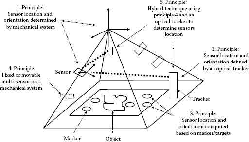
FIGURE 20.1 Sensor planning diagram showing several approaches to determine the relationship between the global and local coordinate systems.
For the mechanical approach 1, the sensor is attached on a mechanical positioning system of high accuracy. The location and orientation of the sensor are derived from the system coordinate and angle information. The advantage of the mechanical system is that it is robust and of high accuracy. However, the cost for accuracy mechanical devices, overcoming environmental perturbation, and maintenance of the equipment is very high.
For the optical approach 2, the local coordinate system is calculated from the measured global position of reference targets (active or passive, with the known local coordinates) on the frame of the optical sensor using an optical tracker system. The advantage is portability and compactness. However, the sensor targets have to be visible and this limits the flexibility. Moreover, floor vibration effect has to be considered. If a high-accuracy tracking system is used, such as laser tracking system, the cost is also relatively high. Both mechanical and optical methods are prone to angular error.
The photogrammetry approach 3 can provide high-accuracy local coordinate system location and orientation from measurement of the global coordinates of makers accurately fixed in the object field. The accuracy can be as high as one part in a million [69]. Conservatively, accuracy can be as one part in 100,000. However, the key limitation for this method is that registration markers have to be placed on or around the object. This increases the measurement time and automation complexity.
20.5 STRUCTURED LIGHT SOURCES, IMAGE SENSORS, CAMERA MODEL, AND CALIBRATION
The light source is important for the overall accuracy of a 3D shape measurement system. Important parameters include uniformity, weight, intensity profile, and speckle/dot size. The projection of a Ronchi grating slide provides high resolution with bright images and is currently used in some commercial systems. However, to calculate absolute distance, multiple grating slides are needed to apply the phase-shift method and to vary the grating frequency. This in turn results in slow speed and relatively large space for storing different gratings. Around 1991–1993, LCDs using incoherent light [97,98,99,100,101,102,103,104] have been used in which each pixel can be addressed by a computer image-generating system. The advantage of this type of projection is the high speed for phase shifting and variable grating frequency. The disadvantage is that LCDs need powerful light sources resulting in cooling concerns and increased weight. Moreover, the resolution is low compared with the film-slide-based light projection. To overcome the brightness concern of the LCD, the reflective LCD, the gas plasma display (GPD), and DMD [105,106,107] have been developed. In addition, the gaps between DMD mirrors are smaller than those pixels between the LCD so that the DMD images are relatively sharper. A detailed error analysis and optimization of a shape measurement system using a LCD/DMD-type fringe projector can be found in Ref. [107]. The LCD, GPD, and DMD have RGB color by which simultaneously acquisition of three images or three phase-shifted images can be used, and this makes the phase-shift technique immune to environmental perturbation [108]. The color advantage may also be used for absolute phase determination [109,108,109,110,111,112,113]. Other light sources are the two point source laser interferometer using a Mach–Zhender configuration [114], fiber optics [115], birefringence crystal [116], acoustic optical modulator [117], and Lasiris’ non-Gaussian-structured light projector using a specially designed prism that can generate 99 lines with inter-beam angle at 0.149° [118].
In optical 3D shape measurement, image acquisition is a key factor for accuracy. Currently, images are acquired using a CCD or a charge injection device (CID) sensor. There are full frame, frame transfer, and interline transfer sensors. The major concerns regarding these sensors are the speed, resolution, dynamic range, and accuracy. Up to 5k × 5k pixel CCD sensors are commercially available such as DALSA IA-D9-5120, Ford Aerospace 4k × 4k, Kodak Model 16.8I (4k × 4k), and Loral CCD481, to name a few. Usually, the high-resolution sensor is a full-frame CCD that does not have storage and needs to have a shutter to allow image transfer that results in relatively slow speed. Combined with micro- and macro-scanning techniques, the image resolution can be 20k × 20k, which is equivalent to the resolution of a 20 cm × 20 cm area photographic film with 100 lines/mm. The CID sensor differs from a CCD sensor in that it does not bloom though overexposure and can be read out selectively since each pixel is individually addressed.
A high-accuracy CCD sensor or a video camera requires high radiometric and geometric accuracy, including both intrinsic parameters, such as lens distortion, and extrinsic parameters, such as the coordinate location and orientation of the camera. A detailed discussion regarding characterization and calibration of radiometric and geometric feature of a CCD sensor can be found in Ref. [119]. The relative accuracy of one part in 1000 can be achieved using on-site automatic calibration during measurement. More accurate calibration, such as 10−4 to 10−5 accuracy, may be achieved using a formal off-line calibration procedure with a more complex and nonlinear camera model. A high-accuracy camera model is necessary to characterize the lens aberration and to correct the captured image for the distortions caused by the aberration [120,121,122,123,124,125,126,127,128]. The calibration of an optical measurement system can be further divided into a geometric parameter technique as described above and geometric transformation approach. The geometric parameter technique requires the known parameters of the optical setup including the projector and the image sensor. On the other hand, it is not essential to know the parameters of the image system in the geometric transformation approach [129,130,131,132,133,134], in which the recently developed projection or image ray tracing technique is discussed [132] and the known position of the object or camera variation approach is provided [133]. Once the imaging system is moved or the measured object size/depth is changed, the calibration procedure may be performed again. This, however, may pose some limitation for this method. Reference [135] developed a self-calibration approach that may reduce the complexity of calibration procedure and increase accuracy.
20.6 ABSOLUTE PHASE VALUE MEASUREMENT AND DISCONTINUITY AMBIGUITY
In general, using phase-shifted structured light to measure the 3D shape of the object only renders relative phase values. Phase shifting determines the fractional order of fringes at any pixel. These fractional orders are connected together using their adjacent integer orders, which is called unwrapping process. However, when the phase difference between the adjacent pixels is larger than 2π, such as occurs at a discontinuity or steep change of shape, the integer fringe order becomes ambiguous. Recently, several methods have been developed to overcome discontinuities [75,136,135,136,137,138,139,140,141,142,143,144,145,146,147,148,149,150,151,152,153,154,155,156,157,158,159]. The basic idea is that changing the measurement system’s sensitivity results in fringe or projected structured strip density changes. This means that the integer order of the fringes sweep through the discontinuity. It can be viewed both in spatial and temporal domains, and results in various methods. As mentioned in Ref. [144], the key to overcoming discontinuity is to determine the fringe order n during unwrapping process. These methods, such as two wavelength or parameter change, are used in interferometry to determine absolute fringe fractional and integer orders [160,161,162,163,164]. In plane, rotation of the grating and varying the grating frequency (e.g., fringe projection with two point variable spacing) are useful techniques. Triangulation and stereography can also be employed to determine absolute phase values and overcome discontinuity, although there are limitations since all pixel points may not be covered without changing setup. Some direct phase calculation, such as phase derivative methods without phase unwrapping, may still need continuous condition [165]. However, the same problem can also be solved by phase-locked loop technique [166].
20.7 IMAGE DATA PATCHING AND CAD DATA COMPARING
After processing the 360° local images, the local point cloud patches need to be merged together to obtain a final global point cloud of the object. The accuracy of a measurement system is also determined by the matching accuracy. There is extensive research on the matching methods and algorithms in photogrammetry, which can generally be categorized as area-based matching, feature-based matching, and other methods such as centroid method [167,168,169,170,171,172]. The area-based matching takes advantage of correlation coefficient maximization and least squares minimization, while feature-based matching exploits all algorithms extracting features of points, lines, and areas. Area-based matching usually employs pixel intensity as constraint, while feature-based matching uses geometric constraint. All the above methods require sub-pixel accuracy to achieve overall accuracy. Under optimized condition, 0.02 pixel accuracy can be achieved [173,174,175] and in general 0.05 pixel accuracy should be obtained [175]. There is a discussion between sub-pixel accuracy and geometric accuracy where geometric accuracy is more promising [176].
For CAD data comparison, the differentiation and least mean square methods are mainly used. The measured point cloud data are subtracted from CAD data to obtain differences as an error indicator. The comparison to the appropriate CAD model can be used to obtain the best fit of registration between the two. Model matching can start with a selection of a subset of point cloud data. The measured point data in this subset are matched to the CAD data by making the normal vector collinear to the normal vector of the local CAD surface. The distances in the normal direction between the CAD surface and measured point cloud are fed into a least square error function. The best fit is achieved by optimizing the least square error function [95,96,177]. Before the measured data can be compared to CAD master data, it needs to be converted into standard CAD representations [178,179,180]. This is usually done by first splitting the measured data into major geometric entities and modeling these entities in the nonuniform rational B-spline surface form; this has the advantage of describing the quadric in addition to free-form surface using a common mathematical solution.
Large-scale surface inspection often requires either multiple stationary sensors or relocation of a single sensor for obtaining the 3D data. A multi-sensor system has an advantage on high-volume inspection of similar products, but usually lacks flexibility. In order to improve the flexibility, various portable sensor systems and automated eye-on-hand systems are produced. However, no matter what kinds of sensor systems be used, the first and most critical problem that should be solved is how the sensors can be placed to successfully view the 3D object without missing required information. Given the information about the environment (e.g., the observed objects and the available sensors) and information about the mission (i.e., detection of certain object features, object recognition, scene reconstruction, object manipulation, and accurate, dense enough point clouds), strategies should be developed to determine sensor parameters that achieve the mission with a certain degree of satisfaction. Generally, solving such a problem is categorized as a sensor planning problem. Considerable effort on general techniques has been made in sensor planning. We can collect them into the following four categories.
1. Generate-and-test approach [181,182,183]: By using this method, sensor configurations are generated first, then evaluated using performance functions and mission constraints. In order to avoid an exhausting search process, the domain of sensor configurations is discretized by tessellating a viewing sphere surrounding the object under observation. This is a time-consuming technique without guaranteeing an optimal result.
2. Synthesis approach [184,185,186,187,188,189,190]: This approach is built upon an analytical relation between mission constraints and sensor parameters. It has a beautiful and promising theoretical framework that can determine the sensor configurations for certain cases. The drawback of this approach is that the analytical relations sometimes are missing, especially when constraints are complex.
3. Sensor simulation system [191,192,193]: This system brings objects, sensors, and light sources into a unified virtual environment. It then uses the generate-and-test approach to find desired sensor configurations. The simulation systems are useful in the sense that operators can actively evolve the process and ensure the results.
4. Expert system approach [194,195,196,197]: Rule-based expert systems are utilized to bridge reality and expert knowledge of viewing and illumination. The recommended sensor configurations are the output of the expert system from reality checking. In general, the more complete knowledge we have, the “wiser” the advice we can get.
20.8.1 SENSOR PLANNING EXAMPLES
In fact, these sensor-planning techniques have strong application background. Their goal is aggressively set to improve machine intelligence and reduce human-intensive operations that cause the long development cycle time, high cost, and complexity in modern industry. Several examples are (1) an intelligent sensor-planning system was conceptually defined to be applied in the application of automated dimensional measurements by using CAD models of measured parts [198], (2) an inspection system is able to determine appropriate and flexible action in new situations since online sensor-planning techniques were adopted [199], and (3) the techniques were applied to a robot vision system so that the orientation and position of vision sensors and a light source can be automatically determined [200].
20.9.1 COMPONENT SHAPE MEASUREMENT
During component development cycle, there is a tryout phase that requires measurement of the shape of a component or the die to make the component. The following is a demonstration of using a 3D optical measurement setup to measure a component and compare it to the master CAD data to evaluate the spring back effect. Figure 20.2 shows the point cloud data of a component. Figure 20.3 shows the corresponding CAD data. Figure 20.4 shows the comparison between the measured data and CAD data, in which the two sets of data are compared using the least square fit.
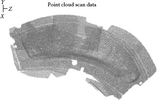
FIGURE 20.2 Measured point cloud data of a component.
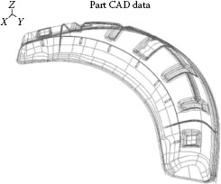
FIGURE 20.3 Corresponding CAD data of a component.
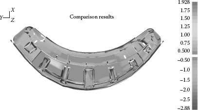
FIGURE 20.4 Comparison between the measured data and CAD data of a component.
20.9.2 VEHICLE SHAPE MEASUREMENT
For rapid prototyping or benchmarking, often the vehicle body shape needs to be measured. The following example uses the structured light method combined with photogrammetry to measure car body shape. Some coded targets were placed on the vehicle body to permit local to global coordinate transformation. Then structured light was projected on the vehicle surface combined with phase shifting and absolute phase measurement technique using fringe frequency change to determine the local coordinate pixel by pixel at one view direction. The 240 view directions were used to cover the whole vehicle surface (it is a real vehicle). Then the 240 point clouds were patched together using a least mean square method. The point cloud data were extracted using 1 out of 8 pixels. The shaded measured data is shown in Figure 20.5 and the point cloud data is shown in Figure 20.6.
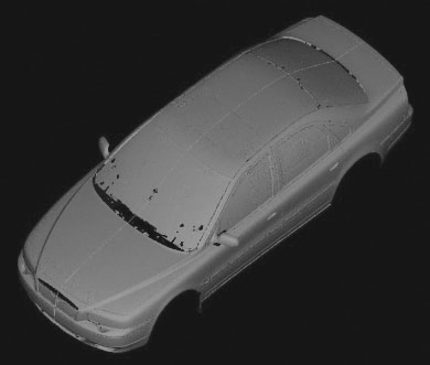
FIGURE 20.5 Shaded measured data of a vehicle.
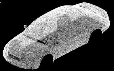
FIGURE 20.6 Measured point cloud data of a vehicle.
For accurate analysis of vibration or strain, the geometric information of the tested structure needs to be known. Using the two-wavelength shape measurement method, the vibration amplitude, phase, and geometric information of a tested structure can be measured using a single compact Electronic Speckle Pattern Inter ferometry (ESPI) setup [201]. Figure 20.7a and b shows the four vibration states of a corrugated plate clamped along its boundaries and subjected to harmonic excitation at 550 Hz. The state 1 in Figure 20.7a depicts the original corrugated plate geometric shape and the rest are vibrating states at distinct times. From Figure 20.7 one can clearly see the shape effect on vibration.
The geometry measurement technique can also be applied to measure paint defects of a body panel of a vehicle, although it is a challenge to detect small flaws in large areas. A methodology has been developed as shown in the flow chart in Figure 20.8, in which structured light generated from a monitor is reflected from the tested panel and digitized into a computer image processing system. Then the digital Fourier transform method is used to extract the global shape of the panel by selecting the structured light frequency. The defect geometry coupled with the global shape of the panel is calculated by selecting half-spatial frequencies. The defect geometry is finally obtained by subtracting the above two results as shown in Figure 20.9, where Figure 20.9a shows the panel with projected structured light and Figure 20.9b shows the final measurement result. One can see that without the calculation, one can only observe the large defects by enhanced fringe modulation. Figure 20.10 shows the optical setup. The measurement area is about 0.25 m × 0.25 m and the minimum defect size is about 250 μm [202]. Some other application examples can be found in Refs. [203,204], to name a few.
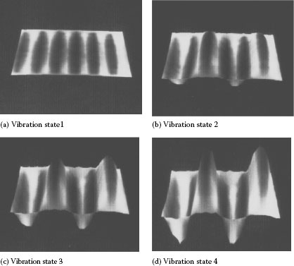
FIGURE 20.7 (a) Vibration state 1 depicts the original corrugated plate geometric shape and (b–d) vibration states 2–4 show the effect of the underlying shape.
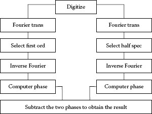
FIGURE 20.8 Structured light generated from a monitor and reflected from the test panel and digitized into a computer image processing system.
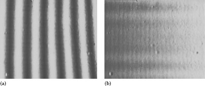
FIGURE 20.9 (a) Panel with projected structured light and (b) defects in the final measurement result.
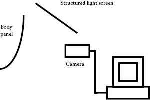
FIGURE 20.10 Optical setup showing structured light generated from a monitor reflected from the panel and digitized into a computer image processing system.
20.10 CONCLUSION AND FUTURE RESEARCH TREND
The principles of triangulation, structured light, and interferometry have been in existence for decades. However, it is only with the recent availability of advanced and low-cost computers, electro-optical elements, and lasers that such techniques have reached the breakthrough point to be commercialized, and are increasingly being applied in industry. To make it even more acceptable in industry and to strive to achieve 10−4 to 10−5 accuracy [80,135], there are still some challenges that need to be addressed. The following may provide some future trends. Table 20.1 shows some full-field shape measurement commercial systems based on leading edge technologies.
TABLE 20.1
Some Full Field Shape Measurement Commercial Systems Based on Leading Edge Technologies
System |
Principle |
Accuracy on Volume |
Atos System: Capture 3D, Costa Mesa, CA 92626, Tel.: 1-714-546-7278 |
Structured light + photogrammetry, 360° view/patching |
About 50 μm (2σ) on relatively large volume |
Comet/OptoTrak System: 4000 Grand River Ave., [email protected] |
Structured light + optical tracking, 360° view/patching |
About 50 μm (2σ) on relatively large volume |
Optigo/CogniTens System: US, Tel.: 1-815-637-1926 |
Random dot pattern + photogrammetry + view/patching |
About 20–100 μm (2σ) on medium volume |
4DI System: IA, 149 Sidney St., Cambridge, MA 02139, Tel.: 1-617-354-3830 |
Structured light + real time computing, one view/no patching |
About 10–3 on medium volume |
HoloMapper System: ERIM International, Inc. 1975 Green Rd., Ann Arbor, MI 48105, Tel.: 1-313-994-0287 |
Laser radar/multiple wavelength, one view/no patching |
Uncertainty 0.5 μm on medium volume |
Real-time 3D shape measurement is an ongoing request in industry to drive down product cost and increase productivity and quality. The major impact will be in digital design, digital and physical manufacturing, and fast prototyping that streamline and integrate product design and manufacture. Real-time 3D shape measurement is the key for successfully implementing 3D coordinate display and measurement, manufacturing control, and online quality inspection. An encouraging example of this is jigless assembly based on the real-time, simultaneous measurement of different but related components. Described by Hobrough [205], real time is to assign a Z-value or depth for every pixel within a 17 ms cycle, which corresponds to the integration time of a CCD sensor. Recently, over 100 measured points for every 40 ms was achieved using photogrammetry [206], and there is a report on the real-time 3D shape measurement system [207]. The key for real time is a high computational speed that can meet online manufacturing needs.
20.10.2 DIRECT SHAPE MEASUREMENT FROM A SPECULAR SURFACE WITHOUT PAINT
There is an urgent need, but little research activity, in the area of using optical techniques to measure the 3D shape of an object with specular surface, such as a die surface. There are some efforts to develop techniques in this area. References [208,209] proposed a technique using four lights to measure specular features. Reference [210] employed a simplified version of the Torrance–Sparrow reflectance model to retrieve object curvature; this method relied on prior knowledge of surface reflectance. References [211,212] suggested using multiple (127) point sources to detect specular shape. Reference [213] developed a photometry sampling technique employing a matrix of extended sources to determine the specular shape. References [214,215,216,217,218] used diffusive TV screen as structured light source; however, since the diffusive screen has to be placed close to the measurement surface, the illuminated area is limited. References [216,217,218] proposed a retroreflective screen coupled with projection of structured light by which a large area may be visualized. However, the retro-reflective screen has to be rigid, controlled, or calibrated without deformation or movement during the measurement. References [219,220] developed a coaxial linear distance sensor for measuring specular shape of a die surface; however, it is based on point scanning which is not fast enough for the industrial application of measuring large die surface. The current technique for measuring die surfaces requires painting the surface with powder, which slows measurement speed and reduces measurement accuracy.
There is a lack of research activity for overcoming shading problem inherent in triangulation methods, although some other methods [84,85,86] besides interferometric and laser speckle sectioning show some progress. These methods use a defocus technique similar to the confocal microscope principle and the newly developed diffraction grating technique [58,59].
20.10.4 STANDARD METHODOLOGY TO EVALUATE OPTICAL SHAPE MEASUREMENT SYSTEM
An international standard needs to be established to evaluate optical shape measurement systems. Important parts of this standard should include the following: (1) standard sample parts with known dimensions, surface finishes, and materials, (2) math assumptions and error characterization, (3) measurement speed and volume capability, (4) repeatability and reproducibility procedures, (5) calibration procedures, and (6) reliability evaluation.
Standard specification/terminology (Table 20.2) is needed to define precision/repeatability and accuracy. An example is, what should be used: accuracy, error, or uncertainty [221]. Many coordinate measurement manufacturers specify a range accuracy of ±x μm. Some manufacturers try to specify measurement accuracy as 1σ, 2σ, or 3σ. The ISO/R 1938–1971 standard employs a 2σ band [222].
Accuracy |
The closeness of the agreement between the result of a measurement and the value of the quantity subject to measurement, that is, the measurand [221]. |
Uncertainty |
The estimated possible deviation of the result of measurement from its actual value [224]. |
Error |
The result of a measurement minus the measured value [221]. |
Precision |
The closeness of agreement between independent test results obtained under stipulated conditions [221]. |
Repeatability |
The closeness of the agreement between the results of successive measurements of the same measurand carried out under the same conditions of measurement [221]. |
Reproducibility |
The closeness of the agreement between the results of measurements of the same measurand carried out under changed conditions of measurement [221]. |
Resolution |
A measure of the smallest portion of the signal that can be observed [224]. |
Sensitivity |
The smallest detectable change in a measurement. The ultimate sensitivity of a measuring instrument depends both on its resolution and the lowest measurement range [224]. |
20.10.5 LARGE MEASUREMENT RANGE WITH HIGH ACCURACY
Most shape measuring systems trade off measurement accuracy for measurement range. However, there is an industrial need for systems that have a large measurement range and high accuracy. Further research needs to be done in this area, though there is encouraging report in which the shape of a 4 m wide area of a brick wall was measured using fringe projection [223].
20.10.6 MEASUREMENT SYSTEM CALIBRATION AND OPTIMIZATION AND SENSOR PLANNING
System calibration and optimization are key factors to stretch the measurement accuracy [80] and to achieve 10−4 to 10−5 accuracy [135]. Reference [80] shows how to use the same system but with optimization to achieve one order higher accuracy and Ref. [135] demonstrates how to use the novel self-calibration to accomplish mathematically estimated approximately 10−5 accuracy. Sensor planning will help to fulfill the above goals. Reference [135] also provides a way to eliminate markers using photogrammetry that is one step further to make 3D optical methods be more practical in industry.
The authors thank T. Cook, B. Bowman, C. Xi, E. Liasi, P. Harwood, and J. Rankin for providing test setup, data registration and processing, and test results, and T. Allen for his valuable suggestions.
1. F. Chen, G. M. Brown, and M. Song, Overview of three-dimensional shape measurement using optical methods, Opt. Eng., 39(1), 10–22, 2000.
2. H. J. Tiziani, Optical metrology of engineering surfaces—Scope and trends, in Optical Measurement Techniques and Applications, P. K. Rastogi (Ed.), Artech House Inc., London, U.K., 1997.
3. I. Moring, H. Ailisto, V. Koivunen, and R. Myllyla, Active 3-D vision system for automatic model-based shape inspection, Opt. Lasers Eng., 10(3 and 4), 1989.
4. J. S. Massa, G. S. Buller, A. C. Walker, S. Cova, M. Umasuthan, and A. Wallace, Time of flight optical ranging system based on time correlated single photon counting, Appl. Opt., 37(31), 7298–7304, 1998.
5. N. Abramson, Time reconstruction in light-in-flight recording by holography, Appl. Opt., 30, 1242–1252, 1991.
6. T. E. Carlsson, Measurement of three dimensional shapes using light-in-flight recording by holography, Opt., Eng., 32, 2587–2592, 1993.
7. B. Nilsson and T. E. Carlsson, Direct three dimensional shape measurement by digital light-in-flight holography, Appl. Opt., 37(34), 7954–7959, 1998.
8. Z. Ji and M. C. Leu, Design of optical triangulation devices, Opt. Laser Technol., 21(5), 335–338, 1989.
9. C. P. Keferstein and M. Marxer, Testing bench for laser triangulation sensors, Sensor Rev., 18(3), 183–187, 1998.
10. M. Idesawa, High-precision image position sensing methods suitable for 3-D measurement, Opt. Lasers Eng., 10(3 and 4), 1989.
11. Keyence technical report on sensors & measuring instruments, 1997.
12. H. Takasaki, Moiré topography, Appl. Opt., 9, 1467–1472, 1970.
13. K. Harding and R. Tait, Moiré techniques applied to automated inspection of machined parts, SME Vision’86 Conference, Detroit, MI, 1986.
14. A. Asundi, Computer aided Moiré methods, Opt. Lasers Eng., 17, 107–116, 1993.
15. C. M. Wong, Image processing in experimental mechanics, MPhil thesis, the University of Hong Kong, Pokfulam, Hong Kong, 1993.
16. Y. Arai, H. Hirai, and S. Yokozeki, High-resolution dynamic measurement using electronic speckle pattern interferometry based on multi-camera technology, Opt. Lasers Eng., 46(10), 733–738, 2008.
17. A. J. P. van Haasteren and H. J. Frankena, Real time displacement measurement using a multicamera phase stepping speckle interferometer, Appl. Opt., 33(19), 4137–4142, 1994.
18. M. Kujawinska, L. Salbut, and K. Patorski, Three channels phase stepped system for Moiré interferometry, Appl. Opt., 30(13), 1991.
19. F. Chen, Y. Y. Hung, and J. Gu, Dual fringe pattern phase shifting interferometry for time dependent phase evaluation, SEM Proceedings on VII International Congress on Experimental Mechanics, 1992.
20. L. Bieman and K. Harding, 3D imaging using a unique refractive optic design to combine Moiré and stereo, Proc. SPIE, 3206, 1997.
21. K. Harding, High speed Moiré contouring methods analysis, Proc. SPIE, 3520, 27, 1998.
22. J. J. Dirckx and W. F. Decraemer, Video Moiré topography for in-vitro studies of the eardrum, Proc. SPIE, 3196, 2–11, 1998.
23. K. Yuen, I. Inokuchi, M. Maeta, S. Manabu, and Y. Masuda, Dynamic evaluation of facial palsy by Moiré topography video: Second report, Proc. SPIE, 2927, 138–141, 1996.
24. Y.-B. Choi and S.-W. Kim, Phase shifting grating projection Moiré topography, Opt. Eng., 37(3), 1005–1010, 1998.
25. T. Matsumoto, Y. Kitagawa, and T. Minemoto, Sensitivity variable Moiré topography with a phase shift method, Opt. Eng., 35(6), 1754–1760, 1996.
26. T. Yoshizawa and T. Tomisawa, Shadow Moiré topography by means of the phase shift method, Opt. Eng., 32(7), 1668–1674, 1993.
27. T. Yoshizawa and T. Tomisawa, Moiré topography with the aid of phase shift method, Proc. SPIE, 1554B, 441–450, 1991.
28. J. F. Cardenas-Garcia, S. Zheng, and F. Z. Shen, Projection Moiré as a tool for the automated determination of surface topography, Proc. SPIE, 1554B, 210–224, 1991.
29. T. Matsumoto, Y. Kitagawa, M. Adachi, and A. Hayashi, Laser Moiré topography for 3D contour measurement, Proc. SPIE, 1332, 530–536, 1991.
30. J. E. A. Liao and A. S. Voloshin, Surface topography through the digital enhancement of the shadow Moiré, SEM Proceedings, pp. 506–510, 1990.
31. J. S. Lim and M. S. Chung, Moiré topography with color gratings, Appl. Opt., 27, 2649, 1988.
32. J. Y. Wang, Imaging laser radar—An over view, Proceedings of the Ninth International Conference Laser’86, pp. 19–29, 1986.
33. J. C. Marron and K. S. Schroeder, Three dimensional lensless imaging using laser frequency diversity, Appl. Opt., 31(2), 255–262, 1992.
34. J. C. Marron and T. J. Schulz, Three dimensional, fine resolution imaging using laser frequency diversity, Opt. Lett., 17, 285–287, 1992.
35. L. G. Shirley, Speckle decorrelation techniques for remote sensing of rough object, OSA Annu. Meet. Tech. Dig., 18, 208, 1989.
36. L. G. Shirley, Remote sensing of object shape using a wavelength scanning laser radar, OSA Annu. Meet. Tech. Dig., 17, 154, 1991.
37. G. R. Hallerman and L. G. Shirley, A comparison of surface contour measurements based on speckle pattern sampling and coordinate measurement machines, Proc. SPIE, 2909, 8997, 1996.
38. T. Dressel, G. Häusler, and H. Venzhe, Three dimensional sensing of rough surfaces by coherence radar, Appl. Opt., 31, 919–925, 1992.
39. L. G. Shirley and G. R. Hallerman, Application of tunable lasers to laser radar and 3D imaging, Technical Report No. 1025, MIT Lincoln Laboratory, Lexington, MA, 1996.
40. K. A. Haines and B. P. Hildebrand, Contour generation by wavefront construction, Phys. Lett., 19, 10–11, 1965.
41. K. Creath, Y. Y. Cheng, and J. Wyant, Contouring aspheric surface using two-wavelength phase shifting interferometry, Opt. Acta, 32(12), 1455–1464, 1985.
42. R. P. Tatam, J. C. Davies, C. H. Buckberry, and J. D. C. Jones, Holographic surface contouring using wavelength modulation of laser diodes, Opt. Laser Technol., 22, 317–321, 1990.
43. T. Maack, G. Notni, and W. Schreiber, Three coordinate measurement of an object surface with a combined two-wavelength and two-source phase shifting speckle interferometer, Opt. Commun., 115, 576–584, 1995.
44. Y. Yu, T. Kondo, T. Ohyama, T. Honda, and J. Tsujiuchi, Measuring gear tooth surface error by fringe scanning interferometry, Acta Metrologica Sin., 9(2), 120–123, 1986.
45. J. S. Zelenka and J. R. Varner, Multiple-index holographic contouring, Appl. Opt., 8, 1431–1434, 1969.
46. Y. Y. Hung, J. L. Turner, M. Tafralian, J. D. Hovanesian, and C. E. Taylor, Optical method for measuring contour slopes of an object, Appl. Opt., 17(1), 128–131, 1978.
47. H. Ei-Ghandoor, Tomographic investigation of the refractive index profiling using speckle photography technique, Opt. Commun., 133, 33–38, 1997.
48. N. Abramson, Holographic contouring by translation, Appl. Opt., 15, 1018–1022, 1976.
49. C. Joenathan, B. Franze, P. Haible, and H. J. Tiziani, Contouring by electronic speckle pattern interferometry using dual beam illumination, Appl. Opt., 29, 1905–1911, 1990.
50. P. K. Rastogi and L. Pflug, A holographic technique featuring broad range sensitivity to contour diffuse objects, J. Mod. Opt., 38, 1673–1683, 1991.
51. R. Rodrfguez-Vera, D. Kerr, and F. Mendoza-Santoyo, Electronic speckle contouring, J. Opt. Soc. Am. A, 9(1), 2000–2008, 1992.
52. L. S. Wang and S. Krishnaswamy, Shape measurement using additive-subtractive phase shifting speckle interferometry, Meas. Sci. Technol., 7, 1748–1754, 1996.
53. E. Dalhoff, E. Fischer, S. Kreuz, and H. J. Tiziani, Double heterodyne interferometry for high precision distance measurements, Proc. SPIE, 2252, 379–385, 1993.
54. J. D. Trolinger, Ultrahigh resolution interferometry, Proc. SPIE, 2861, 114–123, 1996.
55. J. R. Huang and R. P. Tatam, Optoelectronic shearography: Two wavelength slope measurement, Proc. SPIE, 2544, 300–308, 1995.
56. C. T. Griffen, Y. Y. Hung, and F. Chen, Three dimensional shape measurement using digital shearography, Proc. SPIE, 2545, 214–220, 1995.
57. C. J. Tay, H. M. Shang, A. N. Poo, and M. Luo, On the determination of slope by shearography, Opt. Lasers Eng., 20, 207–217, 1994.
58. T. D. DeWitt and D. A. Lyon, Range-finding method using diffraction gratings, Appl. Opt., 23(21), 2510–2521, 1995.
59. T. D. Dewitt and D. A. Lyon, Moly: A prototype hand-held 3D digitizer with diffraction optics, Opt. Eng., 39, 2000.
60. S. Seebacher, W. Osten, and W. Jüptner, Measuring shape and deformation of small objects using digital holography, Proc. SPIE, 3479, 104–115, 1998.
61. C. Wagner, W. Osten, and S. Seebacher, Direct shape measurement by digital wave-front reconstruction and wavelength scanning, Opt. Eng., 39(1), 2000.
62. G. Sirat and F. Paz, Conoscopic probes are set to transform industrial metrology, Sensor Rev., 18(2), 108–110, 1998.
63. W. Wester-Ebbinghaus, Analytics in non-topographic photogrammetry, ISPRS Congress, Commission V, Kyoto, Japan, Vol. 27, Part B11, pp. 380–390, 1988.
64. H. M. Karara, Non-Topographic Photogrammetry, 2nd edn., American Society of Photogrammetry and Remote Sensing, Falls Church, VA, 1989.
65. A. Gruen and H. Kahmen (Eds.), Optical 3-D Measurement Techniques, Wichmann, Heidelberg, Germany, 1989.
66. A. Gruen and H. Kahmen (Eds.), Optical 3-D Measurement Techniques II, SPIE Vol. 2252, 1993.
67. A. Gruen and H. Kahmen (Eds.), Optical 3-D Measurement Techniques III, Wichmann, Heidelberg, Germany, 1995.
68. C. C. Slama, Manual of Photogrammetry, 4th edn., American Society of Photogrammetry, Falls Church, VA, 1980.
69. C. S. Fraser, Photogrammetric measurement to one part in a million, Photogrammetric Eng. Remote Sens., 58(3), 305–310, 1992.
70. W. Schertenleib, Measurement of structures (surfaces) utilizing the SMART 310 laser tracking system, Optical 3-D Measurement Techniques III, Wichmann, Heidelberg, Germany, 1995.
71. S. Kyle, R. Loser, and D. Warren, Automated Part Positioning with the Laser Tracker, Eureka Transfers Technology, 1997.
72. V. Sirnivasan, H. C. Liu, and M. Halioua, Automated phase measuring profilometry of 3D diffuse objects, Appl. Opt., 23, 3105–3108, 1984.
73. J. A. Jalkio, R. C. Kim, and S. K. Case, Three dimensional inspection using multi-stripe structured light, Opt. Eng., 24(6), 966–974, 1985.
74. F. Wahl, A coded light approach for depth map acquisition, in Mustererkennung 86, Informatik Fachberichte 125, Springer-Verlag, Berlin, Germany, 1986.
75. S. Toyooka and Y. Iwasa, Automatic profilometry of 3D diffuse objects by spatial phase detection, Appl. Opt., 25, 1630–1633, 1986.
76. M. Sjodahl and P. Synnergren, Measurement of shape by using projected random patterns and temporal digital speckle photography, Appl. Opt., 38(10), 1990–1997, 1999.
77. A. Shashua, Trilinear tensor: The fundamental construct of multiple-view geometry and its applications, International Workshop on Algebraic Frames for the Perception Action Cycle, Kiel, Germany, September 1997.
78. S. Avidan and A. Shashua, Novel view synthesis by cascading trilinear tensors, IEEE Trans. Vis. Comput. Graph., 4(4), 1998.
79. A. Shashua and M. Werman, On the trilinear tensor of three perspective views and its underlying geometry, Proceedings of the International Conference on Computer Vision, Boston, MA, June 1995.
80. C. R. Coggrave and J. M. Huntley, Optimization of a shape measurement system based on spatial light modulators, Opt. Eng., 39(1), 2000.
81. H. Gartner, P. Lehle, and H. J. Tiziani, New, high efficient, binary codes for structured light methods, Proc. SPIE, 2599, 4–13, 1995.
82. E. Muller, Fast three dimensional form measurement system, Opt. Eng., 34(9), 2754–2756, 1995.
83. G. Sansoni, S. Corini, S. Lazzari, R. Rodella, and F. Docchio, Three dimensional imaging based on gray-code light projection: Characterization of the measuring algorithm and development of a measuring system for industrial application, Appl. Opt., 36, 4463–4472, 1997.
84. K. Engelhardt and G. Häusler, Acquisition of 3D data by focus sensing, Appl. Opt., 27, 4684, 1988.
85. A. Serrano-Heredia, C. M. Hinojosa, J. G. Ibarra, and V. Arrizon, Recovery of three dimensional shapes by using a defocus structured light system, Proc. SPIE, 3520, 80–83, 1998.
86. M. Takata, T. Aoki, Y. Miyamoto, H. Tanaka, R. Gu, and Z. Zhang, Absolute three dimensional shape measurements using a co-axial optical system with a co-image plan for projection and observation, Opt. Eng., 39(1), 2000.
87. H. J. Tiziani, Optical techniques for shape measurements, Proceedings of the Second International Workshop on Automatic Processing of Fringe Patterns, Fringe ’93, W. Jüptner and W. Osten (Eds.), Akademie Verlag, Berlin, Germany, 1993.
88. K. Leonhardt, U. Droste, and H. J. Tiziani, Mircoshape and rough surface analysis by fringe projection, Appl. Opt., 33, 7477–7488, 1994.
89. H. J. Tiziani and H. M. Uhde, Three dimensional image sensing with chromatic confocal microscopy, Appl. Opt., 33, 1838–1843, 1994.
90. M. Halioua, R. S. Krishnamurthy, H. C. Liu, and F. P. Chiang, Automated 360° profilometry of 3-D diffuse objects, Appl. Opt., 24, 2193–2196, 1985.
91. X. X. Cheng, X. Y. Su, and L. R. Guo, Automated measurement method for 360° profilometry of diffuse objects, Appl. Opt., 30, 1274–1278, 1991.
92. H. Ohara, H. Konno, M. Sasaki, M. Suzuki, and K. Murata, Automated 360° profilometry of a three-dimensional diffuse object and its reconstruction by use of the shading model, Appl. Opt., 35, 4476–4480, 1996.
93. A. Asundi, C. S. Chan, and M. R. Sajan, 360° profilometry: New techniques for display and acquisition, Opt. Eng., 33, 2760–2769, 1994.
94. A. Asundi and W. Zhou, Mapping algorithm for 360-deg profilometry with time delayed and integration imaging, Opt. Eng., 38, 339–344, 1999.
95. C. Reich, Photogrammetric matching of point clouds for 3D measurement of complex objects, Proc. SPIE, 3520, 100–110, 1998.
96. R. W. Malz, High dynamic codes, self calibration and autonomous 3D sensor orientation: Three steps towards fast optical reverse engineering without mechanical CMMs, Optical 3-D Measurement Techniques III, Wichmann Verlag, Heidelberg, pp. 194–202, 1995.
97. H. J. Tiziani, High precision surface topography measurement, in Optical 3-D Measurement Techniques III, A. Gruen and H. Kahmen (Eds.), Wichmann Verlag, Heidelberg, Germany, 1995.
98. S. Kakunai, T. Sakamoto, and K. Iwata, Profile measurement by an active light source, Proceedings of the Far East Conference on Nondestructive Testing and the Republic of China’s Society for Nondestructive Testing Ninth Annual Conference, pp. 237–242, 1994.
99. Y. Arai, S. Yekozeki, and T. Yamada, 3-D automatic precision measurement system by liquid crystal plate on moire-topography, Proc. SPIE, 1554B, 266–274, 1991.
100. G. Sansoni, F. Docchio, U. Minoni, and C. Bussolati, Development and characterization of a liquid crystal projection unit for adaptive structured Illumination, Proc. SPIE, 1614, 78–86, 1991.
101. A. Asundi, Novel grating methods for optical inspection, Proc. SPIE, 1554B, 708–715, 1991.
102. Y. Y. Hung and F. Chen, Shape measurement using shadow Moiré with a teaching LCD, Technical Report, Oakland University, Rochester, MI, 1991.
103. Y. Y. Hung and F. Chen, Shape measurement by phase shift structured light method with a LCD, Technical Report, Oakland University, Rochester, MI, 1992.
104. Y. Y. Hung, 3D machine vision technique for rapid 3D shape measurement and surface quality inspection, SAE 1999-01-0418, 1999.
105. H. O. Saldner and J. M. Huntley, Profilometry by temporal phase unwrapping and spatial light modulator based fringe projector, Opt. Eng., 36(2), 610–615, 1997.
106. G. Frankowski, The ODS 800—A new projection unit for optical metrology, Proceedings of the Fringe ’97, Bremen 1997, Akademie Verlag, Berlin, Germany, pp. 532–539, 1997.
107. J. M. Huntley and H. O. Saldner, Error reduction methods for shape measurement by temporal phase unwrapping, J. Opt. Soc. Am. A, 14(12), 3188–3196, 1997.
108. P. S. Huang, Q. Hu, F. Jin, and F. P. Chiang, Color-enhanced digital fringe projection technique for highspeed 3D surface contouring, Opt. Eng., 38(6), 1065–1071, 1999.
109. K. G. Harding, M. P. Coletta, and C. H. Vandommelen, Color encoded Moiré contouring, Proc. SPIE, 1005, 169, 1988.
110. R. A. Andrade, B. S. Gilbert, S. C. Cahall, S. Kozaitis, and J. Blatt, Real time optically processed target recognition system based on arbitrary Moiré contours, Proc. SPIE, 2348, 170–180, 1994.
111. C. H. Hu and Y. W. Qin, Digital color encoding and its application to the Moiré technique, Appl. Opt., 36, 3682–3685, 1997.
112. J. M. Desse, Three color differential interferometry, Appl. Opt., 36, 7150–7156, 1997.
113. S. Kakunai, T. Sakamoto, and K. Iwata, Profile measurement taken with liquid crystal gratings, Appl. Opt., 38(13), 2824–2828, 1999.
114. G. M. Brown and T. E. Allen, Measurement of structural 3D shape using computer aided holometry, Ford Research Report, 1992.
115. C. H. Buckberry, D. P. Towers, B. C. Stockley, B. Tavender, M. P. Jones, J. D. C. Jones, and J. D. R. Valera, Whole field optical diagnostics for structural analysis in the automotive industry, Opt. Lasers Eng., 25, 433–453, 1996.
116. Y. Y Hung, Three dimensional computer vision techniques for full surface shape measurement and surface flaw inspection, SAE 920246, 1992.
117. M. S. Mermelstein, D. L. Feldkhun, and L. G. Shirley, Video-rate surface profiling with acoustic optic accordion fringe interferometry, Opt. Eng., 39(1), 2000.
118. Structured light laser, Lasiris, Inc.
119. R. Lenz and U. Lenz, New developments in high resolution image acquisition with CCD area sensors, Proc. SPIE, 2252, 53–62, 1993.
120. M. Ulm and G. Paar, Relative camera calibration from stereo disparities, Optical 3-D Measurement Techniques III, Wichmann, Heidelberg, Germany, pp. 526–533, 1995.
121. A. M. G. Tommaselli et al., Photogrammetric range system: Mathematical model and calibration, Optical 3-D Measurement Techniques III, Wichmann, Heidelberg, Germany, pp. 397–403, 1995.
122. F. Wallner, P. Weckesser, and R. Dillmann, Calibration of the active stereo vision system KASTOR with standardized perspective matrices, Proc. SPIE, 2252, 98–105, 1993.
123. W. Hoflinger and H. A. Beyer, Characterization and calibration of a S-VHS camcorder for digital photogrammetry, Proc. SPIE, 2252, 133–140, 1993.
124. R. G. Willson and S. A. Shafer, A perspective projection camera model for zoom lenses, Proc. SPIE, 2252, 149–158, 1993.
125. R. Y. Tsai, A versatile camera calibration technique for high accuracy 3D machine vision metrology using off the shelf TV camera and lenses, IEEE J. Robot. Automat., RA-3(4), 1987.
126. H. A. Beyer, Geometric and radiometric analysis of a CCD camera based photogrammetric system, PhD dissertation ETH No. 9701, Zurich, Switzerland, May 1992.
127. H. A. Beyer, Advances in characterisation and calibration of digital imaging systems, IntArchPhRS, 17th ISPRS Congress, Washington, DC, Vol. 29, Part B5, pp. 545–555, 1992.
128. S. X. Zhou, R. Yin, W. Wang, and W. G. Wee, Calibration, parameter estimation, and accuracy enhancement of a 4DI camera turntable system, Opt. Eng., 39(1), 2000.
129. P. Saint-Marc, J. L. Jezouin, and G. Medioni, A versatile PC-based range-finding system, IEEE Trans. Robot. Automat., 7(2), 250–256, 1991.
130. W. Nadeborn, P. Andrä, W. Jüptner, and W. Osten, Evaluation of optical shape measurement methods with respect to the accuracy of data, Proc. SPIE, 1983, 928–930, 1993.
131. R. J. Valkenburg and A. M. Mclor, Accurate 3D measurement using a structured light system, Image Vis. Comput., 16, 99–110, 1998.
132. A. Asundi and W. Zhou, Unified calibration technique and its applications in optical triangular profilometry, Appl. Opt., 38(16), 3556–3561, 1999.
133. Y. Y. Hung, L. Lin, H. M. Shang, and B. G. Park, Practical 3D computer vision techniques for full-field surface measurement, Opt. Eng., 39(1), 2000.
134. R. Kowarschik, P. Kühmstedt, J. Gerber, W. Schreiber, and G. Notni, Adaptive optical 3D-measurement with structured light, Opt. Eng., 39(1), 2000.
135. W. Schreiber and G. Notni, Theory and arrangements of self-calibrating whole-body 3D-measurement system using fringe projection technique, Opt. Eng., 39(1), 2000.
136. R. Zumbrunn, Automatic fast shape determination of diffuse reflecting objects at close range, by means of structured light and digital phase measurement, ISPRS Intercommission Conference on Fast Proceedings of Photogrammetric Data, Interlaken, Switzerland, 1987.
137. S. Kakunai, K. Iwata, S. Saitoh, and T. Sakamoto, Profile measurement by two-pitch grating projection, J. Jpn. Soc. Prec. Eng., 58, 877–882, 1992.
138. R. Malz, Adaptive light encoding for 3D sensing with maximum measurement efficiency, 11th DAGM-Symposium, Informatik-Fachberichte 219, Springer, Hamburg, Germany, 1989.
139. L. G. Shirley, Three dimensional imaging using accordion fringe interferometry, Appl. Opt., to be submitted.
140. H. Steinbichler, Method and apparatus for ascertaining the absolute coordinates of an object, US Patent 5,289,264, 1994.
141. G. Indebetouw, Profile measurement using projection of running fringes, Appl. Opt., 17(18), 2930, 1978.
142. X. Xie, M. J. Lalor, D. R. Burton, and M. M. Shaw, Four map absolute distance contouring, Opt. Eng., 36(9), 2517–2520, 1997.
143. W. Nadeborn, P. Andra, and W. Osten, A robust procedure for absolute phase measurement, Opt. Lasers Eng., 24, 245–260, 1996.
144. H. Zhao, W. Chen, and Y. Tan, Phase unwrapping algorithm for the measurement of three dimensional object shapes, Appl. Opt., 33(20), 4497–4500, 1994.
145. M. K. Kalms, W. Juptner, and W. Osten, Automatic adaption of projected fringe patterns using a programmable LCD projector, Proc. SPIE, 3100, 156–165, 1997.
146. J. M. Huntley and H. O. Saldner, Shape measurement by temporal phase unwrapping: Comparison of unwrapping algorithm, Meas. Sci. Technol., 8(9), 986–992, 1997.
147. H. O. Saldner and J. M. Huntley, Temporal phase unwrapping: Application to surface profiling of discontinuous objects, Appl. Opt., 36(13), 2770–2775, 1997.
148. J. M. Huntley and H. O. Saldner, Temporal phase unwrapping algorithm for automated interferogram analysis, Appl. Opt., 32(17), 3047–3052, 1993.
149. M. Takeda, Q. Gu, M. Kinoshita, H. Takai, and Y. Takahashi, Frequency multiplex Fourier transform profilometry: A single short three dimensional shape measurement of objects with large height discontinuities and/or surface isolation, Appl. Opt., 36(22), 5347–5354, 1997.
150. M. Takada and H. Yamamoto, Fourier transform speckle profilometry: Three dimensional shape measurement of diffuse objects with large height steps and/or spatially isolated surfaces, Appl. Opt., 33, 7829–7837, 1994.
151. S. Kuwamura and I. Yamaguchi, Wavelength scanning profilometry for real time surface shape measurement, Appl. Opt., 36, 4473–4482, 1997.
152. H. J. Tiziani, B. Franze, and P. Haible, Wavelength shift speckle interferometry for absolute profilometry using a mode hop free external cavity diode laser, J. Mod. Opt., 44, 1485–1496, 1997.
153. T. E. Allen, F. Chen, and C. T. Griffen, Multiple wavelength technique for shape measurement, Ford Technical Report, 1995.
154. C. Joenathan, B. Franze, P. Haible, and H. J. Tiziani, Shape measurement by use of temporal Fourier transformation in dual beam illumination speckle interferometry, Appl. Opt., 37(16), 3385–3390, 1998.
155. S. W. Kim, J. T. Oh, M. S. Jung, and Y. B. Choi, Two-frequency phase shifting projection Moiré topography, Proc. SPIE, 3520, 36–52, 1998.
156. F. Bien, M. Camac, H. J. Caulfield, and S. Ezekiel, Absolute distance measurements by variable wavelength interferometry, Appl. Opt., 20(3), 400–403, 1981.
157. K. C. Yuk, J. H. Jo, and S. Chang, Determination of the absolute order of shadow Moiré fringes by using two differently colored light sources, Appl. Opt., 33(1), 130–132, 1994.
158. I. Yamaguchi, A. Yamamoto, and S. Kuwamura, Shape measurement of diffuse surface by wavelength scanning, Fringe’97 Automatic Processing of Fringe Patterns, Akademie Verlag, Berlin, Germany, pp. 171–178, 1997.
159. W. Osten, W. Nadeborn, and P. Andra, General hierarchical approach in absolute phase measurement, Proc. SPIE, 2860, 2–13, 1996.
160. Z. Q. Tao and D. Z. Yun, Fringe order identification of shadow Moiré with rotating grating, Technical Report, Dalian Technology University, Dalian, China, 1982.
161. F. Chen and D. Z. Yun, Identification and division of fringe orders in speckle interferometry, Technical Report, Dalian Technology University, Dalian, China, 1984.
162. F. Chen and D. Z. Yun, Identification and division of fringe orders in speckle method, Acta Opt. Sin., 7(5), 405–409, 1987.
163. N. Plouzennec and A. Lagarde, Two-wavelength method for full-filed automated photoelasticity, Exp. Mech., 39(4), 274, 1999.
164. K. A. Stetson, Use of sensitivity vector variation to determine absolute displacements in double exposure hologram interferometry, Appl. Opt., 29(4), 502–504, 1990.
165. H. Singh and J. S. Sirkis, Direct extraction of phase gradients from Fourier transform and phase step fringe patterns, Appl. Opt., 33(22), 5016–5020, 1994.
166. J. Kozlowski and G. Serra, Complex phase tracking method for fringe pattern analysis, Appl. Opt., 38(11), 2256–2262, 1999.
167. E. Gulch, Results of test on image matching of ISPRS WG III/4, IntArchPhRS, Congress Commission III, Kyoto, Japan, Vol. 27, Part B3, pp. 254–271, 1988.
168. M. Leaders, A survey on stereo matching techniques, IntArchPhRS, Congress Commission III, Kyoto, Japan, Vol. 27, Part B3, pp. 11–23, 1988.
169. A. W. Gruen, Geometrically constrained multiphoto-matching, Photogrammetric Eng. Remote Sens., 54(5), 633–641, 1988.
170. A. Blake, D. McCowen, H. R. Lo, and D. Konash, Epipolar geometry for trinocular active range-sensors, Br. Mach. Vision Conf., BMVC90, 19–24, 1990.
171. N. Ayache, Artificial Vision for Mobile Robots: Stereo Vision and Multisensory Perception, Massachusetts Institute of Technology, The MIT Press, Cambridge, MA, p. 342, 1991.
172. C. Heipke, A global approach for least squares image matching and surface recognition in object space, Photogrammetric Eng. Remote Sens., 58(3), 317–323, 1992.
173. I. Maalen-Johansen, On the precision of sub-pixel measurements in videometry, Proc. SPIE, 2252, 169–178, 1993.
174. T. A. Clarke, M. A. R. Cooper, and J. G. Fryer, An estimator for the random error in sub-pixel target location and its use in the bundle adjustment, Proc. SPIE, 2252, 161–168, 1993.
175. C. Heipke, An integral approach to digital image matching and object surface reconstruction, Optical 3D Measurement Techniques, Wichmann Verlag, Heidelberg, Germany, pp. 347–359, 1989.
176. C. Graves, Key to success for vision system users, Sensor Rev., 18(3), 178–182, 1998.
177. R. Gooch, Optical metrology in manufacturing automation, Sensor Rev., 18(2), 81–87, 1998.
178. C. Bradley and G. W. Vickers, Automated rapid prototyping utilizing laser scanning and free form machining, Ann. CIRP, 41(2), 437–440, 1992.
179. M. Milroy, D. J. Weir, C. Bradley, and G. W. Vickers, Reverse engineering employing 3d laser scanner: A case study, Int. J. Adv. Manuf. Technol., 12, 111–121, 1996.
180. D. J. Weir, M. Milroy, C. Bradley, and G. W. Vickers, Reverse engineering physical models employing wrap-around b-spline surfaces and quadrics, Proc. Inst. Mech. Eng. B, 210, 147–157, 1996.
181. R. Niepold, S. Sakane, T. Sato, and Y. Shirai, Vision sensor set-up planning for a hand-eye system using environmental model, Proceedings of the Society of Instrument and Control Engineering Japan, Hiroshima, Japan, pp. 1037–1040, July 1987.
182. S. Sakane, M. Ishii, and M. Kakikura, Occlusion avoidance of visual sensors based on a hand eye action simulator system: HEAVEN, Adv. Robot., 2(2), 149–165, 1987.
183. S. Sakane, T. Sato, and M. Kakikura, Planning focus of attentions for visual feedback control, Trans. Soc. Instrum. Control Eng., 24(6), 608–615, June 1988.
184. D. P. Anderson, An orientation method for central projection program, Comput. Graph., 9(1), 35–37, 1982.
185. D. P. Anderson, Efficient algorithms for automatic viewer orientation, Comput. Graph., 9(4), 407–413, 1985.
186. C. K. Cowan, Model based synthesis of sensor location, Proceedings of the 1988 IEEE International Conference on Robotics and Automation, pp. 900–905, 1988.
187. C. K. Cowan and A. Bergman, Determining the camera and light source location for a visual task, Proceedings 1989 IEEE International Conference on Robotics and Automation, pp. 508–514, 1989.
188. C. K. Cowan and P. D. Kovesi, Automatic sensor placement from vision task requirements, IEEE Trans. Pattern Anal. Mach. Intell., 10(3), 407–416, May 1988.
189. K. Tarabanis, R. Y. Tsai, and S. Abrams, Planning viewpoints that simultaneously satisfy several feature detectability constraints for robotic vision, Fifth International Conference on Advanced Robotics ICAR, 1991.
190. K. Tarabanis, R. Y. Tsai, and P. K. Allen, Automated sensor planning for robotic vision tasks, Proceedings 1991 IEEE International Conference on Robotics and Automation, April 1991.
191. M. Huck, J. Raczkowsky, and K. Weller, Sensor simulation in robot applications, Advanced Robotics Program, Workshop on Manipulators, Sensors and Steps Towards Mobility, 1997–209, Nuclear Research Center, Karlsruhe, Germany, 1987.
192. K. Ikeuchi and J. C. Robert, Modeling sensors detectability with the VANTAGE geometric/sensor modeler, IEEE Trans. Robot. Automat., 7, 771–784, December 1991.
193. J. Raczkowsky and K. H. Mittenbuehler, Simulation of cameras in robot applications, Comput. Graph. Appl., 9(1), 16–25, January 1989.
194. B. G. Batchelor, Integrating vision and AI for industrial application, Proceedings of the Intelligent Robots and Computer Vision VIII: Systems and Applications, Proc. SPIE, 1193, 295–302, 1989.
195. B. G. Batchelor, D. A. Hill, and D. C. Hodgson, Automated Visual Inspection, IFS Ltd., Bedford, U.K., 1985.
196. Y. Kitamura, H. Sato, and H. Tamura, An expert system for industrial machine vision, Proceedings of the 10th International Conference on Pattern Recognition, Atlantic City, NJ, pp. 771–773, June 1990.
197. A. Novini, Lighting and optics expert system for machine vision, Proceedings of the Optics, Illumination, and Image Sensing, pp. 1005–1019, 1998.
198. A. J. Spyridi and A. G. Requicha, Accessibility analysis for the automatic inspection of mechanical parts by coordinate measuring machines, Proceedings of the 1990 ICRA, pp. 1284–1289, 1990.
199. J. L. Mundy, Industrial machine vision—Is it practical? in Advances in Digital Image Processing, P. Stucki (Ed.), Plenum Press, New York, pp. 235–248, 1979.
200. S. Yi, R. M. Haralick, and L. G. Shapiro, Automatic sensor and light source positioning for machine vision, Proceedings of the 10th International Conference on Pattern Recognition, Atlantic City, NJ, pp. 55–59, 1990.
201. F. Chen, C. T. Griffen, T. E. Allen, and G. M. Brown, Measurement of shape and vibration using a single electronic speckle interferometry, Proc. SPIE, 2860, 150–161, 1996.
202. F. Chen, C. T. Griffen, and N. Arnon, Fast paint defect detection using structured light and Fourier transform method, Ford Technical Report, 1995.
203. B. H. Zhuang and W. W. Zhang, Nondestructive profiler for pipe inner wall using triangulation scanning method, Proc. SPIE, 3520, 76–79, 1998.
204. G. Lu, S. Wu, N. Palmer, and H. Liu, Application of phase shift optical triangulation to precision gear gauging, Proc. SPIE, 3520, 52–63, 1998.
205. G. L. Hobrough, A future for real time photogrammetry, Vermessung, Photogrammetrie, Kulturtechnik Heft, 9, 312–315, 1985.
206. T. Clark and R. Gooch, Real time 3D metrology for aerospace manufacture, Sensor Rev., 19(2), 113–115, 1999.
207. S. J. Gordon and F. Benayad-Cherif, 4DI—A real time three dimensional imager, Proc. SPIE, 2348, 221–226, 1995.
208. E. N. Colenman and R. Jain, Obtaining 3-dimensional shape of texture and specular surfaces using four-source photometry, Comput. Graph. Image Process., 18(4), 309–328, 1982.
209. F. Solomon and K. Ikeuchi, Inspection specular lobe object using four light sources, Proceedings of the IEEE Conference on Robotics and Automation, Nice, France, pp. 1707–1712, 1992.
210. G. Healey and T. O. Binford, Local shape from specularity, Proceedings of Image Understanding Workshop, Vol. 2, pp. 874–887, 1987.
211. S. K. Nayar, A. C. Sanderson, L. E. Weiss, and D. D. Simon, Specular surface inspection using structured highlight and Gaussian images, IEEE Trans. Robot. Automat., 6(2), 208–218, 1990.
212. A. C. Sanderson, L. E. Weiss, and S. K. Nayar, Structured highlight inspection of specular surfaces, IEEE Trans. Pattern Anal. Mach. Intell., 10(1), 44–55, 1988.
213. S. K. Nayar, Shape recovery using physical models of reflection and interreflection, CMU, 1991.
214. Y. Y. Hung, F. Chen, S. H. Tang, and J. D. Hovanesian, Reflective computer vision technique for measuring surface slope and plate deformation, SEM Proceeding, 1993.
215. Y. Y. Hung, F. Chen, and J. D. Hovanesian, DFT-based reflective 3-D computer vision technique for measuring plate deformation, SEM Proceeding, 1994.
216. R. Höfling, P. Aswendt, and R. Neugebauer, Phase reflection—A new solution for the detection of shape defects on car body sheets, Opt. Eng., 39(1), 2000.
217. X. Zhang and W. P. T. North, Retroreflective grating generation and analysis for surface measurement, Appl. Opt., 37(5), 2624–2627, 1998.
218. X. Zhang and W. P. T. North, Analysis of 3D surface waviness on standard artifacts by retroreflective metrology, Opt. Eng., 39(1), 2000.
219. Osaka University researchers develop non-contact profile sensor, Photonics, 46, February 1997.
220. Y. K. Ryu and H. S. Cho, New optical sensing system for obtaining the three-dimensional shape of specular objects, Opt. Eng., 35(5), 1483–1495, 1996.
221. B. N. Taylor and C. E. Kuyatt, Guidelines for evaluating and expressing the uncertainty of NIST measurement results, NIST Technical Note 1297, US Government Printing Office, Washington, DC, 1994.
222. G. Dalton, Reverse engineering using laser metrology, Sensor Rev., 18(2), 92–96, 1999.
223. M. Lehmann, P. Jacquot, and M. Facchini, Shape measurements on large surfaces by fringe projection, Exp. Tech., 23(2), 31–35, March/April 1999.
224. Keithley Instruments, Inc., Low Level Measurements Handbook, 4th edn., Keithley Instruments, Inc., Cleveland, OH, 1993.