Chapter 8 Speckle Methods and Applications

The speckle phenomenon came into prominence after the advent of laser. When an optically rough surface is illuminated with a coherent beam, a high-contrast granular structure, known as speckle pattern, is formed in space. Speckle pattern is a three-dimensional (3D) interference pattern formed by the interference of secondary, dephased wavelets scattered by an optical rough surface or transmitted through a scattered medium that imposes random phases of the wave. The speckle pattern formed in the space is known as the objective speckle pattern. It can also be observed at the image plane of a lens and it is then referred as subjective speckle pattern. It is assumed that the scattering regions are statistically independent and uniformly distributed between −π and π. The pioneering contributions of Leendertz [1] and Archbold et al. [2] in 1970 demonstrating that the speckles in the pattern undergo both positional and intensity changes when the object is deformed, triggered the origin of speckle work. The randomly coded pattern that carries the information about the object deformation provided to develop a wide range of methods, which can be classified into three broad categories: speckle photography, speckle interferometry, and speckle shear interferometry. Speckle photography includes all those techniques where positional changes of the speckle are monitored, whereas speckle interferometry includes methods that are based on the measurement of phase changes and hence intensity changes. If instead of phase change, we measure its gradient, the technique falls into the category of speckle shear interferometry. All these methods can be performed using digital/electronic detection using a charge-coupled device (CCD) and image processing system. The attraction to speckle methods relies their applicability for optical metrology: (1) static and dynamic deformations and their gradient measurements, (2) shape of the 3D objects, (3) surface roughness, and (4) nondestructive evaluation (NDE) of engineering and biomedical specimens. The range of the objects that can be evaluated using the speckle methods is of the order of few hundred microns such as micro-electro-mechanical systems (MEMS) to few meters such as space craft engineering structures. The prominent advantages of the speckle methods with the real-time operation systems (photorefractive crystals, CCD, and image processing systems) are (1) noncontact measurement, (2) real-time whole field operation, (3) data storage and retrieval for analysis, (4) quantitative evaluation using phase shifting, (5) variable measuring sensitivity, and also (6) possibility to reach remote areas.

8.2 SPECKLE PHOTOGRAPHY

Speckle photography is based on recording of objective or subjective speckle patterns, before and after the object is subjected to load. This is one of the simplest method in which a laser-lit diffuse surface is recorded at two different states of stress [1,2]. Speckle photography permits one to measure in-plane displacements and derivatives of deformation. The speckle photography is exploited for metrology by using either a photographic plate or a CCD detector as the recording medium.

An imaging geometry arrangement for recording speckle pattern on a photographic plate is shown in Figure 8.1. An expanded laser beam illuminates the object that scatters light, and two exposures are made on a single photographic plate placed at the image plane, and the object is given an in-plane displacement between the exposures. The recorded and processed photographic plate consists of speckled image but mutually translated due to displacement. These two traditionally registered speckle patterns are identical, except that one is displaced with respect to the other by an amount that depends on the magnitude of the displacement of the object and imaging geometry. The recorded speckle patterns after development can be analyzed by means of two classical filtering methods [3,4]. The first method, a point-by-point approach, consists of interrogating the speckle pattern by means of a narrow laser beam to generate a diffraction halo in the far field at each data point. The halo is modulated by a system of Young’s fringes. The fringe spacing and orientation are governed by the displacement vector. The fringe orientation is always perpendicular to the direction of displacement, while the fringe spacing is inversely proportional to the magnitude of displacement. The Young’s fringes are observed when the two identical speckles are separated by a distance equal to or more than the average speckle size. The second method based on spatial filtering or Fourier filtering of the speckle pattern provides a direct whole field visualization of the distribution of interest. This approach also offers a degree of latitude in sensitivity selection during the reconstruction process. In short, point-wise filtering yields absolute value of displacement, while the Fourier filtering gives fringes representing incremental change. The advantages of speckle photography such as its relatively lower sensitivity to external vibrations and a reasonably low initial cost of developing a speckle photography-based system advocate strongly in favor of a widespread use of the method in nonlaboratory environment. On the other hand, some important drawbacks that have prevented the widespread use of speckle photography reside in its inherent requirement of a two-step process: exposing two speckle patterns pertaining to initial and displaced states of the object, respectively, on a photographic plate, and adopting the filtering methods to extract the information. The disadvantage related with the photographic plate has been addressed by the use of a CCD detector for recording the speckle pattern and quantitative analysis by means of digital processing (digital speckle photography [DSP]).

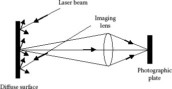
FIGURE 8.1 Schematic for recording a subjective speckle pattern on a photographic plate using an imaging lens.

DSP, also called as speckle correlation (SC), electronic speckle photography (ESP), or digital image correlation (DIC) is the digital/electronic version of speckle photography for the evaluation of displacement fields [5,6,7,8,9,10,11]. A basic DSP system has relatively low complexity in the hardware as the photographic plate is replaced with a CCD camera. The registration of the speckle pattern is made by video/digital recording of the object and the evaluation process is performed on a PC. The analysis is much faster as no film processing or reconstruction (filtering) is needed. The method is based on a cross-correlation analysis of two speckle patterns, one stored before and another after the object is deformed. The method does not follow the movement of each speckle, but rather the movement of a number of speckles acting together as a subimage.

Photorefractive crystals with their unique properties of higher resolution, low intensity operation, and the capability of real-time response have been used to record and analyze the SC fringes [12,13,14,15,16]. The basic concept here is that the two beams interfere inside the photorefractive material and produce a dynamic grating. At the observation plane, one can have two speckle fields: (1) the first one constitutes the initial state of the object, that is, due to the diffraction of the pump beam from the grating formed at the crystal plane, and (2) the second scattered beam that represents the directly transmitted object beam that constitutes the deformed state of the object. The overlap of these two identical but displaced speckles give rise to the SC fringe pattern in real time.

8.3 SPECKLE INTERFEROMETRY

Speckle interferometry is a powerful measurement method involving coherent addition (interference) of the scattered wave from the object surface with a reference wave that may be a specular or scattered field [1]. Unlike speckle photography, this technique has a sensitivity comparable to that of holographic interferometry. The phase changes within one speckle due to the object displacement coded by the reference wave. This displacement is extracted by correlating two speckle patterns one taken before and another after object displacement. Figure 8.2 shows a schematic of a speckle interferometer. Here the speckled image of the object is superposed with the reference beam at the image plane of the imaging lens and they add coherently to form a resultant speckle pattern.

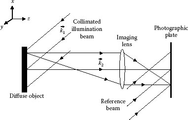
FIGURE 8.2 Schematic of a speckle interferometer.

The irradiance of a speckle pattern at any point in the image plane, before object deformation can be written as

$I_{B} = I_{O} + I_{R} + 2 \sqrt{I_{O} I_{R}} \cos ϕ$ $I_{B} = I_{O} + I_{R} + 2 \sqrt{I_{O} I_{R}} \cos ϕ$

(8.1)

where

I_O and I_R are the irradiances of the object and reference waves, respectively, at the image plane

ϕ is the random phase difference between them

The irradiance at the same point after deforming the object can be written as

$I_{A} = I_{O} + I_{R} + 2 \sqrt{I_{O} I_{R}} \cos (ϕ + Δ ϕ)$ $I_{A} = I_{O} + I_{R} + 2 \sqrt{I_{O} I_{R}} \cos (ϕ + Δ ϕ)$

(8.2)

where Δϕ is the additional phase change introduced due to the object deformation. The total intensity recorded by the double exposure is given by

$I = I_{A} + I_{B} = 2 (I_{O} + I_{R}) + 4 \sqrt{I_{O} I_{R}} \cos (ϕ + \frac{ϕ}{2}) \cos (\frac{Δ ϕ}{2})$ $I = I_{A} + I_{B} = 2 (I_{O} + I_{R}) + 4 \sqrt{I_{O} I_{R}} \cos (ϕ + \frac{ϕ}{2}) \cos (\frac{Δ ϕ}{2})$

(8.3)

The speckle pattern would be unchanged if Δϕ = 2nπ and would be totally de-correlated when Δϕ = (2n + 1)π. The correlated areas appear as bright fringes and uncorrelated areas appear as dark fringes on filtering. The phase change because of object deformation can be expressed as

$Δ ϕ = ({\vec{k}}_{2} - {\vec{k}}_{1}) \cdot \vec{L}$ $Δ ϕ = ({\vec{k}}_{2} - {\vec{k}}_{1}) \cdot \vec{L}$

(8.4)

where ${\vec{k}}_{2}$ ${\vec{k}}_{2}$ and ${\vec{k}}_{1}$ ${\vec{k}}_{1}$ are the propagation vectors in the directions of illumination and observation, respectively, as shown in Figure 8.2. $\vec{L} (u, v, w)$ $\vec{L} (u, v, w)$ is the displacement vector, u, v, and w being the displacement components along x, y, and z directions, respectively. Since the fringes are loci of constant phase difference, the deformation vector components can be measured using appropriate optical configurations.

If one of the surfaces is moved along the line of sight, the speckle pattern undergoes an irradiance change. However, if the surface is displaced through a distance of nλ/2, where n is an integer, λ is the wavelength of the light used, the resultant speckle pattern undergoes a phase change of 2nπ and returns to the original texture. The resultant speckle pattern in the original and the displaced states of the surfaces are correlated. For very large displacements, the correlation property fails to exist, as the whole speckle structure changes.

8.3.1 OUT-OF-PLANE DISPLACEMENT MEASUREMENT

If the displacement varies across the surface of the object, the resultant speckle pattern will remain correlated in the areas where the displacement along the line of sight is an integral multiple of λ/2 (which corresponds to a net change of λ or a phase change of 2π) and they will be uncorrelated in other areas. It is possible to detect these positions of correlation and the interferometer can be used for measuring the change in phase (or the surface movement). A straightforward way to doing this is to adopt the photographic mask method. The resultant speckle pattern is recorded on a photographic plate, and the processed plate is replaced exactly in its original position. Since the processed plate is a negative of the recorded speckle pattern, the dark areas of the plate correspond to bright speckles and vice versa. The overall light transmitted by the plate will thus be very small. If the surface is deformed such that the displacement varies across the surface, the phase change also varies across the surface. The mask will transmits light in those parts of the image where the speckle pattern is not correlated with it, but does not transmit light in correlated area. This gives rise to an apparent fringe pattern covering the image. The fringes are termed as correlation fringes, which are obtained by the addition of two or more speckle patterns. However, we often use subtraction correlation fringes in electronic/digital speckle pattern interferometry (ESPI/DSPI). The phase change can be related to out-of-plane displacement component as Ref. [1]

$Δ ϕ = (\frac{4 π}{λ}) w$ $Δ ϕ = (\frac{4 π}{λ}) w$

(8.5)

A comparative speckle interferometric configuration in which two objects (master and test objects) are compared with each other for nondestructive testing is also reported in literature [17,18].

8.3.2 IN-PLANE DISPLACEMENT MEASUREMENT

Leendertz [1] proposed a novel method for in-plane measurements that consists of symmetrically illuminating the diffuse object under test by two collimated beams at an angle θ on either side of the surface normal as shown in Figure 8.3. If this surface is imaged on to a photographic plate, the image will consist of two independent, coherent speckle patterns due to each beam.

If we assume the illuminating beams to lie symmetrically with respect to normal in the x−z plane, following Equation 8.4 one can write the phase difference as [1]

$Δ ϕ = (\frac{2 π}{λ}) 2 u \sin θ$ $Δ ϕ = (\frac{2 π}{λ}) 2 u \sin θ$

(8.6)

where u is the x-component of the displacement. The arrangement is intrinsically insensitive to the out-of-plane displacement component; the y component (v) is not sensed because of the illumination beams lying in the x−z plane. Physically, the out-of-plane displacement of the object introduces identical path changes in both of the observation beams, and the v component of in-plane displacement does not introduce any path change in either of the observation beams. Bright fringes are formed when

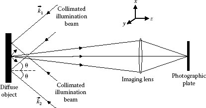
FIGURE 8.3 Leendertz’s arrangement for in-plane displacement measurement.

$2 u \sin θ = m λ$ $2 u \sin θ = m λ$

(8.7)

where m is an integer.

The fringe spacing corresponds to an incremental displacement of λ/2 sin θ. The sensitivity of the setup can be varied by changing the angle between the illuminating beams. The orthogonal component of in-plane displacement (v) can be obtained by rotating either the object or the illuminating beams by 90° about the normal to the object. Further, two pairs of symmetrical beams orthogonal to each other can be used to obtain the u and v components simultaneously. An optical configuration for measuring the in-plane displacement component with twofold sensitivity is also proposed [19,20]. In this arrangement, the object is illuminated symmetrically with two beams, and the observation is made along the same directions of illumination, and combined them at the image plane of the imaging system to yield twofold measuring sensitivity.

A method for measuring in-plane displacement has been described by Duffy [21,22]. It consists of imaging the object surface through a lens fitted with a double aperture located symmetrically with respect to the optical axis as shown in Figure 8.4. The lens focused on the surface sees an arbitrary point on the object surface along two different directions. As a result of the coherent superposition of the beams emerging from the two apertures, each speckle is modulated by a grid structure running perpendicular to the line joining the apertures. The pitch of the fringe system embedded in each speckle depends on the separation of the two apertures. During filtering, the grid structure diffracts light in well-defined directions. Because there is considerably more light available in these halos, there is an enormous gain in the signal-to-noise ratio, resulting in almost unit contrast fringes [23].

The in-plane displacement (u) can be expressed in terms of optical geometry as

$Δ ϕ = (\frac{2 π}{λ}) 2 u \sin α$ $Δ ϕ = (\frac{2 π}{λ}) 2 u \sin α$

(8.8)

Equation 8.8 is similar to Equation 8.6 except that θ is replaced by α. The angle α is governed by the aperture of the lens, and hence the sensitivity of Duffy’s arrangement is inherently poor. Khetan and Chang [23] extended this technique by using four apertures, two along x-axis and two along the y-axis. A modified arrangement for measuring in-plane displacement equal to Leendertz’s dual beam illumination method [1] is also reported [24]. Novelty of the multiaperture methods is in multiplexing using theta modulation or frequency modulation [25]. All these interferometers have been extensively used with electronic/digital speckle interferometry for various applications of optical metrology.

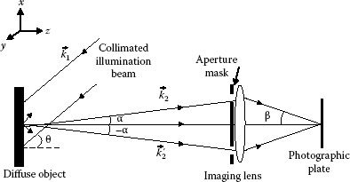
FIGURE 8.4 Duffy’s arrangement for in-plane displacement measurement.

8.4 SPECKLE SHEAR INTERFEROMETRY

Speckle shear interferometry or shearography is also a full-field, noncontact optical technique, usually used for the measurement of changes in the displacement gradient caused by surface and subsurface defects [26,27,28]. It is an optical differentiation technique where the speckle pattern is optically mixed with an identical but displaced, or sheared, speckle pattern using a shearing device, and viewed through a lens, forming a speckle shear interferogram at the image plane. It is analogous to the conventional shear interferometry where two sheared wavefronts are made to interfere in order to measure the rate of change of phase across the wavefront. A double exposure record is made with the object displaced between the exposures. The correlation fringes formed on filtering provide displacement gradient in the shear direction. This is a more useful data for experimental stress analysis as this quantity is proportional to the strain.

8.4.1 SLOPE MEASUREMENT

Speckle shear interferometry is useful for measurement of first-order derivative of the out-of-plane displacement or the slope. Figure 8.5 shows the optical configuration of the speckle shear interferometer for slope measurement. It is a Michelson interferometer, where a collimated laser beam is used for object illumination. A lateral shear is introduced between the images by tilting the mirror M₂. Assuming a shear Δx in the x-direction, any point in the image plane receives contributions from the neighboring object points (x, y) and (x + Δx, y). The phase change due to object deformation can be written as

$Δ ϕ = Δ ϕ_{2} - Δ ϕ_{1}$ $Δ ϕ = Δ ϕ_{2} - Δ ϕ_{1}$

(8.9)

where Δϕ₁ and Δϕ₂ are the phase changes occurring due to object deformation at the two sheared object points.

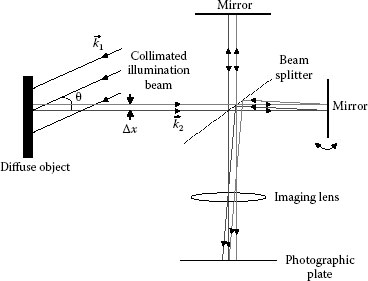
FIGURE 8.5 Speckle shear interferometer for slope measurement.

The phase changes Δϕ₁ and Δϕ₂ are defined by

$Δ ϕ_{1} = ({\vec{k}}_{2} - {\vec{k}}_{1}) \cdot \vec{L}$ $Δ ϕ_{1} = ({\vec{k}}_{2} - {\vec{k}}_{1}) \cdot \vec{L}$

(8.10)

$Δ ϕ_{2} = ({\vec{k}}_{2} - {\vec{k}}_{1}) \cdot {\vec{L}}^{'}$ $Δ ϕ_{2} = ({\vec{k}}_{2} - {\vec{k}}_{1}) \cdot {\vec{L}}^{'}$

(8.11)

where

$\vec{L} = \vec{L} (u, v, w)$ $\vec{L} = \vec{L} (u, v, w)$ and ${\vec{L}}^{'} = \vec{L} (u + Δ u, v + Δ v, w + Δ w)$ ${\vec{L}}^{'} = \vec{L} (u + Δ u, v + Δ v, w + Δ w)$ are the deformation vectors at the points (x, y) and (x + Δx, y), respectively

${\vec{k}}_{1}$ ${\vec{k}}_{1}$ and ${\vec{k}}_{2}$ ${\vec{k}}_{2}$ are the wave vectors in the illumination and observation directions, respectively

If the illumination angle is θ, then the phase change Δϕ can be written as

$Δ ϕ = \frac{2 π}{λ} [\frac{\partial u}{\partial x} \sin θ + \frac{\partial w}{\partial x} (1 + \cos θ)] Δ x$ $Δ ϕ = \frac{2 π}{λ} [\frac{\partial u}{\partial x} \sin θ + \frac{\partial w}{\partial x} (1 + \cos θ)] Δ x$

(8.12)

For normal illumination, θ = 0, the phase can be related to first-order derivative of out-of-plane displacement component (w) as

$Δ ϕ = \frac{4 π}{λ} \frac{\partial w}{\partial x} Δ x$ $Δ ϕ = \frac{4 π}{λ} \frac{\partial w}{\partial x} Δ x$

(8.13)

Thus the fringes formed are contours of ∂w/∂x. Similarly by introducing a shear along y-direction, ∂w/∂y fringes can be obtained.

Multiaperture speckle shear interferometry is also used for slope measurement [28]. The main advantages of image plane shear using multiaperture arrangements are (1) large depth of focus/field, (2) the interferograms of unit contrast, and (3) its ability to store and retrieve multiple information pertaining to partial derivatives of an object deformation from a single specklegram. Further, the setups are inexpensive, simple, and require little vibration isolation. The limitations of these interferometers are that they are intrinsically sensitive to both the in-plane displacement component and its derivatives. The fringe pattern thus contains information of (1) in-plane displacement, (2) its derivative, and (3) the derivative of the out-of-plane displacement component (slope) [28,29,30]. Apart from lateral shear, radial, rotational, inversion, and folding shear have also been introduced in speckle shear interferometry [28].

8.4.2 CURVATURE MEASUREMENT

For plate bending problems and flexural analysis, the second-order derivatives of the out-of-plane displacements are required for calculating the stress components. Hence it is necessary to perform differentiation of the slope data to obtain curvature information. Multiple aperture configurations [31,32] can yield curvature information by proper filtering of the halos. The configuration is shown in Figure 8.6, where a plate with three holes drilled in a line is used as a mask in front of the imaging lens. Two identical small angled wedges are placed in front of the two outer apertures, while a suitable flat glass plate is placed in front of the central aperture to compensate for the optical path. Each point on the image plane gets contribution from three neighboring points on the object. Thus, three different processes of coherent speckle addition take place simultaneously in the interferometer. As a result, the speckle pattern is modulated by three systems of grid structures running perpendicular to the lines joining the apertures. Two exposures are made of the object illuminated with laser light, once before and once after loading. When subjected to Fourier filtering, the double exposed speckle shearogram results in five diffraction halos in the Fourier plane. By filtering the first-order halos one can get the curvature fringes as Moiré pattern [31]. The information along any other direction can be obtained by orienting the wedge device along that particular direction.

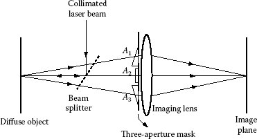
FIGURE 8.6 Three-aperture speckle shear interferometer for curvature measurement.

The holographic optical elements (HOEs) are also extensively used in speckle interferometry and speckle shear interferometry configurations for the measurement of displacement and its derivatives [33,34,35].

8.5 DIGITAL SPECKLE AND SPECKLE SHEAR INTERFEROMETRY

The average speckle size is typically in the range 5–100 μm. A standard television (TV) camera can therefore be used to record the intensity pattern instead of a photographic plate. The video processing of the signal may be used to generate SC fringes equivalent to those obtained by photographic processing. The suggestion of replacing the photographic plate with a detector and an image processing unit for real-time visualization of correlation speckle fringes was first reported by Leendertz and Butters [36]. This pioneering contribution is today referred in literature as ESPI, DSPI, phase-shifting speckle interferometry (PSSI), or TV holography (TVH) [37,38,39,40]. Starting from these basic ideas, contributions on various refinements, extensions, and novel developments have been proposed. They have continued to pour in over the years from researchers across the globe, and have contributed to the gradual evolution of the concept into a routinely used reliable and versatile technique for quantitative measuring displacement components of a deformation vector of diffusely scattering object under static or dynamic load. The ability to measure 3D surface profiles by generating contours of constant depth of an object is yet another major achievement of DSPI. The last three decades have seen a significant increase in the breadth and scope of applications of DSPI in areas such as experimental mechanics, vibration analysis, nondestructive testing, and evaluation. Digital shearography (DS) or digital speckle shear pattern interferometry (DSSPI) is an outgrowth of speckle shear interferometry in concept, and involves optical and electronic principle akin to those used in DSPI [38]. It has been widely used for measuring the derivatives of surface displacements of rough objects undergoing deformation. The method has found a prominent use for nondestructive testing of structures. Digital/electronic speckle and speckle shear configurations have been combined with phase-shifting interferometry (PSI) [41] for a wide range of quantitative data analysis of engineering structures.

8.5.1 FRINGE ANALYSIS

Figure 8.7 represents widely used in-line DSPI arrangement for the measurement of out-of-plane displacement. The beam from a laser source is split into an object beam and a reference beam. The scattered object beam is combined with a reference beam using a beam splitter (BS) at the CCD plane. The complex amplitudes of the object, A_O and the reference, A_R beams at any point (x, y) on the CCD array can be expressed as

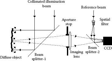
$A_{O} (x, y) = a_{O} (x, y) \exp [i ϕ_{O} (x, y)]$ $A_{O} (x, y) = a_{O} (x, y) \exp [i ϕ_{O} (x, y)]$

(8.14)

FIGURE 8.7 DSPI arrangement sensitive to out-of-plane displacement.

and

$A_{R} (x, y) = a_{R} (x, y) \exp [i ϕ_{R} (x, y)]$ $A_{R} (x, y) = a_{R} (x, y) \exp [i ϕ_{R} (x, y)]$

(8.15)

where

a_O(x, y) is the amplitude

ϕ_O(x, y) is the phase of the light scattered from the object in its initial state

a_R(x, y) is the amplitude

ϕ_R(x, y) is the phase of the reference beam

The irradiance at any point (x, y) on the CCD array can be expressed as

$\begin{array}{l} I_{B} (x, y) & = {| A_{O} (x, y) + A_{R} (x, y) |}^{2} \\ = {| A_{O} (x, y) |}^{2} + {| A_{R} (x, y) |}^{2} + 2 | A_{O} (x, y) | | A_{R} (x, y) | \cos [ϕ_{B} (x, y)] \\ = I_{O} (x, y) + I_{R} (x, y) + 2 \sqrt{I_{O} (x, y) I_{R} (x, y)} \cos [ϕ_{B} (x, y)] \end{array}$ $\begin{array}{l} I_{B} (x, y) & = {| A_{O} (x, y) + A_{R} (x, y) |}^{2} \\ = {| A_{O} (x, y) |}^{2} + {| A_{R} (x, y) |}^{2} + 2 | A_{O} (x, y) | | A_{R} (x, y) | \cos [ϕ_{B} (x, y)] \\ = I_{O} (x, y) + I_{R} (x, y) + 2 \sqrt{I_{O} (x, y) I_{R} (x, y)} \cos [ϕ_{B} (x, y)] \end{array}$

(8.16)

where

ϕ_B(x, y) = ϕ_O(x, y) − ϕ_R(x, y) represents the random speckle phase

I_O(x, y) and I_R(x, y) are the irradiances of the object and reference beams, respectively

Assuming the output camera signal to be proportional to the irradiance, the video signal is then

$ν_{B} \propto I_{B} (x, y)$ $ν_{B} \propto I_{B} (x, y)$

(8.17)

The analog video signal ν_B from the CCD is sent to an analog-to-digital converter, which samples the video signal at the TV rate and records it as a digital frame in the memory of a computer for subsequent processing.

If the object is deformed, the relative phase of the two fields will change, thus causing a variation in the irradiance of the speckle pattern. The deformation gradients applied on the object surface are assumed to be small. Following the application of the load, the complex amplitude of the object wavefront can be expressed as

${A^{'}}_{O} (x, y) = a_{O} (x, y) \exp {i [ϕ_{O} (x, y) + Δ ϕ (x, y)]}$ ${A^{'}}_{O} (x, y) = a_{O} (x, y) \exp {i [ϕ_{O} (x, y) + Δ ϕ (x, y)]}$

(8.18)

where Δϕ(x, y) is the phase difference introduced in the original object beam due to object deformation.

The irradiance distribution after object deformation can be written as

$I_{A} (x, y) = I_{O} (x, y) + I_{R} (x, y) + 2 \sqrt{I_{O} (x, y) I_{R} (x, y)} \cos [ϕ_{A} (x, y)]$ $I_{A} (x, y) = I_{O} (x, y) + I_{R} (x, y) + 2 \sqrt{I_{O} (x, y) I_{R} (x, y)} \cos [ϕ_{A} (x, y)]$

(8.19)

where ϕ_A(x, y) = ϕ_B(x, y) + Δϕ(x, y) − Φ_R(x, y).

A common method to produce SC fringes is based on direct electronic subtraction of the intensities in the initial and deformed states of the object. The video signal ν_A is digitized and then subtracted from the digital frame corresponding to ν_B.

The subtracted video signal ν is then given by

$ν = (ν_{A} - ν_{B}) \propto (I_{A} - I_{B}) = Δ I = 4 \sqrt{I_{O} I_{R}} \sin (ϕ_{B} + \frac{Δ ϕ}{2}) \sin (\frac{Δ ϕ}{2})$ $ν = (ν_{A} - ν_{B}) \propto (I_{A} - I_{B}) = Δ I = 4 \sqrt{I_{O} I_{R}} \sin (ϕ_{B} + \frac{Δ ϕ}{2}) \sin (\frac{Δ ϕ}{2})$

(8.20)

This signal has both positive and negative values. The TV monitor, however, displays the negative going signals as black areas. To avoid this loss of signal, it is rectified before being displayed on the monitor. The brightness on the monitor is then proportional to |ΔI| and can be expressed as

$B = C | Δ I | = C | 4 \sqrt{I_{O} I_{R}} \sin (ϕ_{B} + \frac{Δ ϕ}{2}) \sin (\frac{Δ ϕ}{2}) |$ $B = C | Δ I | = C | 4 \sqrt{I_{O} I_{R}} \sin (ϕ_{B} + \frac{Δ ϕ}{2}) \sin (\frac{Δ ϕ}{2}) |$

(8.21)

where C is a proportionality constant. The term (ϕ_B + Δϕ/2) represents the speckle noise which varies randomly between 0 and 1. Equation 8.21 describes the modulation of the high-frequency noise by a low-frequency interference pattern related to the phase-difference term Δϕ.

The brightness will be minimized when

$Δ ϕ = 2 n π, n = 0, 1, 2, …$ $Δ ϕ = 2 n π, n = 0, 1, 2, …$

(8.22)

This condition corresponds to dark fringe and denotes all of those regions where the speckle patterns, both before and after deformation, are correlated. On the other hand, the brightness will be maximized when

$Δ ϕ = (2 n + 1) π, n = 0, 1, 2, …$ $Δ ϕ = (2 n + 1) π, n = 0, 1, 2, …$

(8.23)

This condition corresponds to bright fringe and denotes all of those regions where the speckle patterns, both before and after deformation, are uncorrelated. As a result, SC fringes representing contours of constant displacement are seen to appear on the monitor in the form of bright and dark bands modulating the object image.

For in-plane displacement and slope measurements, the configurations shown in Figures 8.3 and 8.5 are widely adopted by replacing the photographic plate with a CCD. Figure 8.8a and b shows the real-time out-of-plane and slope correlation fringes from a rigidly clamped circular diaphragm loaded at the center.

The procedure described above provides the qualitative analysis of the fringes. It is, in general, impossible to obtain a unique phase distribution from a single interferogram. For example, substitution of −ϕ_A for ϕ_A in Equation 8.19 results in the same intensity map, indicating that positive displacement cannot be distinguished from negative displacements without further information. The near-universal technique of solving this problem is to add to the phase function a known phase ramp, or carrier, which is linear in either time or position. In the former case, the resulting intensity distributions are sampled at discrete time intervals and the technique is known as temporal phase shifting (TPS) [41]; in the latter case, a single intensity distribution is sampled at discrete points in the image, in which case it is referred to as spatial phase shifting (SPS) [42]. TPS technique involves introduction of an additional controlled phase change, ϕ₀, between the object and reference beams. Normally a linear ramp ϕ₀ = αt, is used, where α represents the phase shift introduced between two successive frames, and t is the time variant [43,44]. Equation 8.16 then becomes

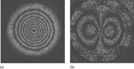
FIGURE 8.8 SC fringe patterns obtained for a rigidly clamped circular diaphragm loaded at the center from (a) DSPI arrangement and (b) DS arrangement.

$I_{B} (x, y) = I_{O} (x, y) + I_{R} (x, y) + 2 \sqrt{I_{O} (x, y) I_{R} (x, y)} \cos [ϕ_{B} (x, y) + α t]$ $I_{B} (x, y) = I_{O} (x, y) + I_{R} (x, y) + 2 \sqrt{I_{O} (x, y) I_{R} (x, y)} \cos [ϕ_{B} (x, y) + α t]$

(8.24)

Equation 8.24 can also be written as

$I_{B} (x, y) = I_{b} (x, y) + γ (x, y) cos [ϕ_{B} (x, y) + α t]$ $I_{B} (x, y) = I_{b} (x, y) + γ (x, y) cos [ϕ_{B} (x, y) + α t]$

(8.25)

where

I_b = I_O + I_R is the bias intensity

$γ = 2 \sqrt{I_{O} I_{R}}$ $γ = 2 \sqrt{I_{O} I_{R}}$ is the visibility of the interference pattern

The temporal phase-shifting technique involves analyzing data from each pixel independently of all of the other pixels in the image, using different phase-shifting algorithms.

Most widely used algorithm for phase calculation is the four-step algorithm [38,45]. A π/2 phase shift is introduced into the reference beam between each of the sequentially recorded interferograms. So ϕ₀ now takes on four discrete values as ϕ₀ = 0, π/2, π, 3π/2. Substituting each of these four values into Equation 8.25 results in four equations describing the four measured intensity patterns as

$I_{1} = I_{b} + γ \cos ϕ_{B}$ $I_{1} = I_{b} + γ \cos ϕ_{B}$

(8.26)

$I_{2} = I_{b} + γ \sin ϕ_{B}$ $I_{2} = I_{b} + γ \sin ϕ_{B}$

(8.27)

$I_{3} = I_{b} + γ \cos ϕ_{B}$ $I_{3} = I_{b} + γ \cos ϕ_{B}$

(8.28)

$I_{4} = I_{b} + γ \sin ϕ_{B}$ $I_{4} = I_{b} + γ \sin ϕ_{B}$

(8.29)

The phase ϕ thus can be calculated as

$ϕ_{B} = \arctan (\frac{I_{2} - I_{4}}{- I_{1} + I_{3}})$ $ϕ_{B} = \arctan (\frac{I_{2} - I_{4}}{- I_{1} + I_{3}})$

(8.30)

A phase-shifting algorithm that is less sensitive to reference phase-shift calibration errors is provided by Hariharan et al. [46]. The phase ϕ_B can be obtained from

$ϕ_{B} = \arctan (\frac{2 (I_{2} - I_{4})}{- I_{1} + 2 I_{3} - I_{5}})$ $ϕ_{B} = \arctan (\frac{2 (I_{2} - I_{4})}{- I_{1} + 2 I_{3} - I_{5}})$

(8.31)

The subtraction of the phase obtained before (ϕ_B) and after loading (ϕ_A) the object yields the phase map Δϕ related to object deformation [37].

The most common method used to introduce the phase shift in a PSI is to translate one of the mirrors in the interferometer with a piezoelectric translator. Piezoelectric translator consists of lead–zirconium–titanate (PZT) or other ceramic materials, which expand or contract with an externally applied voltage. Shifts from submicrometer to several micrometers can be achieved using PZT. However, the miscalibration, nonlinearity, and hysteresis of PZTs are the error sources, which influence the accuracy of the phase measurements [47,48]. Polarization components such as rotating half-wave plate (HWP), quarter-wave plate (QWP), and polarizers are also used as phase shifters [49]. The other schemes available for introducing phase shifts are liquid crystal phase shifters, source wavelength modulation [37,50], air-filled quartz cell [51], etc.

Spatial phase-shifting technique provides a useful alternative to TPS when dynamic events are being investigated, or when vibration is a problem, because all the data needed to calculate a phase map are acquired at the same instant [42]. Since the phase shift then has to take place in space instead of time, this approach is quite generally called SPS. In principle, it gets possible to track the object phase at the frame rate of the camera, with the additional benefit that any frame of the series can be assigned the new reference image.

A simpler technique involves recording of just two images, once before and once after the object deformation, in which a spatial carrier is introduced within the speckle. The time variation in Equation 8.25 is then replaced by the following spatial variation:

$I_{B} (x, y) = I_{b} (x, y) + γ (x, y) \cos [ϕ_{B} (x, y) + α x]$ $I_{B} (x, y) = I_{b} (x, y) + γ (x, y) \cos [ϕ_{B} (x, y) + α x]$

(8.32)

In the case of out-of-plane displacement, the simplest way of generating a carrier fringe within a speckle with a linear variation is to use off-axis reference wave with a small angular offset between the object and reference beams, unlike the conventional DSPI system [52,53]. The spatial carrier is apparent as grid-like structure, and the random variations in speckle to speckle manifest themselves as lateral shifts of the carrier. It is common to set the carrier fringe so that there is a 90° or 120° phase shift between the adjacent pixels of the CCD detector and to use three or more adjacent pixels to evaluate the phase of the interference. The alternative approach to generate the spatial carrier fringe is by adopting a double aperture mask in front of the imaging system [54,55] as shown in Figure 8.4.

The “phase-of-differences” method [37] represents a useful way of generating visible phase-shifted fringe patterns. There is an alternative method known as “difference-of-phases,” where the phase ϕ evaluated from the phase shifted “before” load images is subtracted from the phase ϕ + Δϕ evaluated from the phase shifted “after” load images to yield the phase Δϕ [37,38]. As the calculated phase values lie in the principle range (−π, π), Δϕ lies in the range (−2π, 2π). This would normally be wrapped back on to the range [56]. The phase-change distribution Δϕ due to object deformation obtained from Equation 8.30 or 8.31 yields only a sawtooth function showing the phase modulo 2π. These 2π phase jumps can be eliminated by using the phase unwrapping method [56,57] so that a continuous function of the relative phase change Δϕ, i.e., the unwrapped phase map, is generated. The phase unwrapping method can be performed only for a noise reduced sawtooth image. As a result of electronic and optical noise mainly due to speckle decorrelation effects, it is difficult to distinguish between real phase jumps, and jumps due to noise because they fulfill the same mathematical requirements. Consequently, there must be a relationship between phase edge preservation and noise removal in the design of the filter. Many filtering techniques have been proposed to condition the phase map before the application of the unwrapping procedure [56,57]. The known filter operations in the field of digital image processing can be broadly classified into two categories: those used for linear operations, i.e., low-pass filtering or average filtering, and for nonlinear operations, for example, median filtering. Since both the speckle noise and the 2π discontinuities in phase fringe patterns are characterized by high spatial frequencies, applying a filter not only reduces the noise but also smears out the discontinuities. This problem is solved by calculating the sine and cosine of the wrapped phase map Δϕ, which leads to the continuous fringe patterns sin Δϕ and cos Δϕ and then applying filtering, known as sine–cosine filtering scheme [58]. Another interesting type of filter is the phase filter [38] that is a modified version of average filter. There are many other sophisticated filters like scale-space filter [59], adaptive median filter [60], special averaging filter [61], and histogram-data-orientated filter [62], in making noise reduced phase map before unwrapping. All the filters have relative merits and demerits, and usefulness of a particular filter depends upon the application.

Unwrapping is the procedure which removes these 2π phase jumps and the result is converted into desired continuous phase function, thus phase unwrapping is an important final procedure for DSPI fringe analysis process. The process is carried out by adding or subtracting 2π each time the phase map presents a discontinuity. Even though these methods are well suited for unwrapping noise-free data, the process becomes more difficult when the absolute phase difference between the adjacent pixels with no discontinuities is greater than π. These spurious jumps may be caused by noise, discontinuous phase jumps, and regional under-sampling in the fringe pattern. If any of such local phase inconsistencies are present, an error appears which is propagated along the unwrapping path. To avoid this problem, sophisticated algorithms have been proposed [57]. These methods include unwrapping by the famous branch-cut technique [63] and with discrete cosine transform (DCT) [64]. The former method detects error inducing locations in the phase map and connects them to each other by a branch-cut, which must not be crossed by a subsequent unwrapping with a simple path dependent method. The DCT approaches the problem of unwrapping by solving the Poisson equation relating wrapped and unwrapped phases by 2D DCT. This way, any path dependency is evaded and error propagation does not appear “localized” as for scanning methods. The advantage of this technique is that noise in wrapped data has less influence, and that the whole unwrapping is performed in a single step (no step function is created), though the time consumed is rather high compared to path dependent methods. The multigrid algorithm is an iterative algorithm that adopts a recursive mode of operation and forms the basis for most multigrid algorithms [57,65]. Multigrid methods are a class of techniques for rapidly solving partial differential equations (PDEs) on large grids. These methods are based on the idea of applying Gauss–Seidel relaxation schemes on coarser, smaller grids. After application of any phase unwrapping algorithm, “true” phase jumps in unwrapped phase data higher than 2π cannot be identified correctly, as these are interpreted as changes of order. Figure 8.9 shows the speckle fringe analysis on a centrally loaded, rigidly clamped circular diaphragm using the TPS “difference-of-phases” method [37] and DCT unwrapping algorithm [57].

8.5.2 OPTICAL SYSTEMS IN DIGITAL SPECKLE AND SPECKLE SHEAR INTERFEROMETRY

Several optical systems in digital speckle and speckle shear interferometry have also been developed for the measurement of displacement and its derivates [37,38]. For measurement of the out-of-plane displacement component of a deformation vector, the optical systems are based on either (1) in-line reference wave [66,67] or (2) off-axis reference wave [68,69]. A desensitized system for large out-of-plane displacement is also reported [70,71,72]. Further, portable systems have been reported with the possibility for the system to be implemented in remote conditions [73,74,75,76,77].

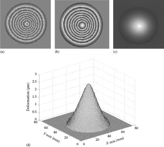
FIGURE 8.9 Speckle fringe analysis using temporal phase shifting “difference-of-phases” method: (a) raw phase map, (b) filtered phase map, (c) corresponding unwrapped 2D, and (d) 3D plots of the out-of-plane displacement.

For in-plane displacement measurement, Leendertz’s dual beam illumination and normal observation configuration are widely adopted (Figure 8.3). The other configurations emerged in recent years are (1) oblique illumination–observation [78], (2) normal illumination–dual direction observation [79], and (3) dual beam symmetric illumination–observation [79,80,81,82,83,84]. The dual beam symmetric illumination–observation systems had an additional advantage of measuring the in-plane displacement component with twofold sensitivity [82,83,84]. The in-plane sensitive systems are also used to determine the shape or surface profile of the 3D objects [37]. Some novel systems for evaluating displacement components from a single optical head are also described [85,86,87,88].

Digital speckle shear interferometry or DS has been widely used for the measurement of the spatial derivatives of object deformation. The DS system has found a prominent application in aerospace industry for nondestructive testing of spacecraft structures [89,90,91]. A Michelson-type of shear interferometer as shown in Figure 8.5 is extensively employed to introduce lateral shear in an optical configuration [92,93,94,95]. NDE analysis on a polymethyl methacrylate (PMMA) panel clamped at the bottom and subjected to thermal stressing using DS is shown in Figure 8.10. A universal shear interferometer has been proposed to implement lateral, radial, rotational, and inversion shear evaluations [96]. Dual-beam symmetric illumination in a Michelson shear arrangement for obtaining the partial derivatives of in-plane displacements (strain) is also reported [97,98,99]. The other prominent shearing devices reported are split lens shear element [100], birefringent crystals [101,102], and HOE such as holo-shear lens (HSL) [103] and holo-gratings (HG) [104]. Waldner and Brem [105] developed a portable, compact shearography system. A multiwavelength DS is also reported for extracting the in-plane and out-of-plane strains from a single system [106,107]. A large area composite helicopter structures for non destructive testing (NDT) inspection is also examined by Pezzoni and Krupka [108], to show the potential application of the shearography for large size structures. Of the many salient developments, the two that one could probably cite here concern the measurement of out-of-plane displacement and their derivatives [109,110,111,112,113,114,115], and the measurement of second-order partial derivatives [116,117] of out-of-plane displacement (curvature and twist). The shearography is also exploited for slope contouring of 3D objects either by varying the refractive index, wavelength, or rotation of the 3D surface between the frames [118,119,120].

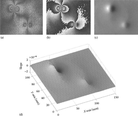
FIGURE 8.10 NDE of PMMA panel subjected to thermal stressing with DS: (a) fringe pattern, (b) filtered phase map, (c) 2D plot, and (d) 3D plots of the slope.

8.5.3 APPLICATION TO MICROSYSTEMS ANALYSIS

Microsystems such as MEMS and micro-opto-electromechanical systems (MOEMS) combining micro-size electrical and mechanical mechanism are finding increasing applications in various fields. In recent years, the technology of fabricating MEMS has been adopted by a number of industries to produce sensors, actuators, visual display components, AFM probe tips, semiconductor devices, etc. Aided by photolithography and other novel methods, large number of MEMS devices are fabricated simultaneously. So, high-quality standards are a must for the manufacturers in MEMS technology. The materials behavior in combination with new structural design cannot be predicted by theoretical simulations. A possible reason for wrong predictions made by finite element method (FEM) and other model analysis with respect to the loading conditions or in practical applications of microdevices is, for instance, the lack of reliable materials data and boundary conditions in microscale. The MEMS devices require measurement and inspection techniques that are fast noncontact and robust. The reasons for such a technology is obvious, properties determined on much larger specimens cannot be scaled down from the bulk material without any experimental evaluation. Further on, in microstructures, the materials behavior is noticeably affected by the production technology. Therefore, simple and robust optical measuring methods to analyze the shape and deformation of the microcomponents under static and dynamic conditions are highly desired [121]. The optical measuring system for the inspection and characterization of M(O)EMS should have the following conditions. First, it should not alter the integrity and the mechanical behavior of the device. Since the microcomponents have an overall size up to a millimeter, a high spatial resolution measuring system is required. The measuring system should be able to perform both static and dynamic measurements. As the deflections, motions, or vibration amplitudes of MEMS are typically in the nanometer to a few microns range, high sensitivity optical methods are highly desired. Finally, the measurement must be quantitative and reliable with a low sensitivity to environmental conditions. Microscopic systems for microcomponents analysis are mostly dependent on the optical system such as long working distance microscope with the combination of different magnification objective lens. Lokberg et al. [122] proposed feasibility of microscopic system on microstructures. Various microscopic imaging systems have been developed for microsystems characterization [123,124,125,126,127,128]. A schematic diagram of a microscopic digital speckle interferometric system is shown in Figure 8.11. In this arrangement, the collimated laser beam illuminates the object and a PZT-driven reference mirror via a cube BS. The scattered object wave from the microspecimen and the smooth reference wave are recombined coherently onto the CCD plane via the same cube BS and the microscopic imaging system. As an example, Figure 8.12 shows the application of the microscopic digital speckle interferometric system for deflection characterization on a MEMS pressure sensor. An endoscopic DSPI system is also reported in literature to study intracavity inspection of biological specimen such as in vitro and in vivo (porcine stomach, mucous membrane) [129,130,131].

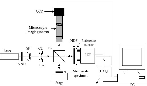
FIGURE 8.11 Schematic of a microscopic DSPI system.

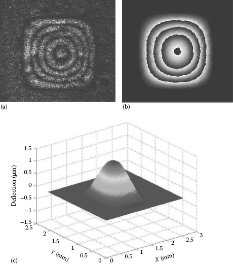
FIGURE 8.12 MEMS (15 mm²) pressure sensor subjected to pressure load: (a) fringe pattern, (b) wrapped phase map, and (c) 3D plot.

8.6 CONCLUSIONS

The chapter covers the speckle methods and their applications to optical metrology. Speckle methods can be broadly classified into three categories: speckle photography, speckle interferometry, and speckle shear interferometry (shearography). The digital speckle methods with high-speed cameras and modern imaging processing systems will find a widespread use in the field of microsystem engineering, aerospace engineering, biological and medical sciences.

REFERENCES

1. Leendertz, J.A., Interferometric displacement measurement on scattering surfaces utilizing speckle effect, J. Phys. E: Sci. Instrum., 3, 214–218, 1970.

2. Archbold, E., Burch, M., and Ennos, A.E., Recording of in-plane surface displacement by double-exposure speckle photography, Opt. Acta, 17, 883–889, 1992.

3. Archbold, E. and Ennos, A.E., Displacement measurement from double exposure laser photographs, Opt. Acta, 19, 253–271, 1992.

4. Khetan, R.P. and Chang, F.P., Strain analysis by one-beam laser speckle interferometry. 1. Single aperture method, Appl. Opt., 15, 2205–2215, 1976.

5. Sutton, M.A., Wolters, W.J., Peters, W.H., Ranson, W.F., and McNeill, S.R., Determination of displacements using an improved digital correlation method, Image Vision Comput., 1, 133–139, 1983.

6. Chen, D.J. and Chiang, F.P., Optimal sampling and range of measurement in displacement-only laser-speckle correlation, Exp. Mech., 32, 145–153, 1992.

7. Noh, S. and Yamaguchi, I., Two-dimensional measurement of strain distribution by speckle correlation, Jpn. J. Appl. Phys., 31, L1299–L1301, 1992.

8. Sjödahl, M. and Benckert, L.R., Electronic speckle photography analysis of an algorithm giving the displacement with sub pixel accuracy, Appl. Opt., 32, 2278–2284, 1993.

9. Sjödahl, M. and Benckert, L.R., Systematic and random errors in electronic speckle photography, Appl. Opt., 33, 7461–7471, 1994.

10. Sjödahl, M., Electronic speckle photography: Increased accuracy by non integral pixel shifting, Appl. Opt., 33, 6667–6673, 1994.

11. Andersson, A., Krishna Mohan, N., Sjödahl, M., and Molin, N.-E., TV shearography: Quantitative measurement of shear magnitudes using digital speckle photography, Appl. Opt., 39, 2565–2568, 2000.

12. Tiziani, H.J., Leonhardt, K., and Klenk, J., Real-time displacement and tilt analysis by a speckle technique using Bi12SiO20 crystal, Opt. Commun., 34, 327–331, 1980.

13. Liu, L., Helmers, H., and Hinsch, K.D., Speckle metrology with novelty filtering using photorefractive two-beam coupling in BaTiO3, Opt. Commun., 100, 301–305, 1993.

14. Sreedhar, P.R., Krishna Mohan, N., and Sirohi, R.S., Real-time speckle photography with two-wave mixing in photorefractive BaTiO3 crystal, Opt. Eng., 33, 1989–1995, 1994.

15. Krishna Mohan, N. and Rastogi, P.K., Phase shift calibration in speckle photography—A first step to practical real time analysis of speckle correlation fringes, J. Mod. Opt., 50, 1183–1188, 2003.

16. Krishna Mohan, N. and Rastogi, P.K., Phase shifting whole field speckle photography technique for the measurement of object deformations in real-time, Opt. Lett., 27, 565–567, 2002.

17. Joenathan, C., Ganesan, A.R., and Sirohi, R.S., Fringe compensation in speckle interferometry—Application to non destructive testing, Appl. Opt., 25, 3781–3784, 1986.

18. Rastogi, P.K. and Jacquot, P., Measurement of difference deformation using speckle interferometry, Opt. Lett., 12, 596–598, 1987.

19. Sirohi, R.S. and Krishna Mohan, N., In-plane displacement measurement configuration with twofold sensitivity, Appl. Opt., 32, 6387–6390, 1993.

20. Krishna Mohan, N., Measurement of in-plane displacement with twofold sensitivity using phase reversal technique, Opt. Eng., 38, 1964–1966, 1999.

21. Duffy, D.E., Moiré gauging of in-plane displacement using double aperture imaging, Appl. Opt., 11, 1778–1781, 1972.

22. Duffy, D.E., Measurement of surface displacement normal to the line of sight, Exp. Mech., 14, 378–384, 1974.

23. Khetan, R.P. and Chang, F.P., Strain analysis by one-beam laser speckle interferometry. 2. Multiaperture aperture method, Appl. Opt., 18, 2175–2186, 1979.

24. Sirohi, R.S., Krishna Mohan, N., and Santhanakrishnan, T., Optical configurations for measurement in speckle interferometry, Opt. Lett., 21, 1958–1959, 1996.

25. Joenathan, C., Mohanty, R.K., and Sirohi, R.S., Multiplexing in speckle shear interferometry, Opt. Acta, 31, 681–692, 1984.

26. Leendertz, J.A. and Butters, J.N., An image-shearing speckle pattern interferometer for measuring bending moments, J. Phys. E: Sci. Instrum., 6, 1107–1110, 1973.

27. Hung, Y.Y. and Taylor, C.E., Speckle-shearing interferometric camera—A tool for measurement of derivatives of surface displacement, Proc. SPIE, 41, 169–175, 1973.

28. Sirohi, R.S., Speckle shearing interferometry—A review, J. Opt., 33, 95–113, 1984.

29. Krishna Mohan, N. and Sirohi, R.S., Fringe formation in multiaperture speckle shear interferometry, Appl. Opt., 35, 1617–1622, 1996.

30. Krishna Mohan, N., Double and multiple-exposure methods in multi-aperture speckle shear interferometry for slope and curvature measurement, Proceedings of Laser Metrology for Precision Measurement and Inspection in Industry, Florianópolis, Brazil, Module 4, Holography and Speckle Techniques, pp. 4.87–4.98, 1999.

31. Sharma, D.K., Sirohi, R.S., and Kothiyal, M.P., Simultaneous measurement of slope and curvature with a three-aperture speckle shearing interferometer, Appl. Opt., 23, 1542–1546, 1984.

32. Sharma, D.K., Krishna Mohan, N., and Sirohi, R.S., A holographic speckle shearing technique for the measurement of out-of-plane displacement, slope and curvature, Opt. Commun., 57, 230–235, 1986.

33. Shaker, C. and Rao, G.V., Speckle metrology using hololenses, Appl. Opt., 23, 4592–4595, 1984.

34. Joenathan, C., Mohanty, R.K., and Sirohi, R.S., Hololenses in speckle and speckle shear interferometry, Appl. Opt., 24, 1294–1298, 1985.

35. Joenathan, C. and Sirohi, R.S., Holographic gratings in speckle shear interferometry, Appl. Opt., 24, 2750–2751, 1985.

36. Leendertz, J.N. and Butters, J.N., Holographic and video techniques applied to engineering measurements, J. Meas. Control., 4, 349–354, 1971.

37. Rastogi, P.K., Ed., Digital Speckle Pattern Interferometry and Related Techniques, John Wiley, Chichester, U.K., 2001.

38. Steinchen, W. and Yang, L., Digital Shearography: Theory and Application of Digital Speckle Pattern Shearing Interferometry, PM100, SPIE, Optical Engineering Press, Washington, DC, 2003.

39. Doval, A.F., A systematic approach to TV holography, Meas. Sci. Technol., 11, R1–R36, 2000.

40. Krishna Mohan, N., Speckle techniques for optical metrology, in Progress in Laser and Electro-Optics Research, Arkin, W.T., Ed., Nova Science Publishers Inc., New York, 2006, Chapter 6, pp. 173–222.

41. Creath, K., Phase-measurement interferometry techniques, in Progress in Optics, Wolf, E., Ed., North-Holland, Amsterdam, the Netherlands, 1988, Vol. XXV, pp. 349–393.

42. Kujawinska, M., Spatial phase measurement methods, in Interferogram Analysis-Digital Fringe Pattern Measurement Techniques, Robinson, D.W. and Reid, G.T., Eds., Institute of Physics, Bristol, U.K., 1993, Chapter 5, pp. 141–193.

43. Creath, K., Phase-shifting speckle interferometry, Appl. Opt., 24, 3053–3058, 1985.

44. Robinson, D.W. and Williams, D.C., Digital phase stepping speckle interferometry, Opt. Commun., 57, 26–30, 1986.

45. Wyant, J.C., Interferometric optical metrology: Basic principles and new systems, Laser Focus, 5, 65–71, 1982.

46. Hariharan, P., Oreb, B.F., and Eiju, T., Digital phase shifting interferometry: A simple error compensating phase calculation algorithm, Appl. Opt., 26, 2504–2505, 1987.

47. Schwider, J., Burow, R., Elsner, K.E., Grzanna, J., Spolaczyk, R., and Merkel, K., Digital wavefront measuring interferometry: Some systematic error sources, Appl. Opt., 24, 3421–3432, 1983.

48. Ali, C. and Wyant, J.C., Effect of piezoelectric transducer non linearity on phase shift interferometry, Appl. Opt., 26, 1112–1116, 1987.

49. Bhaduri, B., Krishna Mohan, N., and Kothiyal, M.P., Cycle path digital speckle shear pattern interferometer: Use of polarizing phase shifting method, Opt. Eng., 45, 105604–1–6, 2006.

50. Tatam, R.P., Optoelectronic developments in speckle interferometry, Proc. SPIE, 2860, 194–212, 1996.

51. Krishna Mohan, N., A real time phase reversal read-out system with BaTiO3 crystal as a recording medium for speckle fringe analysis, Proc. SPIE, 5912, 63–69, 2005.

52. Burke, J., Helmers, H., Kunze, C., and Wilkens, V., Speckle intensity and phase gradients: Influence on fringe quality in spatial phase shifting ESPI-systems, Opt. Commun., 152, 144–152, 1998.

53. Burke, J., Application and optimization of the spatial phase shifting technique in digital speckle interferometry, PhD dissertation, Carl von Ossietzky University, Oldenburg, Germany, 2000.

54. Sirohi, R.S., Burke, J., Helmers, H., and Hinsch, K.D., Spatial phase shifting for pure in-plane displacement and displacement-derivative measurements in electronic speckle pattern interferometry (ESPI), Appl. Opt., 36, 5787–5791, 1997.

55. Basanta Bhaduri, Krishna Mohan, N., Kothiyal, M.P., and Sirohi, R.S., Use of spatial phase shifting technique in digital speckle pattern interferometry (DSPI) and digital shearography (DS), Opt. Exp., 14(24), 11598–11607, 2006.

56. Huntley, J.M., Automated analysis of speckle interferograms, in Digital Speckle Pattern Interferometry and Related Techniques, Rastogi, P.K., Ed., John Wiley, Chichester, U.K., 2001, Chapter 2, 59–140.

57. Ghiglia, D.C. and Pritt, M.D., Two-Dimensional Phase Unwrapping, John Wiley, New York, 1998.

58. Waldner, S., Removing the image-doubling in shearography by reconstruction of the displacement fields, Opt. Commun., 127, 117–126, 1996.

59. Kaufmann, G.H., Davila, A., and Kerr, D., Speckle noise reduction in TV holography, Proc. SPIE, 2730, 96–100, 1995.

60. Capanni, A., Pezzati, L., Bertani, D., Cetica, M., and Francini, F., Phase-shifting speckle interferometry: A noise reduction filter for phase unwrapping, Opt. Eng., 36, 2466–2472, 1997.

61. Aebischer, H.A. and Waldner, S., A simple and effective method for filtering speckle-interferometric phase fringe patterns, Opt. Commun., 162, 205–210, 1999.

62. Huang, M.J. and Sheu, W.H., Histogram-data-orientated filter for inconsistency removal of interferometric phase maps, Opt. Eng., 44, 045602–1–045602–11, 2005.

63. Goldstein, R., Zebker, M.H., and Werner, C.L., Satellite radar interferometry-two dimensional phase unwrapping, Radio Sci., 23, 713–720, 1987.

64. Ghiglia, D.C. and Romero, L.A., Robust two-dimensional weighted and unweighted phase unwrapping that uses fast transforms and iterative methods, J. Opt. Soc. Am. A, 1, 107–117, 1994.

65. Botello, S., Marroquin, J.L., and Rivera, M., Multigrid algorithms for processing fringe pattern images, Appl. Opt., 37, 7587–7595, 1998.

66. Joenathan, C. and Khorana, R., A simple and modified ESPI system, Optik, 88, 169–171, 1991.

67. Joenathan, C. and Torroba, R., Modified electronic speckle pattern interferometer employing an off-axis reference beam, Appl. Opt., 30, 1169–1171, 1991.

68. Santhanakrishnan, T., Krishna Mohan, N., and Sirohi, R.S., New simple ESPI configuration for deformation studies on large structures based on diffuse reference beam, Proc. SPIE, 2861, 253–263, 1996.

69. Flemming, T., Hertwig, M., and Usinger, R., Speckle interferometry for highly localized displacement fields, Meas. Sci. Technol., 4, 820–825, 1993.

70. Krishna Mohan, N., Saldner, H.O., and Molin, N.-E., Combined phase stepping and sinusoidal phase modulation applied to desensitized TV holography, J. Meas. Sci. Technol., 7, 712–715, 1996.

71. Krishna Mohan, N., Saldner, H.O., and Molin, N.-E., Recent applications of TV holography and shearography, Proc. SPIE, 2861, 248–256, 1996.

72. Saldner, H.O., Molin, N.-E., and Krishna Mohan, N., Desensitized TV holography applied to static and vibrating objects for large deformation measurement, Proc. SPIE, 2860, 342–349, 1996.

73. Hertwig, M., Flemming, T., Floureux, T., and Aebischen, H.A., Speckle interferometric damage investigation of fiber-reinforced composites, Opt. Lasers Eng., 24, 485–504, 1996.

74. Holder, L., Okamoto, T., and Asakura, T.A., Digital speckle correlation interferometer using an image fibre, Meas. Sci. Technol., 4, 746–753, 1993.

75. Joenathan, C. and Orcutt, C., Fiber optic electronic speckle pattern interferometry operating with a 1550 laser diode, Optik, 100, 57–60, 1993.

76. Paoletti, D., Schirripa Spagnolo, G., Facchini, M., and Zanetta, P., Artwork diagnostics with fiber-optic digital speckle pattern interferometry, Appl. Opt., 32, 6236–6241, 1993.

77. Gülker, G., Hinsch, K., Hölscher, C., Kramer, A., and Neunaber, H., ESPI system for in situ deformation monitoring on buildings, Opt. Eng., 29, 816–820, 1990.

78. Joenathan, C., Sohmer, A., and Burkle, L., Increased sensitivity to in-plane displacements in electronic speckle pattern interferometry, Appl. Opt., 34, 2880–2885, 1995.

79. Krishna Mohan, N., Andersson, A., Sjödahl, M., and Molin, N.-E., Optical configurations in TV holography for deformation and shape measurement, Lasers Eng., 10, 147–159, 2000.

80. Krishna Mohan, N., Andersson, A., Sjödahl, M., and Molin, N.-E., Fringe formation in a dual beam illumination-observation TV holography: An analysis, Proc. SPIE, 4101A, 204–214, 2000.

81. Krishna Mohan, N., Svanbvo, A., Sjödahl, M., and Molin, N.-E., Dual beam symmetric illumination–observation TV holography system for measurements, Opt. Eng., 40, 2780–2787, 2001.

82. Solmer, A. and Joenathan, C., Twofold increase in sensitivity with a dual beam illumination arrangement for electronic speckle pattern interferometry, Opt. Eng., 35, 1943–1948, 1996.

83. Basanta Bhaduri, Kothiyal, M.P., and Krishna Mohan, N., Measurement of in-plane displacement and slope using DSPI system with twofold sensitivity, Proceedings of Photonics 2006, Hyderabad, India, 2006, pp. 1–4.

84. Basanta Bhaduri, Kothiyal, M.P., and Krishna Mohan, N., Digital speckle pattern interferometry (DSPI) with increased sensitivity: Use of spatial phase shifting, Opt. Commun., 272, 9–14, 2007.

85. Shellabear, M.C. and Tyrer, J.R., Application of ESPI to three dimensional vibration measurement, Opt. Laser Eng., 15, 43–56, 1991.

86. Bhat, G.K., An electro-optic holographic technique for the measurement of the components of the strain tensor on three-dimensional object surfaces, Opt. Lasers Eng., 26, 43–58, 1997.

87. Bowe, B., Martin, S., Toal, T., Langhoff, A., and Wheelan, M., Dual in-plane electronic speckle pattern interferometry system with electro-optical switching and phase shifting, Appl. Opt., 38, 666–673, 1999.

88. Krishna Mohan, N., Andersson, A., Sjödahl, M., and Molin, N.-E., Optical configurations for TV holography measurement of in-plane and out-of-plane deformations, Appl. Opt., 39, 573–577, 2000.

89. Hung, Y.Y., Electronic shearography versus ESPI for non destructive testing, Proc. SPIE, 1554B, 692–700, 1991.

90. Steinchen, W., Yang, L.S., Kupfer, G., and Mäckel, P., Non-destructive testing of aerospace composite materials using digital shearography, Proc. Inst. Mech. Eng., 212, 21–30, 1998.

91. Hung, Y.Y., Shearography a novel and practical approach to non-destructive testing, J. Nondestructive Eval., 8, 55–68, 1989.

92. Krishna Mohan, N., Saldner, H.O., and Molin, N.-E., Electronic shearography applied to static and vibrating objects, Opt. Commun., 108, 197–202, 1994.

93. Steinchen, W., Yang, L.S., Kupfer, G., Mäckel, P., and Vössing, F., Strain analysis by means of digital shearography: Potential, limitations and demonstrations, J. Strain Anal., 3, 171–198, 1998.

94. Yang, L. and Ettemeyer, A., Strain measurement by 3D-electronic speckle pattern interferometry: Potential, limitations and applications, Opt. Eng., 42, 1257–1266, 2003.

95. Hung, Y.Y., Shang, H.M., and Yang, L., Unified approach for holography and shearography in surface deformation measurement and nondestructive testing, Opt. Eng., 42, 1197–1207, 2003.

96. Ganesan, A.R., Sharma, D.K., and Kothiyal, M.P., Universal digital speckle shearing interferometer, Appl. Opt., 27, 4731–4734, 1988.

97. Rastogi, P.K., Measurement of in-plane strains using electronic speckle and electronic speckle-shearing pattern interferometry, J. Mod. Opt., 43, 403–407, 1996.

98. Patroski, K. and Olszak, A., Digital in-plane electronic speckle pattern shearing interferometry, Opt. Eng., 36, 2010–2015, 1997.

99. Aebischer, H.A. and Waldner, S., Strain distributions made visible with image-shearing speckle pattern interferometry, Opt. Lasers Eng., 26, 407–420, 1997.

100. Joenathan, C. and Torroba, R., Simple electronic speckle-shearing-pattern interferometer, Opt. Lett., 15, 1159–1161, 1990.

101. Hung, Y.Y. and Wang, J.Q., Dual-beam phase shift shearography for measurement of in-plane strains, Opt. Lasers Eng., 24, 403–413, 1996.

102. Nakadate, S., Phase shifting speckle shearing polarization interferometer using a birefringent wedge, Opt. Lasers Eng., 6, 31–350, 1997.

103. Krishna Mohan, N., Masalkar, P.J., and Sirohi, R.S., Electronic speckle pattern interferometry with holo-optical element, Proc. SPIE, 1821, 234–242, 1992.

104. Joenathan, C. and Bürkle, L., Electronic speckle pattern shearing interferometer using holographic gratings, Opt. Eng., 36, 2473–2477, 1997.

105. Waldner, S. and Brem, S., Compact shearography system for the measurement of 3D deformation, Proc. SPIE, 3745, 141–148, 1999.

106. Kastle, R., Hack, E., and Sennhauser, U., Multiwavelength shearography for quantitative measurements of two-dimensional strain distribution, Appl. Opt., 38, 96–100, 1999.

107. Groves, R., James, S.W., and Tatam, R.P., Polarisation-multiplexed and phase-stepped fibre optic shearography using laser wavelength modulation, Proc. SPIE, 3744, 149–157, 1999.

108. Pezzoni, R. and Krupka, R., Laser shearography for non-destructive testing of large area composite helicopter structures, Insight, 43, 244–248, 2001.

109. Krishna Mohan, N., Saldner, H.O., and Molin, N.-E., Electronic speckle pattern interferometry for simultaneous measurement of out-of-plane displacement and slope, Opt. Lett., 18, 1861–1863, 1993.

110. Fomitchov, P.A. and Krishnaswamy, S., A compact dual-purpose camera for shearography and electronic speckle-pattern interferometry, Meas. Sci. Technol., 8, 581–583, 1997.

111. Basanta Bhaduri, Krishna Mohan, N., and Kothiyal, M.P., A dual-function ESPI system for the measurement of out-of-plane displacement and slope, Opt. Lasers Eng., 44, 637–644, 2006.

112. Basanta Bhaduri, Krishna Mohan, N., and Kothiyal, M.P., A TV holo-shearography system for NDE, Laser Eng., 16, 93–104, 2006.

113. Basanta Bhaduri, Krishna Mohan, N., and Kothiyal, M.P., (5, N) phase shift algorithm for speckle and speckle shear fringe analysis in NDT, Holography Speckle, 3, 18–21, 2006.

114. Basanta Bhaduri, Krishna Mohan, N., and Kothiyal, M.P., (1,N) spatial phase shifting technique in DSPI and DS for NDE, Opt. Eng., 46, 051009–1–051009–7, 2007.

115. Basanta Bhaduri, Krishna Mohan, N., and Kothiyal, M.P., Simultaneous measurement of out-of-plane displacement and slope using multi-aperture DSPI system and fast Fourier transform, Appl. Opt., 46, 23, 5680–5686, 2007.

116. Rastogi, P.K., Measurement of curvature and twist of a deformed object by electronic speckle shearing pattern interferometry, Opt. Lett., 21, 905–907, 1996.

117. Basanta Bhaduri, Kothiyal, M.P., and Krishna Mohan, N., Curvature measurement using three-aperture digital shearography and fast Fourier transform method, Opt. Lasers Eng., 45, 1001–1004, 2007.

118. Saldner, H.O., Molin, N.-E., and Krishna Mohan, N., Simultaneous measurement of out-of-plane displacement and slope by electronic holo-shearography, Proceedings of the SEM Conference on Experimental Mechanics, Lisbon, Portugal, 1994, pp. 337–341.

119. Huang, J.R., Ford, H.D., and Tatam, R.P., Slope measurement by two-wavelength electronic shearography, Opt. Lasers Eng., 27, 321–333, 1997.

120. Rastogi, P.K., An electronic pattern speckle shearing interferometer for the measurement of surface slope variations of three-dimensional objects, Opt. Lasers Eng., 26, 93–100, 1997.

121. Osten, W., Ed., Optical Inspection of Microsystems, CRC Press, Boca Raton, FL, 2007.

122. Lokberg, O.J., Seeberg, B.E., and Vestli, K., Microscopic video speckle interferometry, Opt. Lasers Eng., 26, 313–330, 1997.

123. Kujawinska, M. and Gorecki, C., New challenges and approaches to interferometric MEMS and MOEMS testing, Proc. SPIE, 4900, 809–823, 2002.

124. Aswendt, P., Micromotion analysis by deep-UV speckle interferometry, Proc. SPIE, 5145, 17–22, 2003.

125. Patorski, K., Sienicki, Z., Pawlowski, M., Styk, A.R., and Jozwicka, A., Studies of the properties of the temporal phase-shifting method applied to silicone microelement vibration investigations using the time-average method, Proc. SPIE, 5458, 208–219, 2004.

126. Yang, L., and Colbourne, P., Digital laser microinterferometer and its applications, Opt. Eng., 42, 1417–1426, 2003.

127. Paul Kumar, U., Bhaduri, B., Somasundaram, U., Krishna Mohan, N., and Kothiyal, M.P., Development of a microscopic TV holographic system for characterization of MEMS, Proceedings of Photonics 2006, Hyderabad, India, 2006, MMM3, pp. 1–4.

128. Paul Kumar, U., Basanta Bhaduri, Krishna Mohan, N., and Kothiyal, M.P., 3-D surface profile analysis of rough surfaces using two-wavelength microscopic TV holography, International Conference on Sensors and Related Networks (SEENNET07), VIT Vellore, India, 2007, pp. 119–123.

129. Kemper, B., Dirksen, D., Avenhaus, W., Merker, A., and VonBally, G., Endoscopic double-pulse electronic-speckle-pattern interferometer for technical and medical intracavity inspection, Appl. Opt., 39, 3899–3905, 2000.

130. Kandulla, J., Kemper, B., Knoche, S., and VonBally, G., Two-wavelength method for endoscopic shape measurement by spatial phase-shifting speckle-interferometry, Appl. Opt., 43, 5429–5437, 2004.

131. Dyrseth, A.A., Measurement of plant movement in young and mature plants using electronic speckle pattern interferometry, Appl. Opt., 35, 3695–3701, 1996.

..................Content has been hidden....................

You can't read the all page of ebook, please click here login for view all page.

Table of Contents for Chapter 8 Speckle Methods and Applications

Create new playlist

Sign In

Sign Up

Table of Contents for
Chapter 8 Speckle Methods and Applications