
CONTENTS
2.2 Wave-Front and Wave-Front-Aberration
2.3 Primary Aberrations and Design Start Points
2.8 Thin Lens Seidel Aberration Formulae
2.14 Testing and Single-Wavelength Systems
This chapter attempts to give the reader an understanding of the underlying theory that enables the design of lenses, with a practical introduction to how the optical industry operates. It provides design techniques for analyzing and designing prism systems. The ultimate cost, shape, and performance of an instrument have as much to do with the design of its optics as with the concept underlying the technique. It is therefore important to understand not just the purpose of the various optical components but also the limitations of a simplistic design approach.
2.2 WAVE-FRONT AND WAVE-FRONT-ABERRATION
Optical engineers use the word aberration to refer to both the defects of an optical system and the defects in the image of transmitted light beam that they cause.
When light is emitted from a point, that is, an infinitely small area of a source, it propagates as sinusoidal waves emitted from that point on the surface. Until they encounter optical components the waves are spherical, centered on the point source.
We may choose the peak of any one of the waves and follow it through the system until it forms an image. This single wave peak, chosen at random and frozen in time, is what we think of as a wave-front, and consists of points that are all at a constant optical path distance from the start point. Each point on the wave-front propagates in the direction of the normal to the wave-front at that point. Therefore, to be heading toward a single perfectly formed image point, all places on the wave-front must have surface normals that are pointing toward the same single point, and for this to be true the wave-front must be perfectly spherical. Any departure from perfect spherical form will deviate light from its path to the perfect image.
Departure from perfect sphericity of the wave-front is known as the wave-front aberration or optical path difference (OPD) and is a fundamental measure of the system’s defects. It is expressed in wavelengths of the light that is used.
To interpret the wave-front aberration, it may be expanded as a power series in aperture and field. Such a power series can take many forms, such as that which yields the conventional Seidel aberrations (the lowest order terms of one form of the series) or the more mathematical representations in Zernike or Buchdahl notations. The notation used is not particularly important (although Buchdahl is a career rather than a design tool). In general, designers use only the lowest order terms of the series, and understanding their role is an essential step in the creation of any new design.
2.3 PRIMARY ABERRATIONS AND DESIGN START POINTS
The builders of early optical instruments observed that the aberrations were not random but had nameable forms that could be identified as having specific characteristics. This resulted from the symmetries that exist about the axis of an optical system. Many forms of aberration cannot exist in a rotationally symmetric lens system because they lack the correct symmetry properties relative to the axis. At any monochromatic wavelength, symmetry reduces the number of lowest-term (primary) aberrations to just five types. Another two primary aberrations describe the effects of wavelength on the system’s focal plane position and magnification. If the performance is bad enough, other more complex errors become large enough to be visible. However, if a system is to be of high performance then the five primary aberrations must be well corrected. If they are, then it is likely that the higher-order terms will also be reasonably well controlled. Correction beyond this level of performance is largely the domain of the automated optical design program. However it must be understood that it is the designer’s responsibility to provide a reasonably well-corrected start point for the automatic optimization program. The reader may ask, “why is it important that the starting point be good, surely achieving a good result is what the optimization program is for?” The optimization program is a navigation system. The design starts off at one point and the design program seeks a route to the most perfect solution possible. It does this by continually improving the system. It can never make it worse.
The difficulty is then analogous to setting off from the top of a mountain in search of the sea. The steepest route down the mountain will not necessarily lead to the sea. If the summit was a volcano, it is possible to head the wrong way initially and simply arrive at the bottom of the crater. The program can only guide us downhill, it can never take us uphill again even if the destination is only a mountain pass away. If we are lucky, the program may lead us eventually to the sea. On the other hand, we may end up in a lake with no outlet, a local minimum from which there is no route to either the sea or to the best design, we may even be trapped in just a slight hollow.
Optical design started in the nineteenth century and many generations of designers have created thousands of lenses, and many have been published or patented. Thus in books [1,2] and patents, and in databases (compiled largely from patents in the public domain), the designer may find good starting points. The design may still need extra components or a change in emphasis from angular coverage to wider aperture, but at least the sea can be seen from the starting point.
The problem occurs when a truly new design is needed. The first person to design a submarine periscope and the people tasked with correcting the Hubble telescope all needed some reliable design tools, some mountaineering skills to get them off the mountain in one piece.
The tools that are used came into existence nearly a century ago. From the beginning, lens design has been a computation-intensive process. Lens designs were among the first civilian products to benefit from the use of digital computers. By the early 1950s, datasets were already flown from Britain to the United States to be analyzed on the Manhattan Project’s computers at Los Alamos. Today, much more powerful computers can be found on every engineer’s desk and their use in optical design has passed from analysis, almost without thought, to optimization. Immensely powerful computer programs such as ZEMAX (Zemax Development Corporation) and CODE-V (Optical Research Associates) are able to optimize designs in minutes that would have taken months or years in earlier times. However, their very speed risks the classic problem of rubbish-in–rubbish-out. Although tremendous progress has been made in the development of high-speed ray tracing and efficient optimization algorithms, very little has been achieved in creating software to synthesize starting points. This is still the responsibility of the designer.
Before digital computers, optical designers had to decide exactly what they needed to know, before they could pass the problem to a room of people who performed laborious calculations with pencil and paper, taking days or weeks. The designer had spare time to think about the design, to understand its underlying defects, and correct them in as few design iterations as possible. This is still a desirable design strategy.
If an automatic design program is permitted to choose expensive glass types, create hemispherical surfaces, or produce a design with extremely tight tolerances, it is still a bad idea. Fifty years on, it is still better to study drawings of the system and first-order analyses, in an attempt to understand where in the system problems are arising.
The drawings that the programs can create are particularly useful to the designer. If surfaces are becoming hemispherical or the rays are meeting surfaces at grazing incidence, then the design is almost certainly in trouble (or the user is an experienced designer working on a very difficult problem, and does not need advice!)
All optical design depends on the ability to trace rays through a system, and for that we require Snell’s law:
A ray incident at an incidence angle i1 (to the surface normal) in a medium of refractive index n1, refracts into a medium of refractive index n2 at an angle i2 to the surface normal, see Figure 2.1 and Equation 2.1.
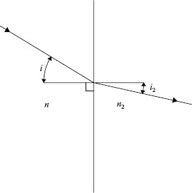
FIGURE 2.1 Refraction at a surface, Snell’s law.
Equation 2.1, when generalized into three dimensions, is the basis of all ray tracing and as might be expected, an expression in terms of the sines of angles in three dimensions leads to very little insight as to what is happening in the design. For that we need a simplification. We need the paraxial approximation.
If the ray is considered to be so close to the optical axis that its angles, and incidence heights are so small that the angles and their sines are proportional to their tangents, then we are in what is known as the paraxial region and many formulae can be simplified to much more interpretable paraxial forms. Snell’s law, for example, can be represented as in the following equation:
Paraxial approximations are potentially very useful. To use them, the angles need not actually be small, provided we remember that if they are not small then this is truly an approximation and the results cannot be relied upon for total accuracy. However, formulae based on this approximation will generally give a good prediction of where the focal planes will be, of image dimensions, and of approximately how large the lens apertures will need to be.
The paraxial approximation does give an accurate computation of the primary aberrations. Even better, for each of the seven primary aberrations, the total for the whole lens is the sum of individual surface contributions. The paraxial approximation permits these individual surface contributions to be calculated, enabling the designer to see where in the system problems are arising.
If in addition we assume that not only is the paraxial approximation true but also that the lenses have zero center thickness, then this is known as the thin lens approximation. The height of the paraxial ray is the same at both surfaces of a lens element and further simplifications result. Systems can be sketched as a series of simple line objects as shown in Figure 2.2, where we see two lenses of power k (the power k is the reciprocal of the focal length, and they are subscripted 1 and 2). The lenses are separated by a distance d1. A ray is incident at a height h1 and at an angle u1 at the first lens where it is refracted and leaves lens 1 at an angle u2. The path of the ray through lens 1 arriving at lens 2 at a height h2 can be calculated using the following simple formulae:
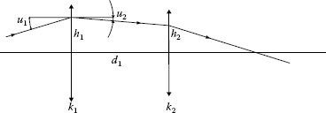
FIGURE 2.2 Refraction of a ray at a thin lens.
The notation is Cartesian. A good account of this theory and that of paraxial aberrations, paraxial theory, and the Seidel aberrations may be found in Welford [3].
The thin lens layout is an ideal point in the synthesis of the design for the designes to confirm that they have provided sufficient space for fold mirrors and prisms, that any windows or filters will not be uneconomically large, and a variety of other fundamental considerations.
In principle, the five monochromatic primary aberration totals for the whole lens describing its performance over the whole field and for all apertures. The mix of aberrations at a particular point of the field of view, and for a given F/number of the lens will result from the power series variables in aperture and field.
The designer only needs to minimize the five aberration totals, and then all variants of aperture and field of view should be corrected. Just five numbers describe the whole monochromatic lens performance. It is this remarkable simplification that permits designers to understand even complex systems.
In reality, higher-order aberrations may well become important at large field angles and apertures, but if the designer has the five primary aberrations under control, they can fairly and safely leave the optimization program to attempt to correct the higher orders.
The five aberrations are spherical aberration, coma, astigmatism, field curvature, and distortion. Although they are all of fourth order (in aperture and field), the extent to which the fourth order consists of aperture terms or field terms changes as we go through the list.
Spherical aberration is independent of field, and is constant over the whole field. By contrast, distortion is independent of aperture, so it does not matter whether the lens is used at F/1 or F/32, the distortion will not change. Coma is less dependent on aperture but is linearly dependent on field. Astigmatism and field curvature are dependent on the square of aperture (being essentially defocus in effect) and on the square of field angle.
For an image of a very small star-like source, spherical aberration is the only aberration that can occur on axis, it appears as a symmetrical circular blur of light. Depending on the sign of the aberration total, it will be a small disk on one side of focus and a small bright ring on the other.
Coma manifests as a small comet tail. The nominal image point is at the point of the comet tail. The tail gets wider as it grows away from the nominal image point. These wider regions are light that came from the outer zones of the lens aperture, so that if the lens is closed down from say F/1 to F/4, the coma seen will greatly reduce. The point of the tail remains fixed but the extent of the tail decreases.
As has been mentioned, the primary aberrations are the only series terms that have the correct symmetry properties, so that if the small comet tail points upward in the upper half of the scene then it points downward in the lower half, maintaining symmetry. Any term that would not have done this would have been excluded from the power series. Thus the coma term is linear in field so that it changes symmetrically across the optical axis.
Astigmatism and field curvature are often grouped as a pair because their origins and consequences intertwine.
Consider a test chart consisting of radial lines and concentric circles. If astigmatism is present and there is no field curvature, then as we move out across the field we find increasingly that we can either focus the radial lines or we can focus concentric circles, but we cannot get both to focus at the same time. One astigmatic focus will be nearer to the lens, and the other slightly further away relative to the nominal focal plane. Which way around these are dependent on the sign of the astigmatism total.
Now consider the same chart for a lens that has zero astigmatism but a nonzero field curvature total. Now as we progress across the field, we find that we can focus both circles and radial lines at the same time, but as we move outward across the field, the place of common focus moves away from the nominal focal plane. A focal surface of good imagery exists, but it is either concave or convex. That is, there is a field curvature. Whether the surface is convex or concave depends on the sign of the field curvature aberration total for the lens. Now we shall see why these two terms are often combined.
Consider a lens in which the astigmatism and field curvature totals are both nonzero. In this case, we find two curved focal surfaces of different curvatures. On one curved focal surface, the radial lines are in focus, and on the other the concentric circles are in focus. It is useful to note that if we cannot correct astigmatism or field curvature fully, we may introduce the other in just sufficient quantity to cause the surfaces to be equally concave and convex. That is, the two surfaces depart from the flat nominal focal plane, symmetrically, one in front of the plane and the other behind it. This compromise generally gives the best result when either astigmatism or field curvature cannot be fully corrected. Field curvature is also commonly known as Petzval curvature or Petzval sum.
Distortion is a variation of magnification with field angle. If we double the field angle, then the distance of the image from the optical axis, across the focal surface, should also approximately double. The effect of distortion is to cause the image to be further (or less) from the center of the image plane than it should be. The effect of distortion increases as the field angle increases. It may be unnoticeable for small field angles but become very pronounced at the edge of the field. The effect is not necessarily small and may be very intrusive. Zoom lenses for news gathering often have large amounts of distortion and can create a characteristic seasickness effect as the camera is swept across the scene, the motion of the scene increases as it reaches the edge of the field of view. It is such a large effect that a television zoom lens was once marketed as ×13 because inward distortion at narrow angle combined with outward distortion at wide angle to give ×13 change of field angle, even though the change in focal length was only ×10.
The above description of the primary monochromatic aberrations is intended to give the reader a feel for what is meant by the terms used by designers. There are many textbooks, such as those by Welford [3] and Born and Wolf [4] that the reader can refer to for a more mathematical account. Unfortunately the subject is one where the mathematics tends to obscure rather than illumine. This short chapter cannot cover the subject adequately. There are very few good texts on practical optical design. Laikin [1] is excellent as is Kingslake [2] although Kingslake’s notation is archaic. The conventional routes into the subject are either the small number of master degree courses (Imperial, London and University of Arizona typically) or to be taught on the job by an experienced designer.
A small number of engineers find it an interesting challenge to teach themselves and I admire them, but am grateful to Charles Wynne and Gordon Cook who taught me!
2.8 THIN LENS SEIDEL ABERRATION FORMULAE
Formulae exist, derived by Wynne [3,5], from which the primary aberrations of a thin lens system can be calculated, based on glass types and basic constructional data. They were derived by Wynne [5] nearly a century after Seidel derived the surface-by-surface formulae. Optical design is not a subject that changes quickly.
In these equations, the radii of curvature of each lens become a single variable known as the shape or bend of the lens. The resulting sets of biquadratic equations in the bend describe the available solutions. Solving large sets of simultaneous biquadratic equations does not lead to clarity of understanding. In fact, analytical solution of the equations is impractical for systems more complex than a doublet. A triplet can be solved, but requires an iteration to choose the glass type for the middle lens. It lies beyond the scope of this chapter but the author has found that this form of theory is much more useful when studying aspheric lens systems. Because the equation sets are simpler (those for the aspheric terms are linear rather than quadratic), generic equations that describe whole families of useful designs can be derived.
The equations for individual lens elements do describe the way in which the aberration totals for that element will vary with shape, depending on whether they are before or after the stop of the system. Novice designers can program these and will find them helpful. Later, they will not need to actually use the formulae explicitly, because knowing what they would predict in general terms is sufficient.
The fundamental design variable in these formulae is the shape or bend of the lens. If a lens has surface radii of curvature r1 and r2 then (where c = 1/r) the shape or bend B is given by
Figure 2.3 shows the cross section of a lens altering with bend (it also illustrates why designers refer to the process as bending a lens element).
Frequently, the aberration totals for an optical element are quadratic in bend. That is, they are represented by a parabolic curve. This means that there are different bends at which each aberration has an extremum (a maximum or minimum as the case may be) and these extrema cannot be exceeded. Very often, zero does not lie within the scope of the parabola. So that, for example, the spherical aberration of a single element lens cannot generally be set to zero by choosing its bend. To achieve zero, either one surface must become aspheric or a positive lens must be paired with a negative lens, and their shapes chosen so that the negative contribution of one cancels the positive contribution of the other, and so the path to system complexity begins.
Although laying out a complex system (consisting of separated groups of simple lenses) as a series of thin lenses (each representing a complete group, see, e.g., Figures 2.15 and 2.16 later in the chapter) can be helped by paraxial and thin lens formulae, it is still too great an approximation to assist in laying out a complex lens such as a microscope objective or camera lens.
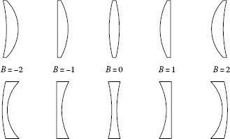
FIGURE 2.3 Shape or bend B of a lens element.
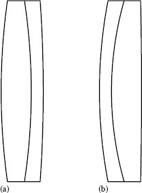
FIGURE 2.4 (a) Fraunhofer and (b) Steinheil doublets.
This degree of simplification neither will predict the resolution of the system nor will it cope accurately with ray paths at large angles to the axis. However, it will always be true that if the paraxial ray paths in a thin lens layout predict excessively large angles and apertures, then the design problems that will result will be nontrivial and other layouts should be considered before proceeding.
The calculation of the Seidel aberrations, the lowest terms of the polynomial that describes the wave-front as it exits the lenses, is provided within all well-known optical design programs. It shows very reliably the surfaces creating largest problems, helping greatly with the process of altering the structure in search of a better starting point.
We have said that we cannot rely on the program to correct a poorly chosen starting point. A simple example may be sufficient to demonstrate the problem. The dispersion is a measure of the rate of variation of refractive index with wavelength, the Abbe number, see below.
Figure 2.4 shows two lenses of identical focal length and aperture. In one lens, the high-index high-dispersion element (the negative component) leads, and in the other it comes second. These are both achromatic doublets and in both the two most important aberrations (spherical aberration and coma) have been corrected. Whether the negative lens first (the Steinheil doublet) or the negative lens second (the Fraunhofer doublet) is the better solution depends on many factors, sometimes one is better, sometimes the other.
The important thing to appreciate is that once one lens or the other has become the starting point, the optimization program is unable to reach the other solution. To do so it would need to reverse the glass types and there is no way to do so without passing through a situation where either the refractive indices or dispersions are equal. Optimization programs are constrained to choose paths along which designs get better, rather than ones that get worse and then get better.
So, if in this simplest of cases we cannot get from even a reasonably well-chosen starting point to a better one, then it is equally likely that a more complex system will have little chance of overcoming a fundamentally badly chosen starting point, but we shall have much less chance of guessing why.
It is the designer who must make manual drastic changes to the basic design structures. If glass types need reversing, or lens elements need to be added, then that must be done manually as a result of insight on the part of the designer. Hammer and Global optimization routines that use random number strategies to attempt to locate better solutions exist, but may be better left until a designer has no idea what to do next.
A lens may be as simple as a magnifying glass, or as complex as a zoom lens containing 20 or more individual lenses. The individual lens components are more properly referred to as lens elements, and may be thick or thin, and formed of plastic, glass, or crystal. Their surfaces may be plano (flat), spherical, or nonspherical (aspheric). In GRIN materials, the refractive index varies radially. Finally, the lens may not actually be present but may have its effect resulting from a hologram.
In an introductory chapter such as this, we cannot cover all of these possibilities. By the time the more esoteric options are needed, the reader will inevitably be in contact with specialist suppliers and will have access to all the information and advice that they need.
The materials that can be used for lenses and prisms are determined by the wavelength to be used. Lenses and prisms for the infrared and ultraviolet are generally made from crystals, the choice is limited, and data for them are tabulated in the design programs. For the visible waveband, they utilize the optical glasses that have been developed specifically for the purpose. It has been known for centuries that adding lead oxide to the recipe for a glass, produces a much denser glass that has a higher refractive index and a greater dispersion. The dispersion of a glass is the rate at which its refractive index changes with wavelength, and is important because it determines the element’s contribution to chromatic aberration. Similarly, when used in a prism it is the dispersion that causes the well-known prismatic effect, the rainbow spectrum that was first explained by Isaac Newton.
There is an advantage in using a slightly higher refractive index in total-internal-reflection (TIR) prisms, because the higher index increases the range of angles at which TIR can occur. Increasing the index of the glass is generally a limited option because the higher index glasses are more expensive and the pieces required for prisms are quite large.
Higher index glasses are generally less expensive if the designer can accept that the dispersion increases. Glass suppliers provide charts showing their selection of glass types, plotted against refractive index n and dispersion (the Abbe number V that decreases as the dispersion increases) as shown in Figure 2.5. The glasses shown are those of the Japanese company Hoya. The chart illustrates the effort required to create the glasses at the top left of the chart. The natural line for glasses to follow is that of the right-hand boundary. This boundary line results from gradually adding more and more lead oxide to a basically window-glass recipe. To extend types to the upper left of the chart requires exotic additives such as Lanthanum, resulting in the expensive glass types that optical designers prize.
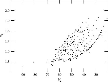
FIGURE 2.5 n−V glass chart.
To create such a plot, it is first necessary to choose three wavelengths, the first refractive index n1 is in the middle of the waveband of interest and two more are representative of the waveband at shorter and longer wavelengths. Glass manufacturers conventionally use the spectral d or e lines for the first wavelength. However, if designing for the near infrared or the ultraviolet you will need to recalculate (and perhaps replot) the n and V values because changes of waveband can change the relationships between glasses quite dramatically.
The Abbe number V is defined by numbering the wavelengths referred to as 1, 2, and 3, then,
In lenses too, a higher refractive index is often useful. In most cases, the contribution that a lens element (or surface) makes to the total aberration reduces as the index (and cost) increases. The automatic optimization program tends to increase the index if it can. To avoid increasing the chromatic aberration, the program may also alter the glass type to have both a high index and a low dispersion, increasing the material cost.
Most design programs permit the designer to set boundaries to the types of glass that it may choose, and it is possible to manually block the use of specific glasses. Glass suppliers can provide a list of guide prices, normalized relative to the classic crown glass 517642. This list should be at your right hand. It can be very difficult to revert to cheaper glass types later.
While discussing glass types, it is worth noting that it is wise for the lens designer to have good relations with the glass supplier’s local agent. The availability of glass types varies with time. Glass is made in batches depending on demand, and it is quite a commonplace for even a common glass type to be in worldwide shortage. Glass types may also be discontinued, without notice and for no apparently good reason. However, that glass type may be in sufficient stock worldwide that its termination will not have any effect for a long time. The supplier’s agent is your best source of information on all such matters.
Moldings are often cheaper than sawn block, because sawn block involves wastage and additional shaping processes at First-World labor rates. Molding allows the glass supplier to minimize waste, and may be carried out cheaply by a Third-World company.
Finally, beware of equivalents. Many glass types are intended to be equivalents such that one supplier’s glass can be used in place of another’s. This equivalence is often only partially true. Two glasses may have the same refractive index ne and the same V value. However, a detailed check may reveal that the partial dispersion, thermal expansion, density, chemical durability, or spectral-transmission curve may be different. This is even true for a specific supplier if they have changed the recipe of the glass, for example, while attempting to reduce the lead content.
There is a great advantage in being able to visit your usual lens supplier to discuss glass types, coating options, and details of the design (such as the edge thickness and the ratio of diameter to lens thickness). This is not necessarily the cheapest way to procure lenses but it is certainly a way to avoid expensive misunderstandings. The cheapest way is to cooperate with Far Eastern suppliers, such as those in the hi-tech zones in China. Careful choice of contact can result in very good prices for lenses in bulk. However, these suppliers frequently require a large minimum order, almost always 20 pieces and often a 100 piece minimum order.
This is suitable for production quantities, but creates the problem of where to buy the small quantities needed for the prototype. Bearing in mind that a prototype is supposed to represent the final product, to build the prototype with components that are not made by the production supplier is risky for two reasons. The first is that new problems at the production stage can turn that into a 100 item prototype batch. The second is more complex and will be covered shortly—the subject of stock tooling.
Experience suggests that if the designer is confident that the design will proceed to production then it may be better to accept the minimum order quantity for the prototype rather than build the prototype with one supplier and then start full-scale production with an as yet untested new supplier. However, if the system has high performance and contains extreme or expensive components, it may be better to forego low prices in favor of a local supplier with easier communication and a smaller minimum batch.
Traditionally, optical polishers use small lens-like glass tools to test components while still in place on the polishing machine [6]. These tools are polished plano on one side and on the other is a very precisely created optical surface. By placing it on the work piece, Newton’s rings reveal the difference between the work surface and the test-tool surface. The tools are polished in convex–concave pairs until they are near-perfect spheres (to λ/20 or so). Any departure from perfection when used on a work piece is then seen to be the current error in the work surface and the polisher uses this information to create a better surface (or figure), a process known as figuring.
In creating these highly precise tools, a great deal of skill is required to arrive at perfection at the same moment as the radius of curvature is the exact value requested by the designer. They are expensive to make and become part of the company’s assets. Optical designers are encouraged to use existing stock tools wherever possible.
Optical companies publish their lists of tools, frequently as datasets within ZEMAX, CODE-V, etc. Designers adjust their final design to suit their chosen supplier’s stock-tool list.
This then is the second reason why using different suppliers at the prototype and production stages creates problems. The designer has to fit a new set of stock tools, and the new design may be sufficiently different to require requalifying or the alteration of metal components.
The severity of the problem is also dependent on the sophistication with which the two suppliers are able to calibrate the radii of curvature. Interferometric measurement enables the radii to be known to almost micron precision, certainly better accuracy than the designer requires. Smaller polishing shops may still depend on an older technique, spherometry. In spherometry, a micrometer is used to measure the camber (height) of the surface over a known diameter.
A simple but ill-conditioned equation then allows the radius to be determined. The resulting radii are not known to be much better than 0.01% in the best circumstances and may well be in error by 1%.
In modern practice, both in the West and the Far East, surface testing can be done by interferometry. The radius is dialed into the instrument with an accuracy much better than spherometry. The figure is then tested relative to the designer’s data radius. In general, however, it is still more convenient and cheaper for glass tools to be used, and the designer is still encouraged to use stock radii. One or two surfaces with difficult stock tool problems may be left for interferometric testing.
Unusually in engineering practice, the designer will generally specify a radius of curvature with no tolerance assigned to it. By doing so, they are specifying not just a radius but a specific tool set.
The designer will of course need to assign tolerances for all other dimensions. We might expect the errors in manufacture to have a normal distribution, that is, a bell-shaped error curve centered on the nominal value. That would misunderstand the nature of the role of tolerances and dimensional errors in the traditional lens-making process.
Optical craftsmen work to accuracies that are much better than those on the drawings. The larger tolerances on the drawing are not there because the process is imprecise, they are there for a completely different reason—to reduce scrap.
For example, a thickness may be specified as 10.1–9.9 mm. What then is the most likely value if a batch is measured? A production engineer would say 10.0. In fact, the glass polisher is working to personal tolerances of tens of micrometers. They know that glass is prone to scratching and that if scratched at the moment that the batch of components is finished, the scrap item will need to be put aside, to become part of a rework batch, all of which will be slightly thinner than those that came out of the first round. There may even be a second rework batch that are even thinner.
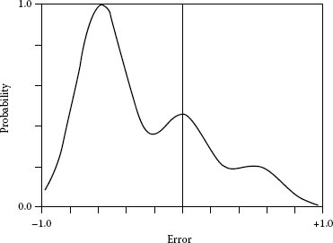
FIGURE 2.6 Distribution of yield within optical tolerance limits.
The polisher therefore aims for the first attempt to get a thickness just under the top limit, the second attempt to be around the mean dimension, and the third attempt to be just inside the lower limit.
The distribution is thus, not a bell-shaped normal distribution centered on the mean but a stepped distribution with the greatest number just under the top limit, see Figure 2.6. A designer who trusts the supplier to supply mainly first-attempt items may decide to bias the tolerances so that the upper limit is nearer to the actual value required. The lower limit is then lower than the value that can really be accepted, but is unlikely to occur. The designer accepts that there will be occasional unacceptable systems that need rectification, but the component cost will be kept down overall, and better systems will result because each component is on average better than if unbiased tolerances were used. This strategy works well when companies are polishing for their own products, but requires unusual rapport between workshop and designer. It does not work well if the purchaser or seller has adopted an aggressive strategy.
Rubbing two surfaces together randomly produces spherical surfaces by a process that has not changed significantly in seven centuries. To create a nonspherical (aspheric) surface requires much more dexterity in polishing or expensive machine tools. The use of aspheric surfaces can significantly reduce the number of components in a lens system [7,8,9], and their use should be seriously considered when the optical material is expensive, or expensive mold tools need to be made. Molded aspheric surfaces in glass and plastic have been used in millions in a DVD player. They are also used in glass optics to control higher-order aberration and distortion in expensive photographic and television objectives, provided they are manufactured in sufficient quantity for economies of scale to reduce the tooling costs to an acceptable level. They are common in cheap plastic optics because they reduce the number of mold tools required. Aspheric-surface costs do not matter so much for molds because even spherical surfaces may need aspheric mold surfaces, to allow for differential shrinkage.
2.14 TESTING AND SINGLE-WAVELENGTH SYSTEMS
Lens systems tend to be specified in terms of resolution. The equipment required to make this measurement is often built around commonly available lasers such as the HeNe 632.8 nm. A problem then arises when designing a system that only has a very good performance at the single wavelength of use, if the wavelength of use is a long way away from 632.8 nm. This can make it difficult or impossible to test the system adequately with any of the equipment that the company already possesses. The method of testing should always be in the designer’s mind at an early stage. If it will be very difficult, expensive, or impossible to test the lens system then this is a serious consideration.
The simplest prisms disperse light into a spectrum or act as beam splitters. These are well known and will not be dealt further here. More importantly, prisms can displace or rotate the direction of light propagation. This may simply be for design convenience, or it may be to invert, revert, or rotate the orientation of an image.
An advantage of a prism (relative to a mirror) is that it can often reduce the volume occupied by the system. This is shown in Figure 2.7. Here, the requirement is to alter the direction of propagation by 45°. A mirror is seen to be large compared with an equivalent Schmidt prism. Not only are the prism surfaces smaller because reflections within the prism are at less oblique angles but also the light beam is folded, reducing the space required for the system.
Clean prisms have almost zero loss at their TIR faces, while rear surface mirrors suffer absorption losses caused by the metal–glass interface. Front-surface mirror-coatings have higher reflectivity but the cost is greater and the surfaces are much less durable.
Prisms are inevitably expensive, and this is partly because many surfaces are used at oblique angles. Surfaces that are aligned normal to the optical axis are cheaper to polish. The reason is that a small change in focus can correct the effects of the usual surface tolerance of 1.5 wavelengths of curvature error. The optical polisher, using glass contact tools then only needs to get to within 1.5 wavelengths of the correct form to be able to detect 0.25 wavelength of elliptical error, the part of the tolerance that affects resolution.
However, this is not true of an oblique surface. For example, the mirror shown in Figure 2.7 is at 67.5° so the circular beam has an elliptical footprint on the surface, the major axis being 2.6 times the minor axis of the ellipse. Thus to a first order, a spherical form error of 1.5λ across the major axis would be decreased by a factor of 6.8 (i.e., 2.62) to 0.22λ across the minor axis. As a result, after reflection, one section of the beam has 6.8 times less wave-front error than the other section. The resulting astigmatism cannot be corrected by refocusing. A much tighter surface-figure tolerance should be specified for an oblique surface, with a consequent increase in cost.
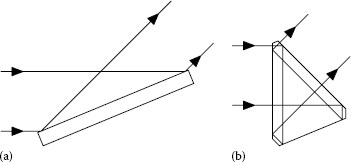
FIGURE 2.7 Comparison of (a) mirror and (b) Schmidt prism.
Introducing a prism into the light path affects the design of the rest of the system. When light is focused through a prism, such as a prism in the back-focal space of a lens, the prism will introduce; chromatic aberration, spherical aberration, coma, and astigmatism, and these need to be allowed for in the design of the lens itself.
Despite their cost, prisms have a vital role to play in correctly orientating the beams, in ways that can be difficult to reproduce using only lenses. We therefore need to understand how prisms operate, and also how to interpret what they are doing in our system.
If the deviation of light in a right-angle prism is in a horizontal plane then the image, just as with a mirror, remains upright but is reverted side to side. This is intuitively correct because the right-angle prism is just a mirror with glass in front of it.
But, how can we determine the image orientation in a more complex prism system? The right-angle prism is a good place to start. Many texts show prisms with a letter F entering and exiting a prism, thereby defining the beam orientation on exit for that prism type.
It is important to note that the direction in which the F is viewed is important. Both pictures in Figure 2.8 are correct. However, they appear to contradict. The problem is that Figure 2.8a is oriented so that the left-hand (entry) F is shown from behind while the right-hand (exit) F is shown in front. In Figure 2.8b, a more suitable orientation of the prism shows both the Fs from the direction in which they are propagating and the side-to-side reversion that would be expected is now seen. Extending this technique to a drawing of a more complex prism can be difficult.
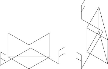
FIGURE 2.8 Image orientation in a right-angle prism.
An alternative simple way to determine the orientation of an image uses no more than a long narrow strip of paper that has a line drawn down one edge. Lay the paper strip on a drawing of the prism, and at each prism surface fold the paper along the reflection surface of the prism. The new direction of the strip at each fold is the direction of the beam after reflection. Eventually, at the point where the strip exits the prism, the position of the line along the edge of the paper defines whether or not the image has inverted. The technique is shown in use for the right-angle prism in Figure 2.9.
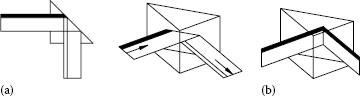
FIGURE 2.9 Folded paper-strip technique.
If the side-to-side reversion has been determined by the first folding, then any top–bottom inversion of the image can be interpreted from a second folding as shown in Figure 2.9b. From these, it is clear that the image has not inverted vertically but has only reverted horizontally. This technique requires practice and a little dexterity but is very useful for interpreting practical systems.
If the beam is actually focusing toward an image plane, with perhaps intermediate images within the train of prisms, then it may be necessary to create a scale print of the straightened optical system (i.e., with reflections removed but suitable blocks of glass to represent the presence of the prism in the system). The printout can be folded, as above, leading to a clear understanding of how the prisms interact with the optical system.
Ultimately, a fully three-dimensional nonsequential ray-trace can be set up, which will create enormous amounts of information about the passage of light through the prisms. The reader is cautioned, however, that enormous amounts of information are best created after the designer understands their system.
Almost all pairs of binoculars contain four Porro prisms. They create the familiar cranked shape. This common prism illustrates key design techniques.
A simple telescope (i.e., just an objective lens and an eyepiece) creates an image that is inverted vertically and reverted horizontally, the image has been rotated by 180°. The telescope becomes even longer if a relay stage is added to correct the orientation of the final image. During the Napoleonic wars, ship’s telescopes were known as “bring-‘em nears” and the image was in fact inverted.
Using Porro prisms to rotate the image has the additional benefit of folding the system to make it more compact. The Porro prism, shown in Figure 2.10a is simply a right-angle prism in which the light enters normal to the hypotenuse surface, is totally internally reflected at the two smaller faces, and exits via the hypotenuse surface. The Porro prism is shown in detail in Figure 2.10b. The paper-strip diagram in Figure 2.10a shows that in passing through a Porro prism whose long axis is vertical, the image has inverted. An image that required both inversion and reversion would now only require reversion. Conveniently, the light is now traveling away from the eyepiece. Therefore, a second Porro prism is placed with its long axis horizontal (Figure 2.10c), the image is reverted and when seen by the eyepiece, the scene has been rotated right way up and right way round, and the light is also traveling toward the eyepiece. The Porro-prism pair has folded the telescope into the familiar binocular shape, a much more convenient shape for use.
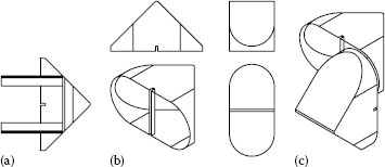
FIGURE 2.10 Porro prism.
Unlike the right-angle prism, that conventionally has square apertures, the Porro prism normally has hemi-cylindrically shaped ends, as seen in Figure 2.10b. This feature has a number of useful functions. Firstly, the removal of the glass reduces weight and volume. Secondly, the rounded ends are much more robust in an instrument that is frequently dropped. Thirdly, it is also easier to machine the housing to have rounded sockets to suit the ends of a Porro prism than it is to make a socket for a square prism. The difference may be small, but over hundreds of thousands of items the small savings add up, and it can be molded.
There is a chamfer along the line where the two small faces intersect. This protects the corner from chipping and provides a stronger edge across which to place a sprung metal strip to hold the prism in place. Commonly, the prisms are initially held just by the metal strips. Then they are adjusted until both arms of the binocular are looking in exactly the same direction. Finally, the prisms are secured in place with spots of glue.
Thus, the shape of the prism has been determined by a strong, convenient, and cheap method of assembly and adjustment.
The Porro prism has a slot, cut across the center of the hypotenuse face, apparently dividing the hypotenuse into an entry face and an exit face. In fact, it is doing rather more than that, but to understand and analyze its function, it is helpful to review another useful technique available to the designer—the tunnel diagram.
Figure 2.11a shows a general ray propagating through a Porro prism. However, if we were to look in through the entry face we would not see fold after fold, instead, we would see an apparently unfolded space, looking toward an exit face beyond which is the outside world (Figure 2.11b).
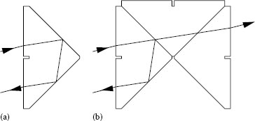
FIGURE 2.11 Porro prism tunnel diagram.
The designer initially determines the total glass path within the prism, and enters it in the optical design program as a simple block of glass, that fully represents the prism, as it relates to resolution, aberrations, etc.
However, to understand the relationship between the light beams and the physical features of the prism we need to do the opposite of the paper-strip technique. That is, instead of folding paper to represent light’s folded path through the prism, we may instead unfold the prism, so that light appears to pass through each reflection surface into another piece of glass. Just as with the paper strip, the reflection surface acts as a fold line and the shape of the next glass space within the prism (or at least a mirror image of it) is created, as what is known as a tunnel diagram (Figure 2.11b).
Let us use Figure 2.11b to consider the complex shape that has been developed. On viewing through the entry face, a glass–air interface is seen to one side, parallel to the line of sight, and on the other side two triangular glass spaces, each of which has a number of alternative and potentially incorrect exits from the prism, are seen. Various features also exist, created by the chamfers that are cut into the prism. This tunnel really does exist; it is not just an engineering fiction. If a Porro prism is available, the reader can immediately see that this really is what the prism looks like from the viewpoint of the light that is passing through it.
The tunnel diagram is useful for checking the relationship between the margins of the beam and the chamfers. The chamfers not only need to be far enough out from the beam to allow it to pass but also need to be far enough in to cut off access to the triangular side spaces through which light could pass creating ghost images. In particular, this diagram explains the slot across the middle of the hypotenuse face.
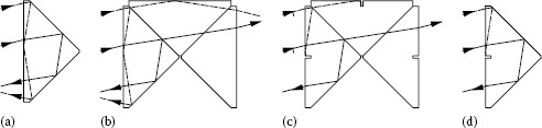
FIGURE 2.12 Ghost path within the Porro prism.
Figure 2.12a shows a Porro prism that has no slot, and we see that if a ray enters too close to the outer edge of the aperture, it can reflect at grazing incidence on the inside of the hypotenuse face, only after that does it reach the other small surface to reflect and exit through the hypotenuse exit face, but traveling at an angle to its correct path and creating a false or ghost image. These paths could be constructed on the drawing of a single prism, with many reflections to be constructed to gain a full understanding of which rays can follow this false path.
However, if we use the tunnel diagram (Figure 2.12b) it is easy to determine the rays that can reach the hypotenuse surface to follow the false path. There are no complex reflections to construct because light follows a simple path within the tunnel. It immediately becomes clear that the slot is a baffle to trap the false path at the point where it reaches the hypotenuse surface (Figure 2.12c and d). The slot can be drawn on the tunnel diagram to trap as much of the false path as necessary, while ensuring that the slot does not obstruct the straight-through correct path.
In principle, the tunnel diagram can be reduced in length so that its length is equal to the equivalent path in air. This allows the designer to ignore refraction at the entry and exit faces. This sounds convenient. However, any serious optical design requires that the aberrations due to the presence of the glass be taken into account in the design of the associated lenses. The reduced tunnel is also much more complicated to draw. The author has always found the glass tunnel to be much more useful than the reduced tunnel. The folded-strip technique and the tunnel diagram between them solve most of the problems involved in obtaining a working understanding of a prism system. The concepts can be extended to the folding of complete optical systems using large-scale prints from the optical design program.
Modern binoculars use a variety of straight-through prisms to create small compact systems. An early version of this type of prism is the Pechan. It is shown in Figure 2.13, together with its paper-strip diagram. It has a diagonal airspace just thick enough to support TIR. It can be seen that a very large amount of a system’s length can be folded into this compact prism, leading to very small systems, which is why many World War I officers carried these as vest-pocket binoculars.
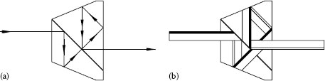
FIGURE 2.13 Pechan prism.
Figure 2.14 shows the Abbe prism. It serves a similar function, and shows how two prisms having the same function can create very different profiles for a system.
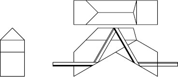
FIGURE 2.14 Abbe prism.
Simply creating an image with the correct focal length optics is sometimes not enough to create the ideal system. This is particularly true of lenses that relay image planes. It is also true of those that measure size. In both cases, the designer can significantly improves the system by adding a little sophistication to the layout.
Figure 2.15a shows a series of relay lenses. Clearly, as the light is relayed, less of it is caught by the second lens. Simply relaying the image plane was not sufficient. In Figure 2.15b we see a system in which an extra lens at the intermediate image plane relays the image of the lens aperture. That is, we now have two interleaved relay systems, one relaying the image and the other relaying the lens aperture. It requires no further explanation to appreciate the advantage of adding the second set of lenses. A lens placed at an image plane to relay the aperture is known as a field lens. Incidentally, the surfaces of a field lens should not be quite in the image plane, because any scratches or dust will be in focus and will be added to the scene. The lens should therefore be close to, but not actually at, the image plane.
Optical catalogs contain telecentric lenses for measuring systems. Telecentricity is important, both of itself and also as an example of how a measuring system can be improved by insight into how it operates. Telecentric lenses are almost always much larger than a simple camera lens of the same focal length. Often, they are also of much larger F/number. A camera lens may be F/1.4 but F/4 is quite a good aperture for a telecentric lens. They are more expensive, so a designer may well opt for the cheap lens with the bigger signal. Such a simplistic choice is shown as a thin lens layout in Figure 2.16a.
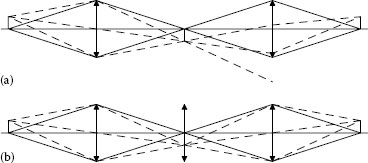
FIGURE 2.15 Relay systems.
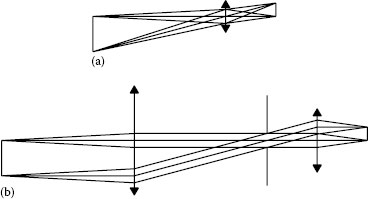
FIGURE 2.16 Telecentric lenses.
Here we see a simple lens (perhaps a doublet or a cheap camera lens). It is imaging an object with a magnification of −0.5. The designer hopes that they have a perfect system for measuring the object by determining its size on a camera chip. Measuring a reference object and correcting for any distortion, the test object may be measured to a few tens of microns—if it is in focus!
From Figure 2.16a we see that if the object were slightly too near the camera it would appear slightly larger, and if the camera chip were slightly too near the lens, the object would appear slightly too small. Of course, in both cases the image would be blurred by defocus, but from a measurement point of view it is the error in size that is more important. Figure 2.16b shows a much more complex system in which the light from the object to the lens and from the lens to the camera chip both travel substantially parallel to the axis of the instrument. As a result, an out-of-focus image will be blurred but it will not have changed in size, calibration will be correct, and only the resolution would have been degraded.
Photogrammetry lenses for aerial survey normally have the film held by vacuum against a glass plate, to define the film’s position accurately. If the vacuum is imperfect the film may be slightly rumpled. That is why all good photogrammetry lenses should have telecentric illumination at the film plane, so that images remain in the correct place. Telecentricity then is the condition in which light leaves an object or approaches the image with its chief (central) ray normal to the object or focal plane.
Incidentally, Figures 2.15 and 2.16 are good examples of the value of using thin lens layouts to think through the underlying problems of a system.
In addition to introducing the problems involved in designing an optical system, the opportunity has been taken to provide a practical toolbox of techniques, and things to consider when setting out to design an optical system. Other concepts such as the modulation transfer function and theoretical resolution limits, coherence and partial-coherence, etc., have been omitted. An introductory chapter could not have treated them with any degree of rigor, and it is hoped that the material presented instead is of more practical assistance.
REFERENCES
1. Laikin, M., Lens Design, Dekker, New York, 1990.
2. Kingslake, R., Lens Design Fundamentals, Academic Press, New York, 1978.
3. Welford, W.T., Aberrations of Optical Systems, Adam Hilger Ltd., London, U.K., 1986.
4. Born, M. and Wolf, E., Principles of Optics, 6th edn., Pergamon, London, U.K., 1993.
5. Wynne, C.G., Thin lens aberration theory, Optica Acta, 8(3), 255–265, 1961.
6. Horne, D.F., Optical Production, 2nd edn., Institute of Physics, London, U.K., 1982.
7. Hall, P.R., Use of aspheric surfaces in infra-red optical design, Optical Engineering, 26, 1102–1111, 1987.
8. Altman, R.M. and Lytle, J.D., Optical design techniques for polymer optics, International Lens Design Conference 1980, Proc. SPIE, 237, 380–385, 1980.
9. Kuttner, P., Optical systems with aspheric surfaces for the correction of spherical aberration as main error in the infra-red and visible spectral regions, Aspheric Optics, Design, Manufacture and Testing Conference, London, U.K., 1981, Proc. SPIE, 235, 7–17, 1981.