Chapter 13 Polarization

For all electromagnetic radiations, the oscillating components of the electric and magnetic fields are directed at right angle to each other and to the propagation direction. Because a magnetic field vector of the radiation is unambiguously determined by its electric field vector, the polarization analysis considers the last one only. Here, we shall use a right-handed Cartesian coordinate system XYZ, with the Z-axis pointing along the direction of propagation.

Let us assume that we have a plane harmonic wave of angular frequency ω, which is traveling with velocity c in the direction Z. The angular speed is ω = 2π(c/λ), where λ is the wavelength.

The electric field vector has two components E_x(z,t) and E_y(z,t), which can be written as

$\begin{array}{l} E_{x} (z, t) = E_{0 x} \cos [ω (t - \frac{z}{c}) + δ_{x}] \\ and \\ E_{y} (z, t) = E_{0 y} \cos [ω (t - \frac{z}{c}) + δ_{y}] \end{array}$ $\begin{array}{l} E_{x} (z, t) = E_{0 x} \cos [ω (t - \frac{z}{c}) + δ_{x}] \\ and \\ E_{y} (z, t) = E_{0 y} \cos [ω (t - \frac{z}{c}) + δ_{y}] \end{array}$

(13.1)

where

E_0x and E_0y are the wave amplitudes

δ_x and δ_y are arbitrary phases

t is the time

The phase differenc between two components can be denoted as δ = δ_y − δ_x, where 0 ≤ δ < 2π.

13.2 DEGENERATE POLARIZATION STATES

Particular cases of propagation of the two components given earlier are shown in Figure 13.1. The central part illustrates a distribution of electric field strength along the Z-axis at some moment of time t = 0. Phase of the y-component δ_y is zero and δ_x = −δ correspondingly. The axes E_x and E_y have units V/m. The unit length along Z-axis is one wavelength. The wave is moving forward, and the tip of the electric strength vector generates a Lissajous figure in the E_xE_y-plane. The shape traced out by the electric vector when such a plane wave passes over it is a description of the polarization state.

The right part in Figure 13.1 represents the corresponding loci of the tip of the oscillating electric field vector. The shown cases are called degenerate polarization states: (1) linearly horizontal polarized (LHP) light, E_0y = 0; (2) linearly vertical polarized (LVP) light, E_0x = 0; (3) linearly +45° polarized (L + 45P) light, E_0x = E_0y = E₀, δ = 0; (4) right circularly polarized (RCP) light, E_0x = E_0y = E₀, δ = π/2; (5) linearly −45° polarized (L − 45P) light, E_0x = E_0y = E₀, δ = π; and (6) left circularly polarized (LCP) light, E_0x = E_0y = E₀, δ = 3π/2. The RCP light rotates clockwise, and the LCP light rotates counterclockwise when propagating toward the observer.

The clockwise sense of the circle describing right circular polarization is consistent with the definition involving a right-handed helix: if a right-handed helix is moved bodily toward the observer (without rotation) through a fixed transverse reference plane, the point of intersection of helix and plane executes a clockwise circle. This classical convention of right and left polarizations is accepted by most authors [1,2,3,4].

However, some authors do not agree, and they use the opposite definition of polarization handedness [5,6,7]. The latter refers to the quantum-mechanical properties of light. In this description, a photon has an intrinsic (or spin) angular momentum of either negative −h/2π or positive h/2π, where h = 6.626 × 10⁻³⁴ J s is Planck’s constant. The angular momentum is parallel to the direction of the photon’s propagation. In the classical convention, the positive and negative momentums correspond to LCP and RCP photons, respectively. The alternative approach suggests to designate the positive momentum to the right polarized light. Here, we will follow the classical convention.

13.3 POLARIZATION ELLIPSE

In a general case, the Lissajous figure of two perpendicular sinusoidal oscillations with same frequencies and stable phase difference is an ellipse. Thus, both linear and circular polarized light may be considered as special cases of elliptically polarized light. In order to find an equation of the corresponding locus, we have to eliminate the time–space term ω(t − (z/c)) + δ_x in the system (13.1). Expand the expression for E_y(z,t) and combine it with E_x(z,t)/E_0x to yield

$\sin [ω (t - \frac{z}{c}) + δ_{x}] \sin δ = \frac{E_{x}}{E_{0 x}} \cos δ - \frac{E_{y}}{E_{0 y}} .$ $\sin [ω (t - \frac{z}{c}) + δ_{x}] \sin δ = \frac{E_{x}}{E_{0 x}} \cos δ - \frac{E_{y}}{E_{0 y}} .$

(13.2)

Then, we multiply both parts of expression (13.1) by sin δ

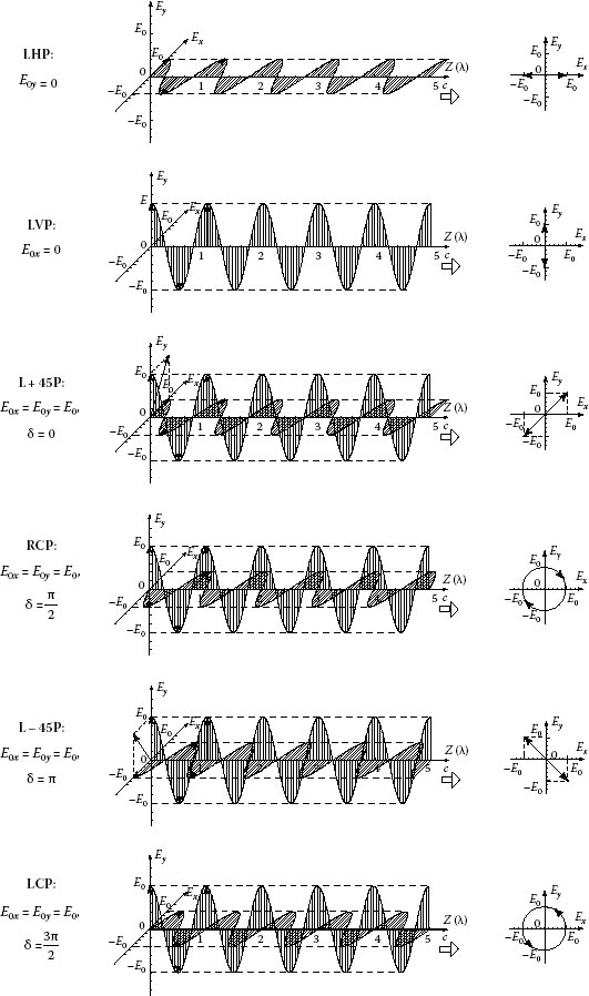
$\cos [ω (t - \frac{z}{c}) + δ_{x}] \sin δ = \frac{E_{x}}{E_{0 x}} \sin δ .$ $\cos [ω (t - \frac{z}{c}) + δ_{x}] \sin δ = \frac{E_{x}}{E_{0 x}} \sin δ .$

(13.3)

FIGURE 13.1 Degenerate polarization states.

Finally, by squaring and adding Equations 13.2 and 13.3, we have

${(\frac{E_{x}}{E_{0 x}})}^{2} + {(\frac{E_{y}}{E_{0 y}})}^{2} - 2 \frac{E_{x}}{E_{0 x}} \frac{E_{y}}{E_{0 y}} \cos δ = \sin^{2} δ .$ ${(\frac{E_{x}}{E_{0 x}})}^{2} + {(\frac{E_{y}}{E_{0 y}})}^{2} - 2 \frac{E_{x}}{E_{0 x}} \frac{E_{y}}{E_{0 y}} \cos δ = \sin^{2} δ .$

(13.4)

This formula describes an ellipse, which is called the polarization ellipse.

The standard form equation of an ellipse with semi-major axis a and semi-minor axis b is the following:

${(\frac{E_{x}^{'}}{a})}^{2} + {(\frac{E_{y}^{'}}{b})}^{2} = 1.$ ${(\frac{E_{x}^{'}}{a})}^{2} + {(\frac{E_{y}^{'}}{b})}^{2} = 1.$

(13.5)

Expression (13.5) can be transformed to the expression (13.4) by a coordinate rotation on angle ψ:

$\begin{array}{l} E_{x}^{'} = E_{x} \cos ψ + E_{y} \sin ψ, \\ E_{y}^{'} = - E_{x} \sin ψ + E_{y} \sin ψ . \end{array}$ $\begin{array}{l} E_{x}^{'} = E_{x} \cos ψ + E_{y} \sin ψ, \\ E_{y}^{'} = - E_{x} \sin ψ + E_{y} \sin ψ . \end{array}$

(13.6)

Thus, the equation of ellipse with the major axis at angle ψ becomes

$E_{x}^{2} (a^{2} \sin^{2} ψ + b^{2} \cos ψ) + E_{y}^{2} (a^{2} \cos^{2} ψ + b^{2} \sin ψ) + E_{x} E_{y} (b^{2} - a^{2}) \sin 2 ψ = a^{2} b^{2} .$ $E_{x}^{2} (a^{2} \sin^{2} ψ + b^{2} \cos ψ) + E_{y}^{2} (a^{2} \cos^{2} ψ + b^{2} \sin ψ) + E_{x} E_{y} (b^{2} - a^{2}) \sin 2 ψ = a^{2} b^{2} .$

(13.7)

The formula (13.5) can be written in a similar way:

$E_{x}^{2} E_{0 y}^{2} + E_{y}^{2} E_{0 x}^{2} - 2 E_{x} E_{y} E_{0 x} E_{0 y} \cos δ = E_{0 x}^{2} E_{0 y}^{2} \sin^{2} δ .$ $E_{x}^{2} E_{0 y}^{2} + E_{y}^{2} E_{0 x}^{2} - 2 E_{x} E_{y} E_{0 x} E_{0 y} \cos δ = E_{0 x}^{2} E_{0 y}^{2} \sin^{2} δ .$

(13.8)

Comparing coefficients in the quadratic equations (13.7) and (13.8) yields

$\begin{array}{l} E_{0 y}^{2} = a^{2} \sin^{2} ψ + b^{2} \cos^{2} ψ, \\ E_{0 x}^{2} = a^{2} \cos^{2} ψ + b^{2} \sin^{2} ψ, \\ 2 E_{0 x} E_{0 y} \cos δ = (a^{2} - b^{2}) \sin 2 ψ, \\ \pm E_{0 x} E_{0 y} \sin δ = a b . \end{array}$ $\begin{array}{l} E_{0 y}^{2} = a^{2} \sin^{2} ψ + b^{2} \cos^{2} ψ, \\ E_{0 x}^{2} = a^{2} \cos^{2} ψ + b^{2} \sin^{2} ψ, \\ 2 E_{0 x} E_{0 y} \cos δ = (a^{2} - b^{2}) \sin 2 ψ, \\ \pm E_{0 x} E_{0 y} \sin δ = a b . \end{array}$

(13.9)

Subtracting the first equation of system (13.9) from second, we obtain

$E_{0 x}^{2} - E_{0 y}^{2} = (a^{2} - b^{2}) \cos 2 ψ .$ $E_{0 x}^{2} - E_{0 y}^{2} = (a^{2} - b^{2}) \cos 2 ψ .$

(13.10)

The major axis orientation ψ of the polarization ellipse can be found after dividing the third equation in (13.9) by Equation 13.10:

$\tan 2 ψ = \frac{2 E_{0 x} E_{0 y}}{E_{0 x}^{2} - E_{0 y}^{2}} \cos δ .$ $\tan 2 ψ = \frac{2 E_{0 x} E_{0 y}}{E_{0 x}^{2} - E_{0 y}^{2}} \cos δ .$

(13.11)

The orientation is the angle between the major axis of the ellipse and the positive direction of the X-axis. All physically distinguishable orientations can be obtained by limiting ψ to the following range:

$- \frac{π}{2} \leq ψ < \frac{π}{2} .$ $- \frac{π}{2} \leq ψ < \frac{π}{2} .$

(13.12)

The shape of the polarization ellipse can be expressed by a number called the ellipticity of the ellipse, which is the ratio of the length of the semi-minor axis b to the length of its semi-major axis a:

$e = \frac{b}{a} .$ $e = \frac{b}{a} .$

(13.13)

Dividing the fourth equation of system (13.9) by the sum of first and second equations, we get

$\frac{e}{1 + e^{2}} = \pm \frac{E_{0 x} E_{0 y}}{E_{0 x}^{2} E_{0 y}^{2}} \sin δ .$ $\frac{e}{1 + e^{2}} = \pm \frac{E_{0 x} E_{0 y}}{E_{0 x}^{2} E_{0 y}^{2}} \sin δ .$

(13.14)

The definition of ellipticity in polarization optics incorporates also the handedness by allowing the ellipticity to assume positive and negative values, to correspond to right-handed and left-handed polarizations, respectively. Using this notation, it is easily seen that all physically distinguishable ellipticity values can be obtained by limiting e to the range

$- 1 \leq e \leq 1.$ $- 1 \leq e \leq 1.$

(13.15)

However, according to the classical convention of the polarization handedness, the sign of ellipticity is opposite to the sign of angular momentum of light.

It is convenient to use an ellipticity angle ε such that

$e = \tan ε .$ $e = \tan ε .$

(13.16)

From Equation 13.15, it follows that ε is limited to the range

$- \frac{π}{4} \leq ε \leq \frac{π}{4} .$ $- \frac{π}{4} \leq ε \leq \frac{π}{4} .$

(13.17)

Now from (13.14), we have

$\sin 2 ε = \frac{2 E_{0 x} E_{0 y}}{E_{0 x}^{2} + E_{0 y}^{2}} \sin δ .$ $\sin 2 ε = \frac{2 E_{0 x} E_{0 y}}{E_{0 x}^{2} + E_{0 y}^{2}} \sin δ .$

(13.18)

The two Equations 13.11 and 13.18 can be rewritten completely in trigonometric terms by introducing an auxiliary angle σ (0 ≤ σ ≤ π/2) such that

$\tan σ = \frac{E_{0 y}}{E_{0 x}} .$ $\tan σ = \frac{E_{0 y}}{E_{0 x}} .$

(13.19)

This leads to purely trigonometric equations:

${\begin{array}{l} \tan 2 ψ = \tan 2 σ \cos δ \\ \sin 2 ε = \sin 2 σ \sin δ \end{array} .$ ${\begin{array}{l} \tan 2 ψ = \tan 2 σ \cos δ \\ \sin 2 ε = \sin 2 σ \sin δ \end{array} .$

(13.20)

13.4 POLARIZATION ELLIPSE TRANSFORMATIONS

Formulas (13.20) allow to calculate the orientation and ellipticity angles ψ and ε if we know the ratio and the phase difference of two components tan σ and δ in particular coordinate system.

For example, both the components are either in-phase or antiphase δ = 0 or δ = π. Then, formulas (13.20) yield

${\begin{array}{l} ψ = σ \\ ε = 0 \end{array} if δ = 0 and {\begin{array}{l} ψ = - σ \\ ε = 0 \end{array} if δ = π .$ ${\begin{array}{l} ψ = σ \\ ε = 0 \end{array} if δ = 0 and {\begin{array}{l} ψ = - σ \\ ε = 0 \end{array} if δ = π .$

Thus, the light is linearly polarized at the orientation angle ψ determined by the component ratio, and the angle ψ is positive for the in-phase components and negative for the antiphase components.

Let us consider the second example when the phase difference equals to quarter or three quarter wave, δ = π/2 or δ = 3π/2. According to formulas (13.20), we obtain the following:

$for δ = \frac{π}{2} : {\begin{array}{l} ψ = 0 \\ ε = σ \end{array} if 0 \leq σ < \frac{π}{4}, {\begin{array}{l} ψ = \frac{π}{2} \\ ε = \frac{π}{2} - σ \end{array} if \frac{π}{4} < σ \leq \frac{π}{2}, and {\begin{array}{l} ψ is not defined \\ ε = \frac{π}{4} \end{array} if σ = \frac{π}{4} .$ $for δ = \frac{π}{2} : {\begin{array}{l} ψ = 0 \\ ε = σ \end{array} if 0 \leq σ < \frac{π}{4}, {\begin{array}{l} ψ = \frac{π}{2} \\ ε = \frac{π}{2} - σ \end{array} if \frac{π}{4} < σ \leq \frac{π}{2}, and {\begin{array}{l} ψ is not defined \\ ε = \frac{π}{4} \end{array} if σ = \frac{π}{4} .$

$for δ = \frac{3 π}{2} : {\begin{array}{l} ψ = 0 \\ ε = - σ \end{array} if 0 \leq σ < \frac{π}{4}, {\begin{array}{l} ψ = \frac{π}{2} \\ ε = σ - \frac{π}{2} \end{array} if \frac{π}{4} < σ \leq \frac{π}{2}, and {\begin{array}{l} ψ is not defined \\ ε = - \frac{π}{4} \end{array} if σ = \frac{π}{4} .$ $for δ = \frac{3 π}{2} : {\begin{array}{l} ψ = 0 \\ ε = - σ \end{array} if 0 \leq σ < \frac{π}{4}, {\begin{array}{l} ψ = \frac{π}{2} \\ ε = σ - \frac{π}{2} \end{array} if \frac{π}{4} < σ \leq \frac{π}{2}, and {\begin{array}{l} ψ is not defined \\ ε = - \frac{π}{4} \end{array} if σ = \frac{π}{4} .$

The light is elliptically polarized with the major axis oriented along to X- or Y-axis. The polarization is right handed if δ = π/2 and left handed if δ = 3π/2. If amplitudes of the components are equal (σ = π/4), the light is circularly polarized and does not have the major axis. In this case, the first Equation 13.20 contains product of infinity and zero that cannot be defined.

Systems (13.20) allow to solve the direct problem: to compute angles of polarization ellipse ψ and ε if parameters of polarization components σ and δ are known. It is important for practical application to have a solution of the inverse problem: to compute parameters of polarization components σ and δ in particular coordinate system if angles of polarization ellipse ψ and ε are known.

The inverse solution can be found by transformation of Equations 13.20:

${\begin{array}{l} \cos 2 σ = \cos 2 ε \cos 2 ψ \\ \tan δ = \tan 2 ε / \sin 2 ψ \end{array} .$ ${\begin{array}{l} \cos 2 σ = \cos 2 ε \cos 2 ψ \\ \tan δ = \tan 2 ε / \sin 2 ψ \end{array} .$

(13.21)

An example of polarization ellipse with corresponding angles is illustrated in Figure 13.2. Here, orientation angle ψ = 30°, ellipticity angle ε = 22.5° (b/a = 0.41), and the handedness is clockwise (right-handed polarization). Using formulas (13.21), we can compute ratio angle σ and phase difference δ in the XY-coordinate system: σ = 34.6° (E_0y/E_0x = 0.7) and δ = 49°.

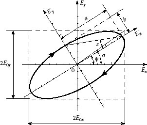
FIGURE 13.2 Polarization ellipse.

In the X′Y′-coordinate system, which is oriented along the major and minor axes, orientation angle is zero. The ellipticity angle ε does not change, and it equals 22.5°. The corresponding ratio angle σ′ and phase difference δ′ will be the following: $σ^{'} = {22.5}^{\circ} (E_{0 y}^{'} / E_{0 x}^{'} = 0.41)$ $σ^{'} = {22.5}^{\circ} (E_{0 y}^{'} / E_{0 x}^{'} = 0.41)$ and δ′ = 90°.

In the majority cases, we will not be interested in the absolute intensity of an optical wave. This justifies the use of a definition for the intensity of the wave that overlooks a constant multiplicative factor. Thus, we may express the intensity I simply as the squared amplitudes of the component oscillating along two mutually perpendicular directions:

$I \equiv E_{0 x}^{2} + E_{0 y}^{2} = a^{2} + b^{2} .$ $I \equiv E_{0 x}^{2} + E_{0 y}^{2} = a^{2} + b^{2} .$

(13.22)

The right part of this equation can be easily verified by the addition of the first two equations in system (13.9).

Thus, the direct and inverse formulas (13.20) and (13.21) can be used for a numerical computation of the transformation of the polarization ellipse during passing through an optical system and to obtain the corresponding analytical solution for polarization state of the output beam. Equation 13.22 allows to find the beam intensity.

13.5 LINEAR RETARDER BETWEEN CROSSED LINEAR POLARIZER AND ANALYZER

A linear polarizer (analyzer) is a device that creates a linear polarization state from an arbitrary input. It does this by removing the component orthogonal to the selected state. The transmission axis of a linear polarizer is defined with respect to a beam of linearly polarized light that is incident normally on the prime face of the polarizer. The direction that the electric vibration of the beam must have in order that the actual transmittance be maximized is the transmission axis.

A linear retarder (wave plate) is a polarization element designed to produce a specified phase difference between two perpendicular linear polarization components of the incident beam without altering the intensity of the beam appreciably. It conserves the polarization of incident beam having either of two particular linear polarizations but alters the polarization of other types of beams. Associated with a linear retarder are two directions or axes, a fast axis and a slow axis. The component of incident polarized light whose electric vector is parallel to the slow axis is retarded in phase relative to the component vibration parallel to the fast axis as the beam passes through the retarder. The most commonly used retarders have a phase difference (retardance) of 90° and 180°; these are often called quarter-wave plates and half-wave plates.

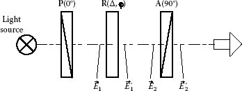
FIGURE 13.3 Linear retarder between crossed linear polarizer and analyzer.

Let us consider a simple system consisting of crossed linear polarizer and analyzer and retarder in between. The setup is shown in Figure 13.3, where P(0°) and A(90°) are linear polarizer and analyzer with transmission axes at 0° and 90° correspondingly, and R(Δ, φ) is a retarder with retardance Δ and slow axis orientation φ. The polarization states at the front and rear faces of the retarder and the analyzer are marked as ${\vec{E}}_{1}, {\vec{E}}_{1}^{'}, {\vec{E}}_{2}$ ${\vec{E}}_{1}, {\vec{E}}_{1}^{'}, {\vec{E}}_{2}$ , and ${\vec{E}}_{2}^{'}$ ${\vec{E}}_{2}^{'}$ .

Polarization of the beam after the polarizer is linear and horizontal. In eigen coordinate system of the retarder with X′-axis parallel to the slow axis, the polarization is also linear but oriented at the angle −φ. Thus, the polarization of the incident beam ${\vec{E}}_{1}$ ${\vec{E}}_{1}$ in the retarder eigen coordinates has the ellipticity angle ε₁ = 0 and the orientation angle ψ = −φ. Using formulas (13.21), we can compute the ratio angle σ₁ = −φ. The phase difference δ₁ = 0 because the polarization is linear.

The retarder introduces an additional phase difference Δ. Therefore, the output beam ${\vec{E}}_{1}^{'}$ ${\vec{E}}_{1}^{'}$ in the retarder eigen coordinates will be described by the ratio angle $σ_{1}^{'} = - φ$ $σ_{1}^{'} = - φ$ and the phase difference $δ_{1}^{'} = Δ$ $δ_{1}^{'} = Δ$ . The corresponding ellipticity and orientation angles of the output polarization ellipse can be obtained by employing Equation 13.20:

${\begin{array}{l} \tan 2 ψ_{1}^{'} = - \tan 2 φ \cos Δ \\ \sin 2 ε_{1}^{'} = \sin 2 φ \sin Δ \end{array} .$ ${\begin{array}{l} \tan 2 ψ_{1}^{'} = - \tan 2 φ \cos Δ \\ \sin 2 ε_{1}^{'} = \sin 2 φ \sin Δ \end{array} .$

(13.23)

In order to find how much light will be transmitted by the analyzer, we have to rotate the polarization ellipse back to the initial coordinate system by adding angle φ to the orientation angle $ψ_{1}^{'}$ $ψ_{1}^{'}$ . The polarization state ${\vec{E}}_{2}$ ${\vec{E}}_{2}$ at the front of the analyzer will be described by the orientation angle $ψ_{2} = ψ_{1}^{'} + φ$ $ψ_{2} = ψ_{1}^{'} + φ$ and ellipticity $ε_{2} = ε_{1}^{'}$ $ε_{2} = ε_{1}^{'}$ . Using expression (13.23), we obtain

${\begin{array}{l} \tan 2 ψ_{2} = \tan 2 (ψ_{1}^{'} + φ) = \frac{\tan 2 ψ_{1}^{'} + \tan 2 φ}{1 - \tan 2 ψ_{1}^{'} \tan 2 φ} = \frac{(1 - \cos Δ) \tan 2 φ}{1 + \tan^{2} 2 φ \cos Δ} . \\ \sin 2 ε_{2} = \sin 2 φ \sin Δ \end{array}$ ${\begin{array}{l} \tan 2 ψ_{2} = \tan 2 (ψ_{1}^{'} + φ) = \frac{\tan 2 ψ_{1}^{'} + \tan 2 φ}{1 - \tan 2 ψ_{1}^{'} \tan 2 φ} = \frac{(1 - \cos Δ) \tan 2 φ}{1 + \tan^{2} 2 φ \cos Δ} . \\ \sin 2 ε_{2} = \sin 2 φ \sin Δ \end{array}$

(13.24)

Intensity of the beam I passed through the linear analyzer with transmission axis at 90° can be found from the ratio

$I = \frac{E_{0 y}^{2}}{E_{0 x}^{2} + E_{0 y}^{2}} I_{0} = \frac{\tan^{2} σ}{1 + \tan^{2} σ} I_{0} = \frac{1}{2} I_{0} (1 - \cos 2 σ),$ $I = \frac{E_{0 y}^{2}}{E_{0 x}^{2} + E_{0 y}^{2}} I_{0} = \frac{\tan^{2} σ}{1 + \tan^{2} σ} I_{0} = \frac{1}{2} I_{0} (1 - \cos 2 σ),$

(13.25)

where I₀ is the intensity of the beam after the polarizer

The ratio angle of the polarization ellipse at the front of the polarizer σ₂ is computed from the first equation of formula (13.21):

$\cos 2 σ_{2} = \cos 2 ε_{2} \cos 2 ψ_{2} .$ $\cos 2 σ_{2} = \cos 2 ε_{2} \cos 2 ψ_{2} .$

In the considered case, after some straightforward trigonometric transformations, we obtain a simple analytical expression for the ratio angle:

$\begin{array}{l} \cos^{2} 2 σ_{2} & = \cos^{2} 2 ε_{2} \cos^{2} 2 ψ_{2} = \frac{1 - \sin^{2} 2 ε_{2}}{1 + \tan^{2} 2 ψ_{2}} = \frac{(1 - \sin^{2} 2 φ \sin^{2} Δ) {(1 + \tan^{2} 2 φ \cos Δ)}^{2}}{{((1 - \cos Δ) \tan 2 φ)}^{2} + {(1 + \tan^{2} 2 φ \cos Δ)}^{2}} \\ = \frac{(1 - \sin^{2} 2 φ \sin^{2} Δ) {(1 + \tan^{2} 2 φ \cos Δ)}^{2}}{(1 + \tan^{2} 2 φ) (1 + \tan^{2} 2 φ \cos^{2} Δ)} = {(\cos^{2} 2 φ + \sin^{2} 2 φ \cos Δ)}^{2} . \end{array}$ $\begin{array}{l} \cos^{2} 2 σ_{2} & = \cos^{2} 2 ε_{2} \cos^{2} 2 ψ_{2} = \frac{1 - \sin^{2} 2 ε_{2}}{1 + \tan^{2} 2 ψ_{2}} = \frac{(1 - \sin^{2} 2 φ \sin^{2} Δ) {(1 + \tan^{2} 2 φ \cos Δ)}^{2}}{{((1 - \cos Δ) \tan 2 φ)}^{2} + {(1 + \tan^{2} 2 φ \cos Δ)}^{2}} \\ = \frac{(1 - \sin^{2} 2 φ \sin^{2} Δ) {(1 + \tan^{2} 2 φ \cos Δ)}^{2}}{(1 + \tan^{2} 2 φ) (1 + \tan^{2} 2 φ \cos^{2} Δ)} = {(\cos^{2} 2 φ + \sin^{2} 2 φ \cos Δ)}^{2} . \end{array}$

(13.26)

Finally, the intensity of the transmitted beam I is reduced to the following formula:

$I = I_{0} \sin^{2} 2 φ \sin^{2} \frac{Δ}{2} .$ $I = I_{0} \sin^{2} 2 φ \sin^{2} \frac{Δ}{2} .$

(13.27)

Formula (13.27) can also be derived using Jones or Muller matrix computation [8]. Advantage of the computation with the polarization ellipse is that the technique does not require employing matrix algebra and complex numbers, and it explicitly shows a transformation of the polarization by each optical element. Of course, not every optical system can be described by a simple analytical expression like formula (13.27). In this case, the ellipse transformation formulas allow to create a numerical mathematical model.

13.6 BASIC OPTICAL SCHEMATICS FOR GENERATING POLARIZED BEAM

13.6.1 COMPLETE POLARIZATION STATE GENERATOR ASSEMBLED WITH INDEPENDENTLY ROTATING LINEAR POLARIZER AND QUARTER-WAVE PLATE

A polarization generator consists of a light source and polarization optical elements to produce a beam of known polarization state. An example of the polarization generator, which is also called the Sénarmont compensator [9], is shown in Figure 13.4. It includes a rotatable linear polarizer P with transmission axis at angle θ and rotatable quarter-wave plate QWP with the slow axis oriented at angle φ. Let us choose the reference axis X perpendicular to the direction of beam propagation. The polarization states at the front and rear faces of the quarter-wave plate are marked as $\vec{E}$ $\vec{E}$ and ${\vec{E}}^{'}$ ${\vec{E}}^{'}$ .

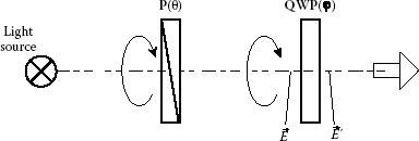
FIGURE 13.4 Complete polarization state generator with independently rotating linear polarizer and quarter-wave plate.

To obtain parameters of the output polarization ellipse ${\vec{E}}^{'}$ ${\vec{E}}^{'}$ we substitute angle difference φ-θ for angle φ, and π/2 for Δ in Equation 13.23, and then add angle φ to the computed ellipse orientation:

${\begin{matrix} ψ^{'} = φ \\ ε^{'} = φ - θ \end{matrix} .$ ${\begin{matrix} ψ^{'} = φ \\ ε^{'} = φ - θ \end{matrix} .$

(13.28)

As it follows from this result, the principal axis of the ellipse is oriented along the slow axis of the quarter-wave plate, and the ellipticity angle is a difference between azimuths of the quarter-wave plate and polarizer. Thus, we can obtain any desired orientation of the polarization ellipse by rotating the quarter-wave plate and any desired ellipticity by turning the polarizer relatively to the quarter-wave plate. For example, the difference φ-θ has to be π/4 for the right circular polarization (ε′ = π/4). Since the generator allows to produce a beam with any polarization state, it is called the complete polarization state generator [10].

Let us consider an interesting case when the quarter-wave plate is oriented at angle φ = π/4. Then, the output polarization ellipse is also oriented at angle ψ′ = π/4. Using inverse Equation 13.21, we can show that the ratio angle σ′ = π/4, which means two orthogonal components $E_{0 x}^{'}$ $E_{0 x}^{'}$ and $E_{0 y}^{'}$ $E_{0 y}^{'}$ have equal amplitudes (see Equation 19). According to Equations 13.21, the phase difference between two components δ’ is determined by difference in the orientation of the polarizer and the quarter-wave plate:

$δ^{'} = 2 ε^{'} = \frac{π}{2} - 2 θ .$ $δ^{'} = 2 ε^{'} = \frac{π}{2} - 2 θ .$

(13.29)

Thus, we can change the phase difference linearly by rotating the polarizer. For example, if θ = π/4, the output components are in-phase. If θ = 0, then the components are shifted by π/2 (quarter-wave). If the polarizer is oriented at −π/4, then the output electric vectors are antiphase (half-wave shift). Polarizer at −π/2 produces phase shift 3π/2 (three quarter-wave). This feature of the Sénarmont compensator is often employed in phase shifting interferometry and birefringence mapping techniques.

13.6.2 COMPLETE POLARIZATION STATE GENERATOR ASSEMBLED WITH JOINTLY ROTATING LINEAR POLARIZER AND VARIABLE RETARDER

Another optical configuration of polarization state generator is presented in Figure 13.5. Linear polarizer P and variable retarder VR are mounted in the rotatable body. The angle between the transmission axis of the polarizer and the slow axis of the retarder is π/4. As a variable retarder, one can use Babinet–Soleil compensator [2,3,9], Berek compensator [3,9,11] or its analog made of quartz [12], the Ehringhaus compensator [9,13], liquid crystal cell [7,14], electro-optical or piezo-optical modulator [2,5], for instance. A phase difference Δ of the retarder can be adjusted. The variable retarder is turned together with the polarizer. Orientation of the polarizer transmission axis is θ. The retarder slow axis orientation is θ + π/4 accordingly. The polarization states at the front and rear faces of the variable retarder are shown as $\hat{E}$ $\hat{E}$ and ${\vec{E}}^{'}$ ${\vec{E}}^{'}$ .

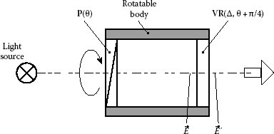
FIGURE 13.5 Complete polarization state generator with jointly rotating linear polarizer and variable retarder.

For the analysis of the generator, we use the coordinate system in which X′-axis is parallel to the transmission axis of the polarizer. Parameters of the output polarization ellipse ${\vec{E}}^{'}$ ${\vec{E}}^{'}$ are determined from formula (13.24) at ϕ = π/4 and then angle θ is added to the computed ellipse orientation:

${\begin{matrix} ψ^{'} = θ \\ ε^{'} = Δ / 2 \end{matrix} .$ ${\begin{matrix} ψ^{'} = θ \\ ε^{'} = Δ / 2 \end{matrix} .$

(13.30)

As one can see, the ellipticity angle of the output beam equals a half of retardance, and the principal axis of the ellipse is oriented along the transmission axis of the polarizer. For example, if the retardance is quarter-wave (Δ = π/2), then the output beam is RCP. Rotating the entire setup can produce any desired orientation of the polarization ellipse, and any ellipticity can be obtained by changing the retardance of the variable retarder. Using a fast variable retarder, such as a liquid crystal cell or electro-optic crystal, allows quick control of the ellipticity of the output beam.

13.6.3 COMPLETE POLARIZATION STATE GENERATOR ASSEMBLED WITH ROTATING LINEAR POLARIZER AND FIXED VARIABLE RETARDER

In order to control the introduced retardance, a variable retarder requires either mechanical movement of its components or application of electrical voltage. Therefore, the retarder’s rotating mechanism could be bulky and complicated to build. Sometimes, it is necessary to quickly change the polarization ellipse orientation, not its ellipticity. Recently, we proposed a new complete polarization state generator with one variable retarder, which is fixed [15]. New generator allows rapid change in the polarization ellipse orientation.

A schematic of the proposed polarization state generator is shown in Figure 13.6. It contains in-series rotatable polarizer P and fixed variable retarder VR, which introduces a phase shift Δ and quarter-wave plate QWP. Let us choose the slow axis of the quarter-wave plate as X-axis of the Cartesian coordinates. The transmission axis of the polarizer is inclined at an azimuth θ from the X-axis. For simplicity of the description, we consider angle range −π/4 ≤ θ ≤ π/4. The polarization states at the front and rear faces of the variable retarder and quarter-wave plate are noted as ${\vec{E}}_{1}, {\vec{E}}_{1}^{'}, {\vec{E}}_{2}$ ${\vec{E}}_{1}, {\vec{E}}_{1}^{'}, {\vec{E}}_{2}$ , and ${\vec{E}}_{2}^{'}$ ${\vec{E}}_{2}^{'}$ , respectively.

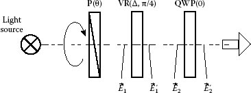
FIGURE 13.6 Complete polarization state generator with rotating linear polarizer and fixed variable retarder.

Electric vector ${\vec{E}}_{1}$ ${\vec{E}}_{1}$ represents a linear vibration at angle θ − π/4 to the slow axis of the variable retarder, and it is described by the polarization ellipse with the following parameters in the eigen coordinates of the retarder:

${\begin{matrix} ψ_{1} = θ - π / 4 \\ ε_{1} = 0 \end{matrix} .$ ${\begin{matrix} ψ_{1} = θ - π / 4 \\ ε_{1} = 0 \end{matrix} .$

(13.31)

The corresponding polarization components σ₁ and δ₁ are obtained with formula (13.21):

${\begin{matrix} σ_{1} = θ - π / 4 \\ δ_{1} = 0 \end{matrix} .$ ${\begin{matrix} σ_{1} = θ - π / 4 \\ δ_{1} = 0 \end{matrix} .$

(13.32)

The variable retarder creates phase delay Δ between the slow and fast components. Then, the output electric vector ${\vec{E}}_{1}^{'}$ ${\vec{E}}_{1}^{'}$ has the next ratio angle and retardation:

${\begin{matrix} σ_{1}^{'} = θ - π / 4 \\ δ_{1}^{'} = Δ \end{matrix} .$ ${\begin{matrix} σ_{1}^{'} = θ - π / 4 \\ δ_{1}^{'} = Δ \end{matrix} .$

(13.33)

Shape and orientation of the interim polarization ellipse ${\vec{E}}_{2}$ ${\vec{E}}_{2}$ in eigen coordinate of the quarter-wave plate can be obtained by replacing δ with Δ and σ with θ − π/4 in Equation 13.20 and then adding π/4 to the orientation angle:

${\begin{matrix} \tan 2 ψ_{2} = \tan 2 θ / \cos Δ \\ \sin 2 ε_{2} = - \cos 2 θ \sin Δ \end{matrix} .$ ${\begin{matrix} \tan 2 ψ_{2} = \tan 2 θ / \cos Δ \\ \sin 2 ε_{2} = - \cos 2 θ \sin Δ \end{matrix} .$

(13.34)

The corresponding ratio σ₂ and phase shift δ₂ at the entrance of the quarter-wave plate can be found with formula (13.21). Then, the quarter-wave plate adds retardation π/2 to the phase shift δ (δ′ = δ + π/2) and keeps the ratio constant (σ′ = σ):

${\begin{matrix} \cos 2 σ_{2}^{'} = \cos 2 ε_{2} \cos 2 ψ_{2} \\ \tan δ_{2}^{'} = - \sin 2 ψ_{2} / \tan 2 ε_{2} \end{matrix} .$ ${\begin{matrix} \cos 2 σ_{2}^{'} = \cos 2 ε_{2} \cos 2 ψ_{2} \\ \tan δ_{2}^{'} = - \sin 2 ψ_{2} / \tan 2 ε_{2} \end{matrix} .$

(13.35)

The output polarization ellipse ${\vec{E}}_{2}^{'}$ ${\vec{E}}_{2}^{'}$ can be computed in the following way (see Equation 13.20):

${\begin{matrix} \tan 2 ψ_{2}^{'} = \tan 2 σ_{2}^{'} \cos δ_{2}^{'} \\ \sin 2 ε_{2}^{'} = \sin 2 σ_{2}^{'} \sin δ_{2}^{'} \end{matrix} .$ ${\begin{matrix} \tan 2 ψ_{2}^{'} = \tan 2 σ_{2}^{'} \cos δ_{2}^{'} \\ \sin 2 ε_{2}^{'} = \sin 2 σ_{2}^{'} \sin δ_{2}^{'} \end{matrix} .$

(13.36)

After squaring Equations 13.34 through 13.36 and sequential substitution of the variables, we receive simple straightforward formulas that connect ellipticity and orientation of the output polarization, $ε_{2}^{'}$ $ε_{2}^{'}$ and $ψ_{2}^{'}$ $ψ_{2}^{'}$ , with the polarizer’s orientation and variable retarder’s phase shift, θ and Δ:

${\begin{matrix} ψ_{2}^{'} = Δ / 2 \\ ε_{2}^{'} = θ \end{matrix} .$ ${\begin{matrix} ψ_{2}^{'} = Δ / 2 \\ ε_{2}^{'} = θ \end{matrix} .$

(13.37)

Thus, the proposed polarization generator can produce any polarization state of the output beam:

${\begin{matrix} 0 \leq ψ_{2}^{'} \leq π, if 0 \leq Δ \leq 2 π \\ - π / 4 \leq ε_{2}^{'} \leq π / 4, if - π / 4 \leq θ_{2} \leq π / 4 \end{matrix} .$ ${\begin{matrix} 0 \leq ψ_{2}^{'} \leq π, if 0 \leq Δ \leq 2 π \\ - π / 4 \leq ε_{2}^{'} \leq π / 4, if - π / 4 \leq θ_{2} \leq π / 4 \end{matrix} .$

The desired ellipticity angle $ε_{2}^{'}$ $ε_{2}^{'}$ can be achieved by rotating the polarizer, and the major axis orientation $ψ_{2}^{'}$ $ψ_{2}^{'}$ is determined by phase shift of the variable retarder. So, using a fast variable retarder, such as a liquid crystal cell or electro-optic crystal, allows quick control of the orientation of the output polarization ellipse.

We have also derived formula (13.37) by multiplication of Jones matrices followed by a complex vector conjugation [15]. The mentioned publication describes techniques for fast and sensitive differential measurements of 2D birefringence distribution, which utilize the complete polarization state generator with single variable retarders.

13.6.4 COMPLETE POLARIZATION STATE GENERATOR ASSEMBLED WITH FIXED LINEAR POLARIZER AND TWO VARIABLE RETARDERS (TYPE 1)

The earlier described polarization generators have two or one rotatable component. Arrangement of the complete polarization state generator without any mechanical rotation was proposed by Yamaguchi and Hasunuma [2,16]. A schematic of the Yamaguchin–Hasunuma compensator, which consists of two variable retarders, is shown in Figure 13.7. Two liquid crystal cells LCA and LCB are used as variable wave plate whose retardations α and β are controlled by voltages. The slow axes of LCA and LCB are chosen at π/4 and 0 (parallel) orientations from the transmission axis of the polarizer P. The polarization states at the front and rear faces of the liquid crystal cells are noted as ${\vec{E}}_{1}, {\vec{E}}_{1}^{'}, {\vec{E}}_{2}$ ${\vec{E}}_{1}, {\vec{E}}_{1}^{'}, {\vec{E}}_{2}$ , and ${\vec{E}}_{2}^{'}$ ${\vec{E}}_{2}^{'}$ . Instead of liquid crystal cells, one can use other kinds of variable retarders as mentioned earlier.

Shape and orientation of the polarization ellipse ${\vec{E}}_{2}$ ${\vec{E}}_{2}$ can be obtained by substitution φ = π/4 and replacing Δ with α in Equation 13.24:

${\begin{matrix} ψ_{2} = 0 \\ ε_{2} = α / 2 \end{matrix} .$ ${\begin{matrix} ψ_{2} = 0 \\ ε_{2} = α / 2 \end{matrix} .$

(13.38)

The corresponding polarization components σ₂ and δ₂ are obtained with formula (13.21):

${\begin{matrix} σ_{2} = α / 2 \\ δ_{2} = π / 2 \end{matrix} .$ ${\begin{matrix} σ_{2} = α / 2 \\ δ_{2} = π / 2 \end{matrix} .$

(13.39)

The second variable retarder introduces phase difference β. Then, the output beam ${\vec{E}}_{2}^{'}$ ${\vec{E}}_{2}^{'}$ will have the following ratio angle and phase difference:

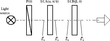
${\begin{matrix} σ_{2}^{'} = α / 2 \\ δ_{2}^{'} = β + π / 2 \end{matrix} .$ ${\begin{matrix} σ_{2}^{'} = α / 2 \\ δ_{2}^{'} = β + π / 2 \end{matrix} .$

(13.40)

FIGURE 13.7 Complete polarization state generator with fixed linear polarizer and two variable retarders (type 1).

The relative amplitude of the X- and Y-polarization components of the output light is controlled by α, whereas the phase difference of the same components is controlled by β. Therefore, by controlling the voltages applied to LCA and LCB, any state of polarization for the output beam can be generated.

The corresponding ellipticity and orientation angles of the polarization ellipse can be computed from Equation 13.20:

${\begin{matrix} ψ_{2}^{'} = - \frac{1}{2} arctan (\tan α \sin β) \\ ε_{2}^{'} = \frac{1}{2} arcsin (\sin α \cos β) \end{matrix}$ ${\begin{matrix} ψ_{2}^{'} = - \frac{1}{2} arctan (\tan α \sin β) \\ ε_{2}^{'} = \frac{1}{2} arcsin (\sin α \cos β) \end{matrix}$

(13.41)

The inverse transformation, which shows what phase shifts α and β should be applied in order to obtain the required ellipticity and orientation angles of the output beam $ε_{2}^{'}$ $ε_{2}^{'}$ and $ψ_{2}^{'}$ $ψ_{2}^{'}$ , is the following:

${\begin{matrix} α = arccos (\cos 2 ψ_{2}^{'} \cos 2 ε_{2}^{'}) \\ β = - \arctan (\sin ψ_{2}^{'} / \tan 2 ε_{2}^{'}) \end{matrix} .$ ${\begin{matrix} α = arccos (\cos 2 ψ_{2}^{'} \cos 2 ε_{2}^{'}) \\ β = - \arctan (\sin ψ_{2}^{'} / \tan 2 ε_{2}^{'}) \end{matrix} .$

(13.42)

We have also derived formula (13.41) by multiplication of Jones matrices followed by a complex vector conjugation [17]. This publication describes techniques for fast and sensitive differential measurements of 2D birefringence distribution, which utilize the complete polarization state generator with two variable retarders. The corresponding systems for quantitative birefringence imaging are currently manufactured by Perkin Elmer (http://www.perkinelmer.com). The polarization generator is mentioned as a precision liquid crystal compensator in the company’s website.

13.6.5 COMPLETE POLARIZATION STATE GENERATOR ASSEMBLED WITH FIXED LINEAR POLARIZER AND TWO VARIABLE RETARDERS (TYPE 2)

Disadvantage of the Yamaguchi–Hasunuma setup is that parameters of the output polarization ellipse are connected with retarder’s phase shifts by quite complicated trigonometric Equation 13.41. Also, in order to change the ellipse orientation angle or ellipticity only, we have to change phase shifts of both the retarders (see Equation 13.42).

In order to simplify control of the output polarization ellipse and provide more functionality, we are proposing another type of the complete polarization state generator assembled with fixed linear polarizer and two variable retarders, which is shown in Figure 13.8. It contains, in series, a fixed polarizer P, two variable retarders VR1 and VR2, and polymer quarter-wave retardation film QWF. The two variable retarders introduce retardations α and β, respectively. The slow axes of VR1 and VR2 are chosen at π/4 and 0 (parallel) orientations from the transmission axis of the polarizer P. The slow axis of quarter-wave film QWF has direction π/4. Of course, instead of the quarter-wave film, we could employ a quarter-wave plate, as in the polarization state generators described earlier. Using a quarter-wave retardation film allows to simplify the generator.

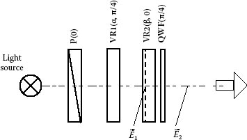
FIGURE 13.8 Complete polarization state generator with fixed linear polarizer and two variable retarders (type 2).

The proposed setup could be considered as a sequential combination of two polarization state generators with single variable retarder each (see Section 13.6.3), where retardation of the second retarder consists of two parts, π/2 and β-π/2. The slow axes of both the parts are oriented at 0 rad. The polarizer P, first variable retarder VR1, and the first quarter-wave part of the second variable retarder VR2 form the first polarization state generator, which produces linearly polarized beam ${\vec{E}}_{1}$ ${\vec{E}}_{1}$ with orientation angle ψ₁ = α/2 (see Equation 13.37). The second part of retarder VR2 with retardation β-π/2 and quarter-wave film QWF creates the second polarization state generator. Polarization plane of beam ${\vec{E}}_{1}$ ${\vec{E}}_{1}$ is turned by angle θ = ψ₁ − π/4 = α/2 − π/4 relatively to the slow axis of the quarter-wave film. Then, according to Equation 13.37, the output beam ${\vec{E}}_{2}$ ${\vec{E}}_{2}$ has the following ellipticity and orientation angles of the polarization ellipse, ε₂ and ψ₂:

${\begin{matrix} ψ_{2} = β / 2 \\ ε_{2} = α / 2 - π / 4 \end{matrix} .$ ${\begin{matrix} ψ_{2} = β / 2 \\ ε_{2} = α / 2 - π / 4 \end{matrix} .$

(13.43)

The inverse transformation, which shows what phase shifts α and β should be applied in order to obtain the required ellipticity and orientation angles of the output beam ε₂ and ψ₂, is the following:

${\begin{matrix} α = 2 ε_{2} + π / 4 \\ β = 2 ψ_{2} \end{matrix} .$ ${\begin{matrix} α = 2 ε_{2} + π / 4 \\ β = 2 ψ_{2} \end{matrix} .$

(13.44)

The ellipticity and orientation angles of the output beam are directly determined by retardations of the first and second variable retarders, α and β, respectively.

13.7 CONCLUSION

In this chapter, we gave the classical description of the polarization of monochromatic light. The direct and inverse equations for transformations of the polarization ellipse were derived. An example of the application of the obtained formulas for the analysis of beam propagation through crossed polarizers and a wave plate was given. Basic optical schematics for generating and analyzing any polarization states were presented.

ACKNOWLEDGMENT

This publication was made possible by Grant Number R01-GM101701 from the National Institute of General Medical Sciences, the National Institutes of Health. Its contents are solely the responsibility of the author and do not necessarily represent the official views of the National Institute of General Medical Sciences or the National Institutes of Health.

REFERENCES

1. Shurcliff, W.A., Polarized Light: Production and Use, Harvard University Press, Cambridge, MA, 1962.

2. Azzam, R.M.A. and Bashara, N.M., Ellipsometry and Polarized Light, Elsevier Science, Amsterdam, the Netherlands, 1987.

3. Born, M. and Wolf, E., Principles of Optics, 7th edn., Cambridge University Press, New York, 1999.

4. Ramachandran, G.N. and Ramaseshan, S., Crystal optics, in Handbuch der Physik, vol. 25/1, S. Flugge, ed., Springer, Berlin, Germany, 1961.

5. Yariv, A. and Yeh, P., Optical Waves in Crystals: Propagation and Control of Laser Radiation, John Wiley & Sons, New York, 1984.

6. Yeh, P., Optical Waves in Layered Media, John Wiley & Sons, New York, 1988.

7. Robinson, M., Chen, J., and Sharp, G.D., Polarization Engineering for LCD Projection, John Wiley & Sons, New York, 2005.

8. Gerrard, A. and Burch, J.M., Introduction to Matrix Methods in Optics, John Wiley & Sons, New York, 1975.

9. Hartshorne, N.H. and Stuart A., Crystals and the Polarizing Microscope, 4th edn., Edward Arnold, London, U.K., 1970.

10. Hauge, P.S., Recent development in instrumentation in ellipsometry, Surf. Sci., 96, 108–140, 1980.

11. Rinne, F. and Berek, M., Anleitung zu Optischen Untersuclhungen mit dem Polarizationsmikroskop, Schweizerbart’sche Verlagsbuchhandlung, Stuttgart, Germany, 1953.

12. Shribak, M., Use of gyrotropic birefringent plate as quarter-wave plate, Sov. J. Opt. Technol., 53, 443–446, 1986.

13. Holmes, D.A., Wave optics theory of rotary compensators, J. Opt. Soc. Am., 54, 1340–1347, 1964.

14. Scharf, T., Polarized Light in Liquid Crystals and Polymers, John Wiley & Sons, Hoboken, NJ, 2007.

15. Shribak, M., Complete polarization state generator with one variable retarder and its application for fast and sensitive measuring of two-dimensional birefringence distribution, J. Opt. Soc. Am. A, 28, 410–419, 2011.

16. Yamaguchi, T. and Hasunuma, H., A quick response recording ellipsometer, Sci. Light, 16(1), 64–71, 1967.

17. Shribak, M. and Oldenbourg, R., Techniques for fast and sensitive measurements of two-dimensional birefringence distributions, Appl. Opt., 42, 3009–3017, 2003.

..................Content has been hidden....................

You can't read the all page of ebook, please click here login for view all page.

Table of Contents for Chapter 13 Polarization

Create new playlist

Sign In

Sign Up

Table of Contents for
Chapter 13 Polarization