
CONTENTS
24.2 Laser Doppler Velocimetry
24.2.2 Optical Arrangement and SNR
24.3 Particle Image Velocimetry
24.3.1 Principle of PIV Measurement
24.3.2 Classification of PIV Techniques
24.3.4 Typical Application: Measurement of a Turbulent Boundary Layer.
24.4.2 Typical Application: Flow behind an Axial-Fan
24.5.1 Film-Based Holographic PIV
24.5.2 Digital Holographic PTV
Fluid is the common name given to gas and liquid. Flow cannot be at rest when there is shearing stress. In addition, most flows occurring in nature and engineering applications are turbulent, in which flow velocity varies rapidly with randomness and irregularity in space and time, difficult to predict accurately. To understand the turbulent flow motion in detail, we need to measure the quantitative velocity profile or distribution of the flow.
There are various kinds of flow-velocity measurement techniques. The simplest means is to use a measuring probe such as a pitot tube or a hot-wire probe. The velocity probe is positioned at one point or at multiple points in a flow field to be measured. It usually disturbs the flow and changes the flow downstream. In addition, it requires elaborated effort to obtain velocity components separately and to measure flow reversal. This point-wise measurement technique is difficult to apply to unsteady or transient flows [1].
On the other hand, optical methods do not disturb the flow and measure velocity components precisely. Light or sound waves undergo a Doppler shift when they are scattered off from particles in a moving fluid. The Doppler frequency shift is proportional to the speed of the scattering particles. By measuring the frequency difference between the scattered and unscattered waves, the flow velocity can be measured. Laser doppler velocimetry (LDV) has been used as a reliable and representative velocity-measuring device. Flow velocity is measured precisely by detecting the variation of Doppler frequency of light scattered by tracer particles seeded in the flow at a small measurement volume formed by laser-beam crossover. LDV does not disturb the flow and no velocity calibration is required. In addition, the velocity components of a flow, even with flow reversal, can be measured separately. However, the expensive LDV system requires precise optical arrangement and seeding of tracer particles [2].
Recently, quantitative optical flow visualization has become an indispensable tool in the investigation of complex flow structures. Recent advances in laser, computer, and digital image-processing techniques have made it possible to extract quantitative flow information from visualized flow images of tracer particles [3]. Particle image velocimetry (PIV) is one of the most important achievements of flow diagnostic technologies in the modern history of fluid mechanics. The PIV technique measures the whole velocity field in a plane by dividing the displacements ΔX and ΔY of tracer particles with the time interval Δt during which the particles have been displaced. Since the flow velocity is inferred from the particle velocity, it is important to select tracing particles that will follow the flow motion within an acceptable uncertainty without affecting the fluid properties that are to be measured.
The PIV velocity-field measurement method is a very powerful tool to measure whole flow of field information for various flows and to understand the flow structure, compared with point-wise velocity measurement techniques such as hot wire or LDV. Furthermore, other physical properties such as vorticity, deformation, and forces can also be derived easily from the PIV data. Recently, PIV and particle tracking velocimetry (PTV) have been used as reliable and powerful two-dimensional velocity-field measurement techniques.
In this chapter, the basic principle and typical applications of LDV and PIV methods are explained. As a three-dimensional (3D) velocity-field measurement technique, the stereoscopic PIV (SPIV) and holographic PIV (HPIV) techniques are briefly introduced in this chapter. In addition, a micro-PIV method and its simple application are also discussed.
24.2 LASER DOPPLER VELOCIMETRY
LDV is an optical method used to measure a local velocity of a moving fluid. The LDV utilizes the Doppler effect by detecting the Doppler frequency shift of laser light that has been scattered by tracer particles moving with the fluid. As one of the major advantages of the LDV system, the flow being measured is not affected by a velocity probe. Since the velocity information is derived based on a simple geometric correlation, calibration process is unnecessary. Furthermore, the direction of the flow velocity being measured is determined directly by the optical arrangement. Another advantage is its high-spatial and temporal-resolution qualities. However, the LDV system has drawbacks such as highly complicated optical setups and bothersome signal processing. The LDV signal obtained from a photodetector contains a considerable noise.
In its basic form, the LDV system consists of a laser, focusing and receiving optics, a photodetector, a signal processor, and data-processing computer as shown in Figure 24.1. At first, a laser provides a collimated and coherent light. A beam splitter divides the laser light into two coherent beams. Two laser beams are crossed at a point where the flow velocity is to be measured. The fluid is seeded with fine particles of typically 0.1 to ~10 μm in diameter. Tracer particles are seeded in the fluid scatter light in all directions while the laser beam goes through the beam crossover. This scattered light can be collected from any direction by a photodetector (or photomultiplier). The frequency of the scattered light collected by a photodetector is Doppler-shifted and the shifted frequency is referred to as the Doppler frequency of the flow. The electrical signal converted by a photodetector goes through a signal processor, then the signal processor converts the Doppler frequency into a voltage signal. At last, data processor converts the output of the signal processor into readable flow information [4].
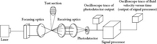
FIGURE 24.1 Basic LDV system configuration.
The basic principle of LDV measurement is the Doppler frequency shift of the scattered light from tracer particles seeded in the flow. As a tracer particle moves with the fluid flow, its relative motion to the laser beam determines the degree of the frequency shift, compared with the frequency of the incident laser light. In practice, however, the real value of the frequency shift is very small, compared to the frequency of the incident laser beam. Therefore, a process known as optical heterodyne is commonly used to determine the amount of frequency shift accurately.
The scattered light from a tracer particle that undergoes the optical heterodyne has a form of beat called Doppler burst as shown in the upper left side of Figure 24.2. The measuring volume has an ellipsoidal shape. From the Doppler burst and the fringe pattern, the velocity of a tracer particle, that is, the local velocity of the flow, is determined by the following equation:
|
The fringe spacing (df) depends on the wavelength of incident laser light (λ) and half angle (κ). The wavelength of lasers is well known accurately (0.01% or better). Therefore, the Doppler frequency (fD) is proportional to the particle velocity.
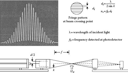
FIGURE 24.2 Doppler burst signal and fringe pattern at the laser beam crossing point.
24.2.2 OPTICAL ARRANGEMENT AND SNR
Depending on the location of receiving optics and photodetector, collecting the scattering light, the LDV system is classified into the forward-scatter mode and the backscatter mode as shown in Figure 24.3. The collection optics with the dual-beam LDV system can be placed at any angle and gives the same frequency. However, the signal quality and intensity of the scattered light is affected greatly by an angle θ between the receiving optics and the incident laser beam. While on-axis backscatter and forward-scatter modes are employed most often, the off-axis arrangement can reduce the effects of flare and reflections and decrease the length of the measuring volume.
As the tracer particles pass through the fringe pattern, they scatter light that appears as a blinking signal. The frequency of this on-and-off signal is proportional to the velocity component perpendicular to the planes of the fringes. As shown in Figure 24.4, the scattering light depends on the location of receiving optics for collecting scattering light with respect to the incident light. The light scattered in the forward direction (θ = 0°) has the largest intensity value, about two orders of magnitude larger than the backscatter mode (θ = 180°). When small tracer particles (about 1 μm) are used, the forward-scatter mode is useful, because the light intensity is much stronger than the backscatter mode. However, the backscatter mode has to be employed in the experimental facilities in which back side has space restrictions to locate the receiving optics or a transparent window. The LDV system of backscatter mode is easy to carry out experiments and its optical alignment is not so difficult. However, since the scattering light intensity is weak, the selection of tracer particles and the signal-processing procedure should be done carefully.
The signal-to-noise ratio (SNR) of the Doppler signal obtained from a photodetector should be increased to acquire accurate information of the flow, since the overall performance of the LDV system is largely affected by the SNR of the LDV signal. The SNR of Doppler signal is related with optical factors such as laser power, optical arrangement, performance of photodetector, and seeding particles as a source of scattering light. Therefore, we need to accurately select proper values of these governing factors accurately. Using the Mie-scattering theory, the SNR of LDV signal can be expressed as follow:
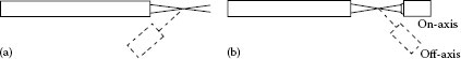
FIGURE 24.3 Optical setups for (a) back scatter mode and (b) forward scatter mode.
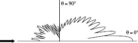
FIGURE 24.4 Intensity of the scattered light according to the angle between an incident light and a photodetector.
where
Da is the collection aperture diameter of receiving lens (mm)
DP is the particle diameter (μm)
Ḡ is the average gain of scattering light
h is the Plank’s constant (6.6 × 10⁻³⁴ J s)
P0 is the power of each laser beam in dual beam LDV (W)
ra is the distance between the measuring volume and receiving lens (mm)
is the Doppler signal visibility
ΔF is the bandwidth of photomultiplier (MHz)
ηq is the quantum efficiency of photomultiplier
υ0 is the frequency of the laser light
In the above equation, the terms [A], [B], and [C] represent the effects of laser source and photomultiplier, the effects of the optical arrangement of the LDV system, and the physical properties of seeding particles, respectively. In [A], the SNR is proportional to the power of laser beam, because commercial photodetectors have a nearly fixed value of efficiency. In [B], SNR is increased with the increase of the diameter of focusing lens and with the decrease of the measuring volume.
Since the LDV measures only the velocity of the tracer particles instead of the flow itself, the properties of the tracer particle should be selected carefully to secure the measurement accuracy. The most important property is the particle size. As the size of the tracer particle increases, the intensity of the scattered light increases, that is, increasing SNR of the Doppler signal. As the size of the tracer particle increases, on the other hand, the fidelity of the tracer particles to follow the flow accurately is diminished. In addition, pedestal noise is increased and frequency response of particles to the flow is decreased.
When a particle whose diameter is larger than the fringe spacing passes, the measuring volume or incomplete heterodyne mixing on the photodetector occurs due to phase difference of scattering light. That is, the smaller particle is required for good traceability to the highly turbulent flow; however, the bigger particle is needed to produce strong light scattering. It is difficult to satisfy the above two conditions together.
The particle concentration will influence the data rate, that is, the ability to follow the time history of the flow. The signal characteristics depend on the average number of particles in the measuring volume. Clean Doppler signal can be obtained, when the number of seeding tracer particles is maintained as small as possible, but, enough to operate the signal processor at least. Dropout phenomenon occurs when the number of particles in the measuring volume is too little. On the other hand, if excessive particles, more than two particles in the measuring volume, are supplied, the mutual interaction between particles influences the measured velocity data. Therefore, the size and number of particles should be properly selected according to the given experimental condition. The ideal number of particles is one particle in the measuring volume. For this ideal particle concentration, the output signal of photodetector shows a normal Gaussian distribution.
In addition, the other requisites of scattering particles include spherical shape, good light scattering surface, cheap and easy to generate, noncohesive, nontoxic, nonerosive, nonadhesive on the measuring window, with monodispersity, and are chemically inactive.
The tracer particle can be generated by atomization, fluidization, chemical reaction, combustion, and sublimation. For air seeding techniques, the condensation of liquid such as water, and atomization of low vapor-pressure materials (e.g., olive oil) by supplying compressed air are most popular.
The signal processor of the LDV system is required to have a high frequency range and high temporal resolution. The signal processor also needs to have an ability to extract effective Doppler signal from LDV signal embedded in noises.
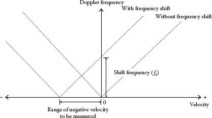
FIGURE 24.5 Frequency shift for measuring negative velocity of flow.
The signal processors are classified into three types, depending on how to extract the Doppler frequency from the LDV signal. The tracker-type processor tracks the instantaneous frequency signal to calculate the Doppler frequency. On the other hand, the counter-type processor measures the frequency of LDV signals by counting accurately the time duration of an integer number of cycles. Lastly, the spectrum analyzer calculates the power spectrum of LDV signal and determines the peak frequency as a Doppler frequency.
LDV system has the ability of measuring negative velocity of flow reversal. This is possible by shifting the frequency of one of the two incident laser beams and translating fringes in the measuring volume as shown in Figure 24.5. Frequency shifting is a very useful tool in LDV measurements for improving the dynamic range and allowing the measurement of flow reversal. In principle, it can be utilized with any scattering mode. In the dual-beam LDV system, a tracer particle in the measuring volume gives the frequency shift (fs). If the velocity increases in the direction of fringe movement, the Doppler frequency will decrease. If it is opposite to the fringe movement, the frequency will increase.
In practical applications of LDV systems, a fiber-optic LDV system as shown in Figure 24.6 has several advantages. For conventional LDV systems, the laser source is so heavy and bulky that it is difficult to traverse the whole LDV system to the measurement point. The use of optical fibers connecting the laser source with the optical head of the LDV system makes it easy to locate the optical head to harsh environments such as hot or corrosive fluids. In addition, the LDV probe head is submersible and the electronic components of the LDV system can be separated from the measuring fluid-flows for electrical-noise immunity [5].
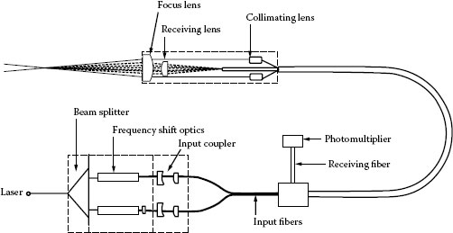
FIGURE 24.6 Configuration of a fiber-optic LDV system. (Courtesy of TSI Incorporated, Shoreview, MN.)
24.3 PARTICLE IMAGE VELOCIMETRY
Most flow phenomena encountered in nature or industrial applications are unsteady and 3D turbulent flows. In order to analyze such turbulent flow phenomena, whole velocity-field information is required as a function of time. However, none of the currently available point-wise experimental techniques can provide such flow information. Recent advances in numerical simulations make us understand the sophisticated aspects of flow dynamics [6]. However, it is usually limited to simple geometries and relatively low Reynolds numbers yet. The recent advances in the digital image-processing method, computer science, and optics have opened a new paradigm for measuring whole velocity field of a flow by using a digital flow-assessment technique, such as PIV [3,7]. Nowadays, 2D PIV and PTV methods are widely used as a reliable velocity-field measurement technique. In addition, by statistical analysis of instantaneous 2D velocity fields, it is possible to extract the spatial distributions of turbulent quantities of turbulent flows having complicated flow structures.
24.3.1 PRINCIPLE OF PIV MEASUREMENT
Figure 24.7 shows the basic principle of a PIV velocity-field measurement technique that extracts whole velocity-field information by processing the flow images of tracer particles seeded in the flow. The PIV system consists of a laser, optics, tracer particles, and an image-recording device. To measure the whole velocity field in a measurement plane accurately, at first, tiny tracer particles that have good traceability should be seeded in the flow. Thereafter, the test section is illuminated by a thin laser light sheet and the illuminated light is scattered by tracer particles in the flow. The laser light sheet is formed by passing the laser beam through optical components such as cylindrical or spherical lens.
A particle image illuminated by the thin laser light sheet is captured by an image-recording device such as a digital charge-coupled device (CCD) camera at a time t = t0. Second particle image is obtained at time t = t0 + Δt after a small time interval Δt. The time interval should be adjusted according to the velocity of the measuring flow. From the two consecutive flow images stored in the computer memory as 2D image data, the displacement vector (ΔS) of each tracer particle can be extracted by using a digital image-processing technique. Here, the displacements of individual particles are presented as a function of space and time, ΔS(x, y; t). The velocity vector U(x, y) can be obtained by dividing the displacement vector ΔS with the time interval Δt [8].
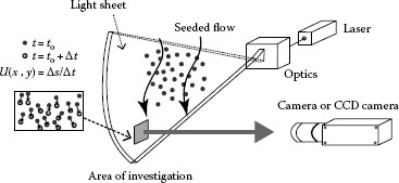
FIGURE 24.7 Basic principle of PIV velocity-field measurement technique.
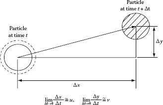
FIGURE 24.8 Calculation of velocity vector of a moving particle.
Figure 24.8 shows how to obtain the velocity vector of tracer particles moved during the time interval Δt of the PIV velocity-field measurement. The stream-wise (x) velocity component u and vertical (y) velocity component v are obtained by dividing the displacement components (Δx, Δy) of the particle, which moved with the flow during the time interval Δt, with the time interval Δt as follows:
Here, the displacement Δx should be small enough so that Δx/Δt is a good approximation of the stream-wise velocity component u. This means that the trajectory of the tracer particle should be almost a straight line during the time interval Δt, and the velocity of the tracer particle should be nearly constant along the trajectory. It has been known that these conditions can be satisfied if the time interval Δt is small, compared to the Taylor microscale in the Lagrangian velocity field. However, if the time interval Δt is too small, the particle displacement ΔS also becomes small and the measurement uncertainty of ΔS increases [9].
The velocity field of a flow can be measured by three steps: capturing the particle images, extraction of velocity vectors, and representation of the extracted velocity field. For the particle imagecapturing procedure, the proper tracer particles must be selected and the measurement plane is illuminated with a thin laser light sheet. Thereafter, the images of scattered particles are captured by a CCD or complementary metal-oxide semiconductor (CMOS) camera that is installed perpendicular to the laser light sheet. The size and concentration of tracer particles, the exposure time of camera, and the time interval Δt of two consecutive flow images should be set accurately according to the experimental condition and flow information to be measured.
There are several PIV/PTV techniques for measuring velocity vectors from the captured particle images according to the method of determining particle displacements. In order to apply a PIV technique to measure accurately the velocity fields of turbulent flows that change suddenly in space and time, an exact PIV/PTV algorithm should be developed to extract velocity vectors accurately and the effort to reduce the total calculation time is likewise necessary. In addition, error vectors contained in the velocity field measured should be removed in the procedure of extracting velocity vectors.
The post-processing procedure consists of the calculation of vorticity or rate of strain field from the instantaneous velocity field and ensemble averaging of many instantaneous velocity filed samples to obtain various flow parameters such as the turbulence intensity, Reynolds shear stress, and turbulent kinetic energy. In addition, the dissipation rate or spatial distribution of pressure can also be calculated by utilizing the governing equations of the fluid flows.
24.3.2 CLASSIFICATION OF PIV TECHNIQUES
The PIV techniques are classified into particle streak velocimetry (PSV), PIV, PTV, and LSV (laser speckle velocimetry), depending on how to obtain the displacement vector of tracer particles during the time interval Δt.
The PSV method extracts the velocity vectors by dividing the streak lines of tracer particles captured with prolonged exposure of camera. This technique has a straightforward simple mechanism and was developed in the early stage of the velocity-field measurement technique development. In general, there exists a problem of directional ambiguity. It can be solved by utilizing the coding, coloring, or image-shifting method [10]. If the number of seeded particles is too much or the flow has complicated flow structure, the PSV method cannot be applied.
If the particle density of flow image is too high to identify the individual particles, the LSV method is used to extract the velocity vector by image processing the speckle interference pattern generated from the double exposure of laser light sheet. This LSV technique was also developed in the early stage and regarded as an optical solution of the correlation function. The direction of fringes is perpendicular to the flow direction and the spacing in the fringe pattern is inversely proportional to the displacement of tracer particles. However, due to the directional ambiguity problem and complicated procedures for obtaining the velocity fields, this method is not used widely nowadays.
The particle image obtained by a CCD camera can be divided into two groups as shown in Figure 24.9. For the low-particle-density flow image (Figure 24.9a), individual particles are discernable and the displacement of each particle during the time interval Δt is obtained. For this kind of flow images, the PTV method that extracts the displacement by tracing individual particles in the flow image is usually used. The merits of PTV method are the feasibility of extension of the PTV algorithm to 3D velocity-field measurements, relatively inexpensive experimental facility, and high spatial resolution, compared to conventional digital PIV methods. However, it requires clean and low-density particle image to distinguish individual tracer particles [11,12]. The schematic of conventional multi-frame PTV tracking algorithm is shown in Figure 24.10.
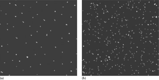
FIGURE 24.9 Two modes of particle image density: (a) low PTV and (b) high PIV.
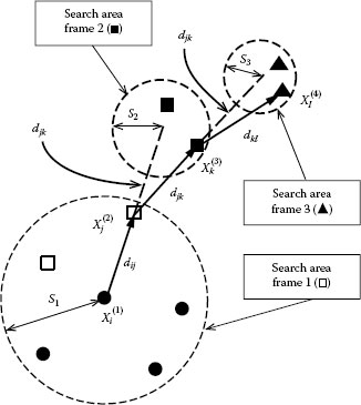
FIGURE 24.10 Schematic diagram of conventional multi-frame PTV tracking algorithm.
When the flow image is of high particle density (Figure 24.9b), the individual particles can be distinguished in each image; however, the displacement pairs of particles during the time interval Δt cannot be identified from the consecutive flow image pairs. In this kind of flow images, each flow image is subdivided into many small interrogation windows and the correlation function of the particle image pair for each interrogation window is numerically calculated. The PIV method extracts the representative velocity vector of each interrogation window from the correlation peak. The cross-correlation PIV algorithm has been widely used for the search of correlation peak due to the merits of nondirectional ambiguity and effectiveness for noise contained flow images. The schematic diagram of the cross-correlation PIV algorithm is represented in Figure 24.11. Nowadays, the PTV and PIV methods are commonly used as a reliable 2D velocity-field measurement technique.
A PIV velocity-field measurement system generally consists of a laser light sheet, an image recording camera, tracer particles, and a computer. Figure 24.12 shows the experimental setup of a PIV system applied on a wind tunnel experiment. The time interval Δt should be chosen a priori in the consideration of free-stream velocity and the magnification of the flow image.
The tracer particles seeded in the flow are assumed to move with the fluid without any velocity lag. This implies that the particles must be small enough to minimize velocity lag due to large particle size and its specific weight should be as close as possible to that of the fluid being measured. For liquid flow, fluorescent, polystyrene, silver-coated particles, or other reflective particles are usually used to seed the flow, while olive oil or alcohol droplets are generally used for wind tunnels tests. Thereafter, tracer particles in the measurement plane of the flow are illuminated by a thin laser light sheet twice with a short time interval Δt. A dual-head Nd:YAG pulse laser is widely used as a laser source. The images of scattered particles in the thin laser light sheet are then captured with a digital CCD or CMOS camera. When the flow images are recorded on a negative film, the chemical development and tedious digitizing procedure with a scanner are required. Finally, the velocity fields of the flow are obtained by digital image processing of the captured flow images.
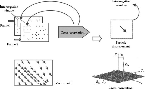
FIGURE 24.11 Schematic of cross-correlation PIV method.
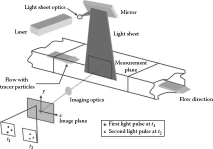
FIGURE 24.12 Schematic for PIV measurement in a wind tunnel.
24.3.4 TYPICAL APPLICATION: MEASUREMENT OF A TURBULENT BOUNDARY LAYER
The PIV velocity-field measurement technique was applied to a turbulent boundary layer formed in a closed return-type wind tunnel. Using the PIV system, 2D in-plane velocity fields (u, v) were measured in the stream-wise-wall-normal (x, y) plane. Olive-oil droplets of 1 μm in mean diameter, generated by a Laskin nozzle, were seeded into the wind tunnel test section as tracer particles. The field of view was illuminated with a thin laser light sheet of approximately 600 μm thickness. The scattered light from tracer particles was captured by a CCD camera of resolution 2048 × 2048 pixels. A delay generator was used to synchronize the laser and camera. The cross-correlation PIV algorithm was applied to the consecutive flow image pairs to calculate instantaneous velocity fields. The size of the interrogation window was 32 × 32 pixels with 50% overlapping. Figure 24.13 shows a typical instantaneous velocity field, subtracted a constant advection velocity from the measured velocity field by using the Galilean decomposition method. The hairpin vortex structures in the turbulent boundary layer are clearly observed as locally swirling vortices in Figure 24.13.
Since most flows of interest are complex 3D turbulent flows, the 2D PIV/PTV techniques were extended to measure the spatial distributions of three velocity components in a plane or a 3D volume. Several SPIV and HPIV methods have been developed as 3D PIV techniques. In addition, micro-PIV technique has been employed to investigate microscale flows such as a flow in a microchannel. They are explained separately in the later parts of this chapter. New PIV/PTV algorithms are still developed worldwide to improve the measurement accuracy and dynamic range. The PIV experiments for 3D turbulent flows should be carried out with care and concern so as to prevent possible sources of error and misinterpretation.
The PIV velocity-field measurement techniques will contribute dominantly to thermo-fluid flow research fields. The PIV data can be compared directly with computational fluid dynamics (CFD) results or theoretical modeling of thermo-fluid flow phenomena.
Most fluid flows encountered in our lives are 3D turbulent flows. Therefore, simultaneous measurement of three orthogonal velocity components is essential for the analysis of 3D flows such as the flow around a fan or propeller. Conventional 2D PIV velocity-field measurement techniques using a single camera provide only in-plane velocity components. The information on the out-of-plane flow motion is embedded in the in-plane flow field data and the out-of-plane velocity component becomes a source of error in the 2D PIV measurements. This implies that most previous studies carried out with a 2D PIV system have perspective errors caused by the out-of-plane velocity component. Figure 24.14 illustrates the perspective error (ΔXp = −Δz × M × tan θ) caused by the out-of-plane displacement (Δz). In the case of constant magnification M, the perspective error is directly proportional to the viewing angle subtended by the particle position at the optical axis of the recording device. The SPIV method can eliminate the perspective error, yielding accurate 3D velocity information in the measurement plane [13].
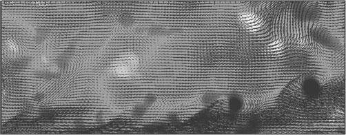
FIGURE 24.13 Instantaneous velocity field of a turbulent boundary layer subtracted by a constant advection velocity.
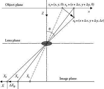
FIGURE 24.14 Perspective error caused by out-of-plane particle motion.
The SPIV techniques usually employ two CCD cameras. Each camera simultaneously captures the same particle displacements at a different angle. The measuring volume is confined by the thickness of the laser light sheet and the imaging area. Two cameras at different angles capture two particle images synchronized with a pulsed laser light sheet. The particle displacements inside the flow images captured by each camera are transposed to 3D velocity-field data by intermediate procedures.
Two stereoscopic configurations have been used for SPIV measurements: the translation configuration and the angular displacement configuration. Different camera arrangements are shown in Figure 24.15. In the translation configuration method, the stereoscopic effects are directly related to the distance between the optical axes of the cameras. The optical axis of the first camera is parallel to the optical axis of the second camera. These optical axes are aligned to be perpendicular to the illuminated plane.
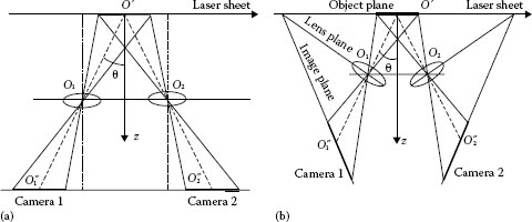
FIGURE 24.15 Different configurations of SPIV system: (a) translation method and (b) angular displacement method.
However, the two optical axes for the angular configuration are neither parallel nor perpendicular to the measurement plane, because the image planes are tilted to focus the whole measuring volume. The tilting of image planes and camera lenses causes image distortion and varying magnification, requiring an elaborate calibration process to obtain accurate flow data. The translation configuration has advantages of convenient mapping and well-focused image over the whole observation area. Since the off-axis aberration restricts the viewing angle, the optical lens was carefully chosen for reducing the off-axis aberration [14].
24.4.2 TYPICAL APPLICATION: FLOW BEHIND AN AXIAL-FAN
The SPIV velocity-field measurement system consists of two CCD cameras with stereoscopic lens, an Nd:YAG pulse laser, and a delay generator. The stereoscopic lenses that were employed have special features for tilting and shifting the lenses without any additional adaptors or stages. They were specially designed to minimize optical aberrations and showed high optical performance throughout the experiments.
SPIV measurements were carried out in a transparent water tank (340 mm × 280 mm × 280 mm). Figure 24.16 shows schematic diagrams of the axial-fan and the field of view for axial plane measurements. The axial-fan tested in this application has five forward-swept blades. The tip-to-tip diameter and hub diameter of the fan are 50 and 14.3 mm, respectively, leading to a hub-to-tip ratio of 0.286. The fan is a 1/10 scale-down model of an outdoor cooling fan used for commercial air conditioners. The axial-fan was installed inside a rectangular basin.
The SPIV system was calibrated using a rectangular calibration target on which white dots were evenly distributed. A translation stage equipped with a micrometer was used to traverse the calibration target aligned with the laser light sheet along the z-direction. The calibration images were captured by two CCD cameras at different z-planes by translating the calibration target along the z-axis. The mapping function F(x) was calculated using a centroid detection algorithm and least square method.
Figure 24.17 represents a typical 3D reconstructed instantaneous velocity field in the measurement plane. During experiments, the fan was rotating at 180 rpm (revolution per minute). The 500 instantaneous velocity fields were measured and they were ensemble averaged to obtain the phase-averaged mean flow structure. By combining the vorticity contours measured at four consecutive phases, isovorticity contours having the same spanwise vorticity (ωz) were derived. The contour plot of the equi-spanwise vorticity surface is depicted in Figure 24.18. It shows the quasi 3D distribution of positive tip vortices shed from the blade tip, trailing vortices, and negative vortices induced from the pressure side of fan blade. The positive tip vortices and negative trailing vortices interact strongly in the region 0.6 < y/R < 0.8.
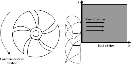
FIGURE 24.16 Schematic diagram of axial-fan and measurement planes.
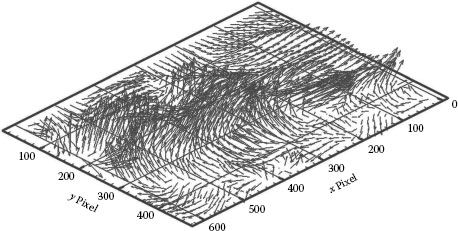
FIGURE 24.17 Typical instantaneous three-component velocity vectors measured by SPIV.
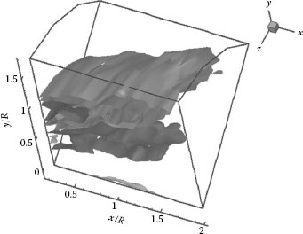
FIGURE 24.18 3D iso-vorticity structure of spanwise vorticity.
24.5.1 FILM-BASED HOLOGRAPHIC PIV
The HPIV method is a 3D velocity-field measurement technique for a whole measurement volume, different from the SPIV method for a measurement plane. However, its practical application to real flows is not easy to apply to real flows because of the complexity of the optical arrangement and experimental setup [15].
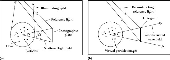
FIGURE 24.19 Off-axis HPIV measurement of tracer particles: (a) recording and (b) reconstruction of the virtual image.
The HPIV measurement has two steps: recording procedure and reconstruction procedure, as shown in Figure 24.19. Like a conventional PIV method, a pulse laser is required for HPIV system to illuminate a test volume. But, the HPIV system differs from conventional method in that it needs holographic film or holographic plate, instead of a CCD camera to record particle images seeded in the test volume. First of all, all particles in the measurement volume are illuminated by an expanded object wave made by passing through a spatial filter. The interference pattern is recorded in a holographic film or plate by the superposition of object wave and reference wave. When the reference and object waves have an oblique angle, it is called an off-axis holography. The coherent length of the laser source should be long enough to form clear interference patterns [16].
The interference pattern, hologram, is used for reconstructing the corresponding virtual particle image. The virtual image is reconstructed by illuminating the hologram with the original reference wave (Figure 24.19b). Since the reconstructed hologram includes the 3D original particle distribution at the initial recoding time, various velocity-field measurement techniques can be applied for a 2D slice selected in the test volume by adjusting the depth of the focusing point of the hologram. The resolution angle in the depth direction depends on the magnitude of the hologram.
Another advantage of the HPIV method is that the real image can be acquired without any lens system. For this real-image acquisition, the hologram should be illuminated by the complex conjugation of reference wave.
In this case, the hologram produces a backward traveling wave, which makes real image of planar laser light. The particle information at any planar section of the test volume can be taken by a CCD camera. The object wave may have optical aberrations due to low-quality windows or optical lens. This distortion would be compensated in the backward traveling path of the conjugated wave. Finally, the original 3D particle image is reconstructed by illuminating the original wave front.
For obtaining high-quality holograms of tracer particles, the wavelength of the laser used for reconstruction should be the same as that of the recording laser, and the geometrical arrangement for the reconstruction procedure should be organized like that of the recording procedure. For example, the wavelength of ruby laser differs from that of He–Ne laser about 10%. This difference can cause disturbance to the complete reconstruction. Therefore, the Nd:YAG pulse laser is much convenient to use due to the presence of a continuous wave (CW) Nd:YAG laser of the same wavelength [17].
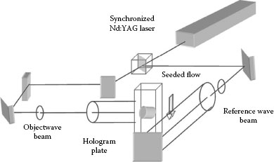
FIGURE 24.20 Schematic of typical holographic installation for PIV recording.
Figure 24.20 shows the schematic diagram of experimental setup for a HPIV experiment. In this figure, an off-axis type reference wave is used for distinguishing the virtual image of particle field from the real image transmitted indirectly. The hologram is brought to completion by double exposure to the same holographic film.
The information of 3D particle location can be obtained by scanning a CCD camera through the reconstructed hologram. Finally, 3D velocity-field information is given by applying the correlation PIV algorithm to the 3D particle information.
In addition to the off-axis HPIV method, many other HPIV methods such as in-line HPIV method, multiple light sheet holography, and hybrid HPIV have been introduced. In the in-line holography, the object and reference waves are overlapped. Compared to a SPIV system, the HPIV technique provides much more flow information, because it measures the 3D velocity components of tracer particles in the whole 3D fluid volume. The film-based HPIV technique has the directional ambiguity problem, when it adopts the single-frame double-exposure method. It also requires cumbersome 3D mechanical scanning and elaborate optical arrangement. Due to the disadvantages and long processing time of the film-based HPIV, the digital HPIV methods have been introduced recently.
24.5.2 DIGITAL HOLOGRAPHIC PTV
The digital holographic PTV (HPTV) technique is basically similar to digital HPIV method, except the procedure to acquire 3D velocity vectors. The basic configuration of digital HPTV system is very simple and similar to conventional 2D PIV systems. A holographic film is replaced by a digital image sensor, eliminating the chemical-processing routine. In other words, the digital holography consists of digital recording and numerical reconstruction procedures. In a film-based HPIV, the off-axis configuration is usually used. However, the digital HPIV does not need to adopt the off-axis configuration, because the directional ambiguity and twin-image problems can be resolved easily using the special intrinsic feature of the digital CCD camera.
Figure 24.21 shows a schematic diagram of the experimental setup for measuring a vertical turbulent jet flow using a digital HPTV technique. The in-line digital HPTV system consists of a CCD camera, a laser, a spatial filter, and a beam expander. He–Ne laser (λ = 632.8 nm) was used as a light source. An AOM (acoustic optical modulator) was used to chop the laser beam into a kind of laser pulse. The hologram images were acquired with a digital CCD camera (PCO SensiCam), which has a spatial resolution of 1280 × 1024 pixels and 12-bit dynamic range. The physical size of each pixel is 6.7 μm. A delay generator was used to synchronize the AOM chopper and CCD camera. For each experimental condition, 100 instantaneous velocity-vector fields were obtained. This single-beam configuration with simple optical arrangement uses the forward scattering method, giving strong light scattering.
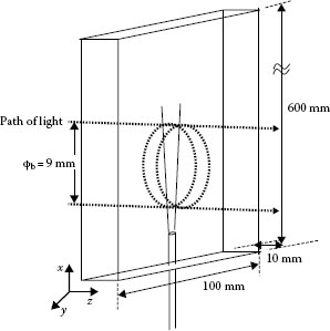
FIGURE 24.21 Experimental setup for HPTV measurement of a jet flow.
Figure 24.22 shows the spatial distributions of tracer particles reconstructed with different particle number density. The number of reconstructed particles (Nr) for the two comparative cases is 671 and 3471, respectively. As shown in Figure 24.22, most of the particles are uniformly distributed. Open circles indicate the particle position in the first frame captured at the first exposure and closed circles denote particle position in the second frame at the second exposure.
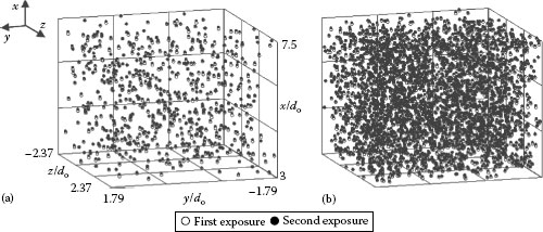
FIGURE 24.22 Distribution of tracer particles reconstructed at different particle concentration Co: (a) Co = 2 (Nr ~ 671) and (b) Co = 13 (Nr ~ 3471).
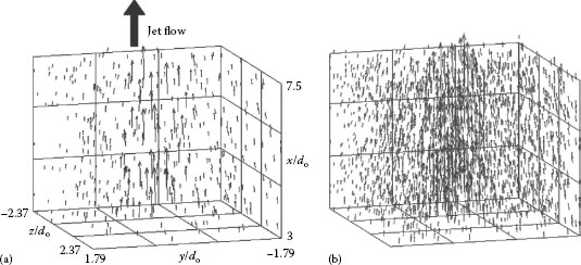
FIGURE 24.23 Instantaneous velocity vectors measured for two different particle concentrations: (a) Co = 2 (Nc ~ 379) and (b) Co = 13 (Nc ~ 2152).
Figure 24.23 shows instantaneous velocity-vector fields measured at the two different particle number densities of Co = 2 and 13 particles/mm3. In case of Co = 13, however, the number of recovered vectors (Nc) is 2152 and the corresponding spatial resolution is about 115 μm. The instantaneous velocity vectors do not show drastic variation in the low-speed flow.
Recently, progress in the bio- and nanotechnology fields has led to heightened interest in the miniaturization and integration of chemical and biological analysis techniques. Work in this area could potentially revolutionize our life style and medical environment through the development of micro-fluidic devices. In fact, many micro-fluidic devices such as biochips, micro-pump, micro-mixer, and micro-heat-exchanger are commercially available already. New researches have been created widely in the field of in micro-fluidics and are receiving large attention nowadays. Such micro-fluidic devices, especially biochips, have various kinds of micro-channels inside. A detailed understanding on the flow inside the micro-channels is essential for the design of the micro-fluidic devices. A micro-PIV system has been employed usefully to measure microscale flow in micro-fluidic devices.
The micro-PIV system consists of an Nd:YAG laser, a CCD camera, a synchronizer, optics, and a computer. Since the field of view is very small, an objective lens of high magnification is usually attached in front of the CCD camera and tracer particles of submicron size are seeded in the flow. In micro-PIV measurements, fluorescent particles of submicron size are commonly used instead of conventional tracer particles because the flow images captured by the volume illumination method suffered from severe light scattering from the channel walls or adjacent peripheral structures. Scattered light can be removed by installing an optical filter in front of the image recorder.
Figure 24.24 shows a schematic diagram of the micro-PIV system used for a typical microchannel experiment. A dual head Nd:YAG laser of wavelength 532 nm illuminates particles seeded inside the micro-channel. The seed particles are fluorescent polystyrene particles of diameter 530 nm that absorb light at λ = 542 nm and emit light at λ = 612 nm. The fluorescent particle images were passed through an optical filter that transmits wavelength longer than 570 nm and then were captured by a cooled CCD camera. As an image recording device, a cooled CCD camera is generally recommended because the light intensity emitted from fluorescent particles is relatively l ow.
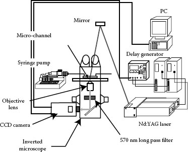
FIGURE 24.24 Experimental setup of micro-PIV system.
This kind of diachronic mirror method has been commonly used for taking fluorescent images from a microscale field of view. In this micro-PIV measurement, a diachronic mirror or emission filter is attached in front of the microscope so that scattered reflection of laser light can be removed effectively and clear fluorescent particle images are usually obtained. The laser beam enters perpendicularly to the micro-channel to excite tracer particles.
As an alternative method, as shown in Figure 24.24, the laser beam directly illuminates the micro-channel from top of the channel by reflecting it with a mirror. Using this method, the image intensity is intensified and light scattering from adjacent structures are removed without any obstacles against the laser beam. Therefore, much clear images can be obtained, compared to the diachronic mirror method.
Figure 24.25 shows the mean stream-wise velocity fields at the entrance region (332 μm × 267 μm) of the six micro-channels having different inlet corner shape. These velocity-field distributions were measured by attaching a 40× objective lens with a numerical aperture of 0.75 in front of the camera. The interrogation window was 48 × 48 pixels in size and 50% overlapped, yielding a spatial resolution of 7.78 μm × 7.78 μm. The mean velocity-field data was obtained by ensemble averaging 80 instantaneous velocity fields. During the experiments, the flow rate supplied by the syringe pump was preset to 1085 μL/h; the corresponding Reynolds number based on the channel hydraulic diameter and mean velocity is about 1.
All PIV measurements were carried out in the mid-depth plane of the channel and the flow direction is from left to right. Figure 24.25 shows that, irrespective of the radius of curvature of the channel inlet corner, the stream-wise mean velocity distribution is almost symmetric with respect to the channel centerline. As the flow enters the channel inlet region, the stream-wise mean velocity is gradually increased. As the radius of curvature of the inlet corner decreases, the stream-wise velocity is noticeably increased in the entrance region and rapidly approaches to a fully developed state. With increasing the radius of curvature of the inlet corner, on the other hand, the flow entering the inlet region becomes smoother and the fully developed stream-wise velocity is increased due to reduction of flow resistance. For the case of r > 0.8w (Figure 24.25e and f), however, the increase of the radius of curvature does not cause noticeable change in the magnitude of the fully developed stream-wise velocity.
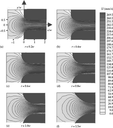
FIGURE 24.25 Stream-wise mean velocity fields of flow in the entrance region of micro-channels having different radius of curvature.
1. Goldstein R.J., 1996, Fluid Mechanics Measurements, 2nd edn., Taylor & Francis, Washington, DC.
2. Guenther R., 1990, Modern Optics, John Wiley & Sons, New York.
3. Adrian R.J., 1991, Particle-imaging techniques for experimental fluid mechanics, Ann. Rev. Fluid Mech., 23: 261–304.
4. Franz M. and Oliver F., 2001, Optical Measurements: Techniques and Applications, Springer-Verlag, New York.
5. Richard S.F. and Donald E.B., 2000, Theory and Design for Mechanical Measurements, Wiley, New York.
6. Choi H.C., Moin P., and Kim J., 1993, Direct numerical simulation of turbulent flow over riblets, J. Fluid Mech., 255: 503–539.
7. Adrian R.J., 1986, Multi-point optical measurements of simultaneous vectors in unsteady flow—A review, Int. J. Heat Fluid Flow, 7: 127–145.
8. Becker R.J., 1999, Particle image velocimetry: A practical guide, M. Raffel et al. (eds.), Appl. Mech. Rev., 52: B42.
9. Gharib M. and Willert C.E., 1990, Particle tracing revisited, in Lecture Notes in Engineering: Advances in Fluid Mechanics Measurements 45, M. Gadel-Hak (ed.), Springer-Verlag, New York, pp. 109–126.
10. Adrian R.J., 1986, Image shifting technique to resolve directional ambiguity in double-pulsed velocimetry, Appl. Opt., 25: 3855–3858.
11. Baek S.J. and Lee S.J., 1996, A new two-frame particle tracking algorithm using match probability, Exp. Fluids, 22: 23–32.
12. Kim H.B. and Lee S.J., 2002, Performance improvement of a two-frame PTV using a hybrid adaptive scheme, Meas. Sci. Technol., 13: 573–584.
13. Arroyo M.P. and Greated C.A., 1991, Stereoscopic particle image velocimetry, Meas. Sci. Technol., 2: 1181–1186.
14. Yoon J.H. and Lee S.J., 2002, Direct comparison of 2-D and 3-D stereoscopic PIV measurement, Meas. Sci. Technol., 13(10): 1631–1642.
15. Barnhart D.H., Adrian R.J., and Papen G.C., 1994, Phase-conjugate holographic system for high-resolution particle image velocimetry, Appl. Opt., 33: 7159–7170.
16. Coupland J.M. and Halliwell N.A., 1992, Particle image velocimetry: Three-dimensional fluid velocity measurements using holographic recording and optical correlation, Appl. Opt., 31: 1005–1007.
17. Zimin V., Meng H., and Hussain F., 1993, Innovative holographic particle velocimeter: A multibeam technique, Opt. Lett., 18: 1101–1103.