chapter 2

Using the Mplus Program

The purpose of this chapter is to introduce you to the general format of the Mplus structural equation modeling (SEM) program so that you can more easily comprehend the applications presented and discussed in Chapters 3 through 12. More specifically, my intent is to (a) familiarize you with the Mplus language used in structuring input files, (b) identify the availability of several analytic and output options, (c) acquaint you with the language generator facility, (d) note important default settings, and (e) alert you to the provision of a graphics module designed for use in displaying observed data and analytic results.

Although Mplus provides for the specification and testing of a broad array of models based on a wide choice of estimators and algorithms for analyses of continuous, categorical (ordinal and nominal), binary (i.e., dichotomous), and censored data, the selection of models illustrated and discussed in this book is necessarily limited only to those considered of most interest to researchers and practitioners wishing to know and understand the basic concepts and applications of SEM analyses. Based on my own experience in conducting close to 100 introductory SEM workshops worldwide, I have found the 10 applications presented in the remaining chapters consistently to have generated the largest number of queries from individuals eager to know more about the rapidly expanding world of SEM. In particular, all models are based on data comprising variables that have either a continuous or an ordinal scale. Readers wishing more specific information related to nominal, censored, or binary data are referred to the Mplus User's Guide (Muthén & Muthén, 2007–2010) and/or website (http://www.statmodel.com).

As with any form of communication, one must first understand the language before being able to interpret the message conveyed. So it is in comprehending the specification of SEM models, as each computer program has its own language and set of rules for structuring an input file that describes the model to be tested. We turn now to this important feature of the Mplus program.

Mplus Notation and Input File Components and Structure

The building of input files using Mplus is relatively easy and straightforward, mainly because its language consists of a maximum of only 10 command statements. As would be expected, however, each of these commands provides for several options that can further refine model specification and desired outcome information. These options notwithstanding, even specification of very complex models requires only minimal input. What makes the structuring of Mplus input files so easy is that in most cases, you will need to use only a small subset of these 10 commands and their options. This minimization of input structure has been made possible largely as a consequence of numerous programmed defaults chosen on the basis of models that are the most commonly tested in practice. Where applicable, these defaults will be brought to your attention; some are noted in this current chapter, and others will be highlighted where applicable in the remaining chapters. It is important for you to know, however, that all programmed defaults can be overridden. Example applications of this option are illustrated in Chapters 5, 9, and 10.

There are several important aspects of these commands and their options that are essential in learning to work with Mplus. Being an inveterate list maker, I always find it most convenient to work from a list when confronted with this type of information. Thus, with the hope of making your foray into the world of SEM a little easier, I now list what I consider to be key characteristics of the Mplus input file. It is important to note, however, that this list is necessarily limited as space considerations weigh heavily on the amount of information I can include here. Thus, for additional and more specific details related to input, readers are referred to the Mplus User's Guide (Muthén & Muthén, 2007–2010).

• Each command must appear on a new line and be followed by a colon.
• With the exception of the TITLE command, information provided for each must always be terminated with a semicolon.
• Command options are separated and terminated by a semicolon.
• There can be more than one option per line of input.
• With the exception of two (to be noted below), a command may or may not be specified.
• Commands can be placed in any order.
• Commands, options, and option settings can be shortened to four or more letters.
• Records comprising the input file can contain upper- and/or lowercase letters and tabs and cannot exceed a length of 90 columns.
• Comments can be included anywhere in the input but must be preceded by an exclamation mark (!); all information that follows is ignored by the program.
• Command options often include the use of keywords critical to appropriate model specification and estimation; these keywords (and one symbol) are IS, ARE, and =, which in most cases can be used interchangeably.

Of the 10 commands, at least four are consistently specified for all applications detailed in this book. Thus, following a description of these four commands, I consider it instructive to stop at that point and show you an example input file before completing descriptions for the remaining commands. Let's turn now to a listing and elaboration of these first four key commands.

TITLE

This command, of course, gives you the opportunity to identify a particular analysis through the creation of a title. In contrast to simply assigning a brief label to the analysis, I strongly recommend that you be generous in the amount of information included in the title. Not uncommon to each of us is the situation where what might have seemed obvious when we conducted the initial analysis of a model may seem not quite so obvious several months later when, for whatever reason, we wish to reexamine the data using the same input files. Liberal use of title information is particularly helpful in the case where numerous Mplus runs were executed for a particular analytic project. Mplus allows you to use as many lines as you wish in this title section.

DATA

This command is always required as it conveys information about the data to the program. Specifically, it provides both the name of the data file and its location in the computer. Of critical note is that the data must be numeric except for certain missing value flags (Muthén & Muthén, 2007–2010) and must reside in an external ASCII file containing not more than 500 variables and with a maximum record length of 5,000. If, for example, your data are in SPSS file format, all you need to do is to save the data as a .dat file. In addition, however, you will need to delete the initial line of data containing all variable names.

In specifying data information, this command typically includes one of the three keywords noted earlier (File IS …). Although there are several options that can be included in this command, three of the most common relate to (a) type of data (e.g., individual, covariance matrix, or correlation matrix), (b) format of data (e.g., free or fixed), and (c) number of observations (or groups, if applicable). If the data comprise individual scores and are of free format, there is no need to specify this optional information as it is already programmed by default. However, if the data are in summary form (i.e., covariance or correlation matrices) the number of observations must be specified (NOBSERVATIONS ARE).

VARIABLE

Consistent with the DATA command, this one too, along with its NAMES option, is always required as it identifies the names of all variables in the data set, as well as which variables are to be included in the analysis (if applicable). Specification of these variables typically includes one of the three keywords noted earlier (e.g., NAMES ARE).

A second important aspect of this command is that all observed data are assumed to be complete (i.e., no missing data) and all observed variables are assumed to be measured on a continuous scale. In other words, these assumptions represent default information. Should this not be the case, then the appropriate information must be entered via a related option statement (e.g., CATEGORICAL ARE).

There are three additional aspects of this command and its options that are worthy of mention here: (a) When the variables in a data file have been entered consecutively, a hyphen can be used to indicate the set of variables to be used in the analysis (e.g., ITEM1—ITEM8); (b) individual words, letters, or numbers in a list can be separated either by blanks or by commas; and (c) a special keyword, ALL, can be used to indicate that all variables are included in the analysis.

MODEL

This command, of course, is always required as it provides for specification of the model to be estimated. In other words, it identifies which parameters are involved in the estimation process. Critical to this process are three essential pieces of information that must be conveyed to the program: (a) whether the variables are observed or unobserved (i.e., latent); (b) whether they serve as independent or dependent (i.e., exogenous or endogenous)¹ variables in the model; and (c) in the case of observed variables, identification of their scale. The latter, as shown earlier, is specified under the VARIABLE command.

Specification of a model is accomplished through the use of three single-word options: BY, ON, and WITH. The BY option is an abbreviation for measured by and is used to define the regression link between an underlying (continuous) latent factor and its related observed indicator variables in, say, a confirmatory factor analysis (CFA) model or measurement model in a full path analytic SEM model. Taken together, the BY option defines the continuous latent variables in the model. The ON option represents the expression regressed on and defines any regression paths in a full SEM model. Finally, the WITH option is short for correlated with. It is used to identify covariance (i.e., correlational) relations between latent variables in either the measurement or structural models; these can include, for example, error covariances.

Despite this textual explanation of these MODEL options, a full appreciation of their specification is likely possible only from inspection and from related explanation of a schematic portrayal of postulated variable relations. To this end, following a description of all Mplus commands, as well as the language generator, I close out this chapter by presenting you with three different very simple models, at which time I walk you through the linkage between each model and its related input file. Thus, how these BY, ON, and WITH options are used should become clarified at that time.

Following description of these first four Mplus commands, let's now review this simple input file:

Turning first to the DATA command, we can see both the name of the data file (FRBDI2.dat) and its location on the computer. Note that this entire string is encased within double quotation marks. Equivalently, we could also have stated this command as follows: File = “C:MplusFiles FRBDI2.dat” (i.e., use of an equal sign [=] in lieu of is). Finally, the fact that there is no mention of either the type or format of data indicates that they comprise individual raw data observations and have a free format.²

Turning next to the VARIABLE command, we see that there is a string of 30 similarly labeled variables ranging from FBD1 through FBD30. However, the next line under this command alerts us that not all 30 variables are to be used in the analysis. As indicated by the Use Variables option, only variables FBD1 through FBD12, plus FBD14, FBD19, and FBD23, will be included.

The MODEL command informs us that Factor 1 will be measured by five indicator variables (FBD8 through FBD12), and Factor 2 measured by three indicator variables (FBD14, FBD19, and FBD23). As such, FBD8 through FBD12 are each regressed onto Factor 1, whereas variables FBD14, FBD19, and FBD23 are regressed onto Factor 2. These regression paths represent the factor loadings of a CFA model or, equivalently, of the measurement model of a full SEM model.

Let's move on to an overview of the remaining Mplus commands, each of which is now described.

DEFINE

The primary purpose of this command is to request transformation of an existing variable and to create new variables. Such operations can be applied to all observed variables or can be limited to only a select group of variables via use of a conditional statement.

ANALYSIS

The major function of this command is to describe technical details of the analysis, which are as follows: type of analysis to be conducted, statistical estimator to be used, parameterization of the model, and specifics of the computational algorithms. Mplus considers four types of analyses— GENERAL, MIXTURE, TWOLEVEL, and EFA. The GENERAL type represents the default analysis; included here are regression analysis, path analysis, CFA, SEM, latent growth curve analysis, discrete-time survival analysis, and continuous-time analysis. Only CFA, SEM, and latent growth curve modeling are included in this book. With respect to statistical estimators, this choice necessarily varies with the particular type of analysis to be conducted. However, for TYPE = GENERAL, maximum likelihood (ML) estimation is default. The PARAMETERIZATION and ALGORITHM options are of no particular concern with the modeling applications to be presented in this book and, thus, are not elaborated upon here.

OUTPUT

The purpose of the OUTPUT command is to request information over and beyond that which is provided by default. Because I include various examples of these OUTPUT options and their related material in all applications presented in this book, I include here only a listing of the usual defaulted output information provided. Accordingly, the default output for all analyses includes a record of the input file, along with summaries of both the analytic specifications and analytic results. This information will be detailed for the first application (Chapter 3) and additionally inspected and reported for all subsequent applications in the book.

The initial information provided in the Mplus output file represents a replication of the input file. This repeated listing of the command statements can be extremely helpful, particularly in the face of unexpected results, as it enables you to double-check your specification commands pertinent to the model under study.

The next set of information in the output file is a summary of the analytic specifications. The importance of this section is that it enables you to see how the program interpreted your instructions regarding the reading of data and requested analytic procedures. In particular, it is essential to note here whether or not the reported number of observations is correct. Finally, in the event that Mplus encountered difficulties with your input instructions and/or the data file, any warnings or error messages generated by the program will appear in this section of the output. Thus, it is important to always check out any such messages as they will be critical to you for resolving the analytic roadblock.

The third and final block of Mplus output information, by default, summarizes results of the analysis conducted. Here we find (a) the model goodness-of-fit results, (b) the parameter estimates, (c) the standard errors, and (d) parameter significance test results as represented by a ratio of the parameter estimate divided by its standard error (referred to in other programs as t-values [LISREL], z-values [EQS], and C.R. [critical ratio] values [AMOS]. As noted earlier, examination and discussion of these defaulted output components will accompany all applications in this book, and thus further elaboration is not detailed here.

SAVEDATA

The primary function of this command is to enable the user to save a variety of information to separate files that can be used in subsequent analyses. In general terms, this command allows for the saving of analytic data, auxiliary variables, and a range of analytic results. Three common and popular examples include the saving of matrix data (correlation, covariance), factor scores, and outliers. Readers are referred to the Mplus User's Guide (Muthén & Muthén, 2007–2010) for a perusal of additional options.

PLOT

Inclusion of this command in the input file requests the graphical display of observed data and analytic results. These visual presentations can be inspected after the analysis is completed using a dialog-based postprocessing graphics module. Although a few of these graphical displays will be presented with various applications in this book, a brief description of the PLOT options is provided here.

The PLOT command has three primary options: TYPE, SERIES, and OUTLIERS. There are three types of plots, labeled as PLOT1, PLOT2, and PLOT3, each of which produces a different set of graphical displays. Thus, specification of the TYPE option allows the user to select a plot pertinent to a particular aspect of his or her data and/or analytic results.

The SERIES option allows for the listing of names related to a set of variables to be used in plots in which the values are connected by a line. This specification also requires that the x-axis values for each variable be provided. Of important note is that non–series plots (e.g., histograms and scatterplots) are available for all analyses.

Finally, the OUTLIERS option is specified when the user wishes to select and save outliers for use in graphical displays. Accordingly, Mplus provides the choice of four methods by which outliers are identified: the Mahalanobis distance plus its p-value (MAHALANOBIS), Cook's D parameter estimate influence measure (COOKS), the loglikelihood contribution (LOGLIKELIHOOD), and the loglikelihood distance influence measure (INFLUENCE).

MONTECARLO

As is evident from its label, the MONTECARLO command is used for the purposes of specifying and conducting a Monte Carlo simulation study. Mplus has extensive Monte Carlo capabilities used for data generation as well as data analysis. However, given that no Monte Carlo analyses are illustrated in this introductory book, no further information will be presented on this topic.

Having reviewed the 10 possible commands that constitute the major building blocks of Mplus input files, along with some of the many options associated with these commands, let's move on now to the Mplus language generator.

The Mplus Language Generator

The language generator is a very helpful feature of the Mplus program as it makes the building of input files very easy. Not only does it reduce the time involved in structuring the file, but also it ensures the correct formulation of all commands and their options. The language generator functions by taking users through a series of screens that prompt for related information pertinent to their data and analyses. However, one caveat worthy of note is that this facility contains all Mplus commands except for DEFINE, MODEL, PLOT, and MONTECARLO.

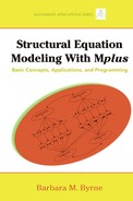
Let's now review Figures 2.1 and 2.2, where we can see how easy it is to work with the language generator in structuring an Mplus input file.³ Turning first to Figure 2.1, note that once you click on the Mplus tab, this action opens a dialog box containing the language generator. By clicking on the latter option, as shown in Figure 2.2, you are then presented with a list of choices from which to select the correct type of analysis for the model under study. In Chapter 3, we will proceed through the steps that necessarily follow, at which time I walk you through this automated file-building process as it pertains to the first application of this book. Thus, further details related to the language generator will be presented at that time.

Figure 2.1. Selecting the Mplus language generator.

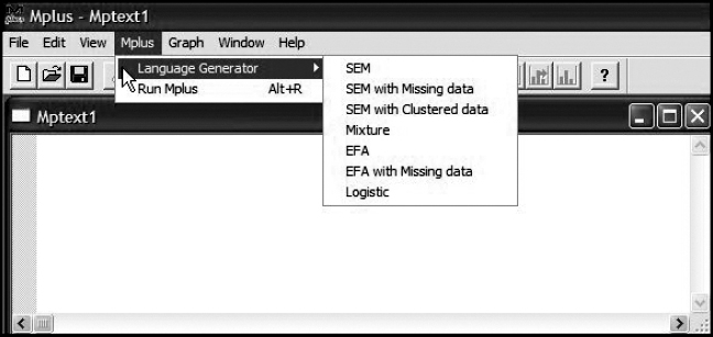
Figure 2.2. The Mplus language generator menu options.

Model Specification From Two Perspectives

Newcomers to SEM methodology often experience difficulty in making the link between specification of a model as documented in a programmed input file and as presented in a related graphical schema. In my experience, I have always found it easiest to work from the schematic model to the input file. In other words, translate what you see in the model into the command language of the SEM program with which you are working. To help you in developing an understanding of the link between these two forms of model specification, I now walk you through the specification of three simple, albeit diverse model examples: (a) a first-order CFA model (Figure 2.3), (b) a second-order CFA model (Figure 2.4), and (c) a full SEM model (Figure 2.5).

Example 1: A First-Order CFA Model

In reviewing Figure 2.3, we observe a model that is hypothesized to have four factors—Sense of Humor (Factor 1), Trustworthiness (Factor 2), Sociability (Factor 3), and Emotional Stability (Factor 4). Let's say that these factors represent four subscales of an instrument designed to measure Social Acceptance. As indicated by the configuration of the 16 rectangles, each factor is measured by four observed (indicator) variables, which in this case represent items comprising the assessment scale: Items 1–4 measure Factor 1, Items 5–8 measure Factor 2, Items 9–12 measure Factor 3, and Items 13–16 measure Factor 4. The double-headed arrows linking the four factors indicate their postulated intercorrelation; the single-headed arrows leading from each factor to its related indicator variables represent the regression of this set of item scores onto their underlying constructs (i.e., the factor loadings); and the single-headed arrows pointing to each of the observed variables represent measurement error. Recall, however, that these errors are termed residuals in Mplus.

Although this review of the model thus far should seem somewhat familiar to you, there are two features that are worthy of some elaboration. The first of these relates to the double labeling of each indicator variable shown in the model. Recall from Chapter 1 that Mplus notation designates outcome continuous variables as y. For purposes of clarification in helping you understand the rationale for this labeling, I have assigned a y label to each indicator variable, in addition to its more general variable label.⁴ We can think of the item scores as representing outcome variables as they are influenced by both their underlying latent factor and measurement error. Another way of thinking about them is as dependent variables. In SEM, all variables, regardless of whether they are observed or latent, are either dependent or independent variables in the model. An easy way of determining this designation is as follows: Any variable having a single-headed arrow pointing at it represents a dependent variable in the model; otherwise, it is an independent variable in the model. As is evident from the model shown in Figure 2.3, all of the observed item scores have two arrows pointing at them, thereby indicating that they are dependent variables in the model.

The second important point relates to the “1’s” (shown here within callouts) assigned to the first factor loading in each set of factor loadings. These 1’s represent fixed parameters in the model. That is to say, the factor loadings to which they are assigned are not freely estimated; rather, they remain fixed to a value of 1.0.⁵ There are at least three important points to be made here. First, the value assigned to these parameters need not be 1.0. Although any numeral may be assigned to these parameters, a value of 1.0 typically has been the assignment of choice. Second, the constrained parameter need not be limited to the first indicator variable; any one of a congeneric⁶ set of parameters may be chosen. Finally, over and above these technical notations, however, there are two critically important points to be made regarding these fixed factor loadings: They address the issues of (a) model identification (also termed statistical identification) and (b) latent variable scaling, topics to which we turn shortly.

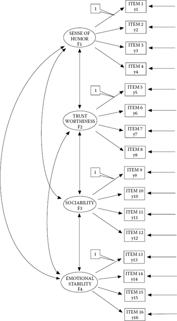
Figure 2.3. Hypothesized first-order CFA model.

Critical to knowing whether or not a model is statistically identified is your understanding of the number of estimable parameters in the model. Thus, one extremely important caveat in working with structural equation models is to always tally the number of freely estimated parameters prior to running the analyses. As a prerequisite to the discussion of model identification, then, let's count the number of parameters to be estimated for the model portrayed in Figure 2.3. From a review of this figure, we ascertain that there are 16 regression coefficients (factor loadings), 20 variances (16 error variances and 4 factor variances), and 6 factor covariances. The 1’s assigned to one of each set of the regression path parameters represent a fixed value of 1.00; as such, these parameters are not estimated. In total, then, there are 38 parameters to be estimated for the CFA model depicted in Figure 2.3; these are 12 factor loadings, 16 error variances, 4 factor variances, and 6 factor covariances. By default, however, Mplus also estimates the observed variable intercepts, thereby making the number of parameters estimated to be 54 (38 + 16).

Before addressing the issues of model identification and latent variable scaling, let's first review the Mplus input file pertinent to this CFA model:

As is evident from this file, the amount of text input is minimal. Three important aspects of this file are worthy of note. First, given that (a) the data file comprises only 16 variables (ITEM1–ITEM16), (b) the variables have been entered into the data file consecutively beginning with ITEM1, and (c) all variables are used in the analysis, there is no need to include the option USE VARIABLES. Second, the MODEL command provides for information that defines how the observed variables load onto each of the four factors; in other words, which observed variable measures which factor. This information is conveyed through use of the word by. A review of each option comprising the word by indicates that F1 is to be measured by the variables ITEM1 through ITEM4, F2 by ITEM5 through ITEM8, F3 by ITEM9 through ITEM12, and F4 by ITEM13 through ITEM16. Finally, three important programmed defaults come into play in this model: (a) As noted earlier, by default, Mplus fixes the first factor loading in each congeneric set of indicator variables to 1.0 in CFA models and/or the measurement portion of other SEM models, (b) variances of and covariances among independent latent variables (i.e., the variances of F1–F4) are freely estimated,⁷ and (c) residual variances of dependent observed variables (i.e., the error variances associated with each observed variable) are freely estimated. Due to defaults (b) and (c) noted here, no specifications for these parameters are needed, and therefore are not shown in the input file related to the CFA model in Figure 2.3.

That Mplus makes no distinction in terminology between factor variance and residual variance can be confusing for new users. Furthermore, the fact that they are both estimated by default for continuous variables (as in this case) may exacerbate the situation. Thus, I consider it important to both clarify and emphasize the approach taken in this regard. Specifically, Mplus distinguishes between these two types of variance based on their function in the model; that is, in terms of whether the variance parameter is associated with an independent or dependent variable in the model. If the former (i.e., there are no single-headed arrows pointing at it), then Mplus considers the parameter to represent a factor variance. If, on the other hand, the parameter is associated with a dependent variable in the model (i.e., there is a single-headed arrow pointing at it), then Mplus interprets the variance as representing residual variance. In short, factor variances are estimated for independent variables, whereas residual variances are estimated for dependent variables (see note 3).

Now that you have made the link in model specification between the graphical presentation of the model and its related program input file, let's return to a brief discussion of the two important concepts of model identification and latent variable scaling.

The Concept of Model Identification

Model identification is a complex topic that is difficult to explain in nontechnical terms. Although a thorough explanation of the identification principle exceeds the scope of the present book, it is not critical to the reader's understanding and use of the book. Nonetheless, because some insight into the general concept of the identification issue will undoubtedly help you to better understand why, for example, particular parameters are specified as having certain fixed values, I attempt now to give you a brief, nonmathematical explanation of the basic idea underlying this concept. However, I strongly encourage you to expand your knowledge of the topic via at least one or two of the following references. For a very clear and readable description of issues underlying the concept of model identification, I highly recommend the book chapter by MacCallum (1995) and monographs by Long (1983a, 1983b). For a more comprehensive treatment of the topic, I refer you to the following texts: Bollen (1989), Brown (2006), Kline (2011), and Little (in press). Finally, for an easy-to-read didactic overview of identification issues related mostly to exploratory factor analysis, see Hayashi and Marcoulides (2006); and for a more mathematical discussion pertinent to specific rules of identification, see Bollen and Davis (2009).

In broad terms, the issue of identification focuses on whether or not there is a unique set of parameters consistent with the data. This question bears directly on the transposition of the variance–covariance matrix of observed variables (the data) into the structural parameters of the model under study. If a unique solution for the values of the structural parameters can be found, the model is considered identified. As a consequence, the parameters are considered to be estimable, and the model therefore testable. If, on the other hand, a model cannot be identified, it indicates that the parameters are subject to arbitrariness, thereby implying that different parameter values define the same model; such being the case, attainment of consistent estimates for all parameters is not possible, and, thus, the model cannot be evaluated empirically. By way of a simple example, the process would be conceptually akin to trying to determine unique values for X and Y, when the only information you have is that X + Y = 15. Generalizing this example to covariance structure analysis, then, the model identification issue focuses on the extent to which a unique set of values can be inferred for the unknown parameters from a given covariance matrix of analyzed variables that is reproduced by the model.

Structural models may be just identified, overidentified, or underidentified. A just-identified model is one in which there is a one-to-one correspondence between the data and the structural parameters. That is to say, the number of data variances and covariances equals the number of parameters to be estimated. However, despite the capability of the model to yield a unique solution for all parameters, the just-identified model is not scientifically interesting because it has no degrees of freedom and therefore can never be rejected. An overidentified model is one in which the number of estimable parameters is less than the number of data points (i.e., variances and covariances of the observed variables). This situation results in positive degrees of freedom that allow for rejection of the model, thereby rendering it of scientific use. The aim in SEM, then, is to specify a model such that it meets the criterion of overidentification. Finally, an underidentified model is one in which the number of parameters to be estimated exceeds the number of variances and covariances (i.e., data points). As such, the model contains insufficient information (from the input data) for the purpose of attaining a determinate solution of parameter estimation; that is, an infinite number of solutions are possible for an underidentified model.

Reviewing the CFA model in Figure 2.3, let's now determine how many data points we have to work with (i.e., how much information do we have with respect to our data?). As noted above, these constitute the variances and covariances of the observed variables. Let's say we have p variables with which to work; the number of elements comprising the variance–covariance matrix will be p (p + 1) / 2. Given that there are 16 observed variables shown in Figure 2.3, this means that we have 16 (16 + 1) / 2 = 136 data points. In addition, however, because Mplus estimates the observed variable intercepts by default, the observed means also contribute to information upon which the analysis is based. Pertinent to this example, then, we add 16 means to this total, thereby giving us 152 (136 + 16) data points. Prior to this discussion of identification, we determined a total of 54 unknown parameters (including the intercepts). Thus, with 152 data points and 54 parameters to be estimated, we have an overidentified model with 98 degrees of freedom.

It is important to point out, however, that the specification of an overidentified model is a necessary but not sufficient condition to resolve the identification problem. Indeed, the imposition of constraints on particular parameters can sometimes be beneficial in helping the researcher to attain an overidentified model. An example of such a constraint is illustrated in Chapter 5 with the application of a second-order CFA model.

The Concept of Latent Variable Scaling

Linked to the issue of identification is the requirement that every latent variable have its scale determined. This requirement arises because latent variables are unobserved and therefore have no definite metric scale; this requirement can be accomplished in one of three ways. The first and most commonly applied approach is termed the reference variable method. This approach is tied to specification of the measurement model whereby the unmeasured latent variable is mapped onto its related observed indicator variable. This scaling requisite is satisfied by constraining to some nonzero value (typically 1.0), one factor-loading parameter in each congeneric set of loadings. This constraint holds for both independent and dependent latent variables in a model. In reviewing Figure 2.3, this means that, for one of the three regression paths leading from each Social Acceptance factor to a set of observed indicators, some fixed value should be specified; this fixed parameter is termed a reference variable (or reference indicator). With respect to the model in Figure 2.3, for example, the scale has been established by constraining to a value of 1.0, the first parameter in each congeneric set of observed variables. Thus, there is no need to specify this constraint in the input file. However, should you wish instead to constrain another factor loading within the same congeneric set as the reference variable, the specified constraint would need to be included in the input file. This alternate specification is demonstrated in Chapters 5 and 10.

The second approach to establishing scale for latent variables is termed the fixed factor method. Using this procedure of scaling, the factor variances are constrained to 1.0. Should this be the preferred approach, then all factor loadings are freely estimated. These first two scale-setting approaches have generated some debate in the literature regarding the advantages and disadvantages of each (see, e.g., Gonzalez & Griffin, 2001; Little, Slegers, & Card, 2006). More recently, however, Little et al. (2006) have proposed a third approach, which they term the “effects coding” method. These authors posited that, of the three approaches, the latter is the only scale-setting constraint that both is nonarbitrary and provides a real scale. Regardless of the reported pros and cons related to these three scale-setting approaches, the reference variable method, at this point in time, is the procedure most widely used (Brown, 2006).

Now that you have a better idea of important aspects of the specification of a CFA model in general, specification using the Mplus program in particular, and the basic notions associated with model identification and latent variable scaling, let's move on to inspect the remaining two models to be reviewed in this chapter.

Example 2: A Second-Order CFA Model

This second example model, shown in Figure 2.4, supports the notion that one's sense of humor, trustworthiness, sociability, and emotional stability are influenced by some higher order global construct, which we might term self-perceived social competence. Thus, although the first-order structure of this model remains basically the same as in Figure 2.3, there are four important differential features that need to be noted. First, in contrast to the first-order CFA example in which only regression paths between the observed variables and their related underlying factors are specified, this second-order model also includes regression paths between these first-order factors and the higher order factor. Specifically, these parameters represent the impact of F5 (an independent variable in the model) on F1, F2, F3, and F4. Second, consistent with the first-order CFA structure, whereby one factor loading from each congeneric set of indicator variables was constrained to 1.0 for purposes of model identification and latent variable scaling, so too this concern needs to be addressed at the higher order level. Once again, by default, Mplus automatically fixes the value of the first higher order factor loading to a value of 1.0, as shown in the callout in Figure 2.4. More typically, however, researchers tend to fix the variance of the higher order factor to 1.0, rather than one of the higher order loadings, as estimation of the factor loadings is of more interest. Again, this alternate specification is demonstrated in Chapter 5. Third, given that SELF-PERCEIVED SOCIAL COMPETENCE is hypothesized to cause each of the four first-order factors, F1 through F4 now represent dependent variables in the model. Accordingly, SENSE OF HUMOR, TRUSTWORTHINESS, SOCIABILITY, and EMOTIONAL STABILITY are hypothesized as being predicted from self-perceived social competence, but with some degree of error, which is captured by the residual term, as indicated in Figure 2.4 by the single-headed arrow pointing toward each of these four factors. Finally, in second-order models, any covariance among the first-order factors is presumed to be explained by the higher order factor(s). Thus, note the absence of double-headed arrows linking the four first-order factors in the path diagram.

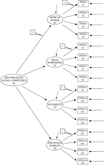
Figure 2.4. Hypothesized second-order CFA model.

Turning now to the Mplus input file pertinent to this higher order model, the only difference between this specification and the one for the first-order CFA model is the added statement of “F5 by F1–F4.” This statement, of course, indicates that F1 through F4 are regressed onto the higher order factor, F5. Importantly, with one exception, the Mplus defaults noted for Figure 2.3 also hold for Figure 2.4. The one differing default relates to the factor variances for F1 through F4, which now are not estimated. More specifically, given that in this second-order model, F5 (Social Competence) is postulated to “cause” the first-order factors (F1–F4), these four factors are now dependent variables in the model. As a consequence, this specification triggers Mplus to estimate their residuals by default, thereby negating any need to include their specification in the input file.

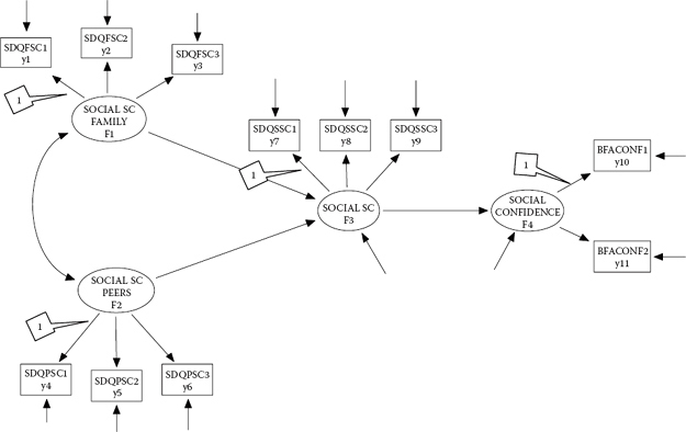
Figure 2.5. Hypothesized full structural equation model.

Example 3: A Full Structural Equation Model

The path diagram shown in Figure 2.5, considered within the context of an adolescent population, postulates that one's social self-concept (SC), in general, is influenced by two more specific-type SCs: social SC as it relates to the family and social SC as it relates to peers. (General) social SC, in turn, is postulated to predict one's sense of social confidence. In reviewing this full SEM model, shown in Figure 2.5, I wish to draw your attention to three particular specifications. First, note that, of the four factors comprising this model, only F1 and F2 are independent variables in the model (i.e., they have no single-headed arrows pointing at them); all other factors operate as dependent variables in the model. Thus, only the variances for F1 and F2, together with their covariance (indicated by the double-headed arrow), are freely estimated parameters in the model. Second, as with the second-order model shown in Figure 2.4, here again we have regression equations involving two factors. In the present case, equations are specified for F3 and F4 only, as each is explained by other factors in the model. More specifically, F1 and F2 are hypothesized to predict F3, which in turn predicts F4. Third, given the dependent variable status of F3 and F4 in the model, note the presence of their residual variances, represented by the short single-headed arrows pointing toward each of these factors. Finally, it is worth noting that, although Factor 3 would appear to operate as both an independent and a dependent variable in the model, this is not so. Once a variable is defined as a dependent variable in a model, it maintains that designation throughout all analyses bearing on the hypothesized model.

Let's look now at this final example of an Mplus input file:

Three aspects of this input file are worthy of elaboration here. First, turning to the MODEL command, we look first at the measurement portion of the model. Accordingly, “F1 by SDOFSC1–SDQFSC3” indicates that F1 is measured by three observed variables—SDQFSC1 through SDQFSC3; likewise, this pattern follows for the next three specifications, albeit F4 is measured by only two observed measures. Third, the structural portion of the model is described by the last two lines of input. The specification “F4 on F3” states that F4 is regressed on F3; likewise, the statement “F3 on F1, F2” advises that F3 is regressed on both F1 and F2. Finally, the defaults noted earlier for the other two models likewise hold for this full SEM model. That is, (a) the first factor loading of each congeneric set of indicator variables is constrained to 1.0, (b) the factor variances for F1 and F2 are freely estimated, (c) the factor covariance between F1 and F2 is freely estimated, (d) residual variances associated with the observed variables are freely estimated, and (e) residual variances associated with F3 and F4 are freely estimated. Thus, specification regarding these parameters is not included in the input file.

Overview of Remaining Chapters

Thus far, I have introduced you to the bricks and mortar of SEM applications using the Mplus program. As such, you have learned the basics regarding the (a) concepts underlying SEM procedures, (b) components of the CFA and full SEM models, (c) elements and structure of the Mplus program, (d) creation of Mplus input files, and (e) major program defaults related to the estimation of parameters. Now it's time to see how these bricks and mortar can be combined to build a variety of other SEM models. The remainder of this book, then, is directed toward helping you understand the application and interpretation of a variety of CFA and full SEM models using the Mplus program.

In presenting these applications from the literature, I have tried to address the diverse needs of my readers by including a potpourri of basic models and Mplus setups. All data related to these applications are included at the publisher's website http://www.psypress.com/sem-with-mplus. Given that personal experience is always the best teacher, I encourage you to work through these applications on your own computer. Taken together, the applications presented in the next 10 chapters should provide you with a comprehensive understanding of how Mplus can be used to analyze a variety of structural equation models. Let's move on, then, to the remaining chapters, where we explore the analytic processes involved in SEM using Mplus.

Notes

1.	The terms independent and dependent will be used throughout the remainder of the book.
2.	Importantly, if the data file resides in the same folder as the input file(s) for which it will be used, it is not necessary to specify the path string.
3.	It is important to note that in order to activate the language generator, you must first indicate to the program that you are creating a new file. This is accomplished by clicking on the “FILE” tab and selecting the “NEW” option.
4.	The labeling of y1, of course, presumes that it is the first variable in the data set. If, on the other hand, it had been the fifth variable in the data set, it would rightfully be labeled y5.
5.	In Mplus, these parameters are automatically fixed to 1.0 by default. That is, if you intend the first factor loading in each set to be fixed to 1.0, there is no need to specify this constraint.
6.	A set of measures is said to be congeneric if each measure in the set purports to assess the same construct, except for errors of measurement (Jöreskog, 1971a). For example, as indicated in Figure 2.3, ITEM1, ITEM2, ITEM3, and ITEM4 all serve as measures of the factor SENSE OF HUMOR; they therefore represent a congeneric set of indicator variables.
7.	An important tenet in SEM is that variances and covariances of only independent variables in the model (in the SEM sense) are eligible to be freely estimated.