
chapter 12
Testing Within- and
Between-Level Variability
The Multilevel Model
In contrast to the multigroup models illustrated in Chapters 7, 8, and 9 in which analyses were based on data representing different populations, the multigroup model examined in this chapter focuses on a single population that is hierarchically structured. Such models are termed multilevel (MLV) models because the data lend themselves to more than one level of analyses. Most commonly, examples of hierarchically structured data are (a) students nested within schools, (b) patients nested within clinics, (c) employees nested within firms or corporations, and (d) children and adults nested within families, among others. Such hierarchical structures are often termed nested data or clustered data. In essence, however, hierarchical structures may involve more than two levels of analysis. For example, building upon these earlier examples, data could be extended to include schools nested within districts, and districts nested within states; or employees nested within departments, departments nested within business organizations, organizations nested within regions, and so on.
Beyond these examples, however, substantial methodological research over this past decade has shown that hierarchical structures can be studied from a wide variety of perspectives. Although this work clearly exceeds the scope of the present volume, I highly recommend that you review at least a few of these intriguing, albeit ever-growing applications of MLV modeling within the framework of structural equation modeling (SEM).1 For readers interested in longitudinal analyses in general, and/or latent growth curve modeling in particular, see Baumler, Harrist, and Carvajal (2003); Chen, Kwok, Luo, and Willson (2010); Chou, Bentler, and Pentz (2000); Ecob and Der (2003); Heck and Thomas (2009); Hoffman (2007); Hox (2000, 2002, 2010); Hung (2010); Jo and Muthén (2003); Kaplan, Kim, and Kim (2009); Kwok, West, and Green (2007); Little, Schnabel, and Baumert (2000); MacCallum and Kim (2000); and Muthén, Khoo, Francis, and Boscardin (2003). More recently, enormous progress has been made in advancing MLV modeling applications to numerous other areas of research. Suggested publications on these specific topics are as follows: multitrait—multimethod analyses (Hox & Kleiboer, 2007), mediation analyses (Preacher, Zyphur, & Zhang, 2010), item response theory analyses (Hsieh, von Eye, & Maier, 2010), and meta-analyses (Hox, 2010; Hox & de Leeuw, 2003). Finally, other MLV modeling issues capturing the interests of methodological researchers have focused on use of categorical data (see Fielding, 2003; Heck & Thomas, 2009; Hox, 2010; Hung, 2010; Kaplan et al., 2009), determination of reliability (Raykov & Penev, 2010), and specification searches (Peugh & Enders, 2010).
The application illustrated in the present chapter represents a two level analysis (CFA) model based on item responses to the Family Values (FV) Scale (Georgas, 1999) for 5,482 university students (2,070 males and 3,160 females) from 27 countries; gender scores were missing for Germany (n = 7), India (n = 1), Mexico (n = 1), Nigeria (n = 3), Ukraine (n = 1), and Indonesia (n = 239).2 The example presented here extends the work of Byrne and van de Vijver (2010) that probed the many complexities associated with testing for measurement invariance across diverse cultural groups. (For details related to sample size, gender composition, and mean age by country, see Byrne & van de Vijver, 2010.)
Overview of Multilevel Modeling
As noted by Selig, Card, and Little (2008), in general terms, “[A]ny model that can be depicted as a multigroup SEM, can also be defined as a multilevel SEM, given that the data are hierarchically clustered as individuals within groups” (p. 102). In its simplest form, the data are represented by a two-level structure, with the lower level representing individuals (e.g., students and employees) and the upper level representing groups (e.g., schools and companies). Taken together, the primary objective of MLV modeling is to summarize within-group variability at the individual (or lower) level and between-group variability at the group (or higher) level. These levels are often referred to as Level 1 and Level 2, respectively.
Over this past decade, MLV modeling has been increasingly recognized as one of the most effective means to investigating hierarchical data. Until relatively recently, however, practical application of MLV modeling has tended to lag behind the substantive theory to which it is grounded. This delay in the use of MLV modeling can be linked to the inability of earlier SEM software packages to adequately address complexities such as the computation of separate covariance matrices for sampling units of varying sample sizes and the provision of appropriate estimators (Heck & Thomas, 2009; Hox, 2002; McArdle & Hamagami, 1996). As a consequence, researchers working with hierarchical data had no choice but to disregard the rich source of potential information provided by such data, thereby limiting their investigation to single-level analyses either on the lowest level of measurement (e.g., students) or on the highest level of measurement (e.g., schools). Rephrased differently, researchers needed either to disaggregate or to aggregate variables from their nested data in order to enable single-level analyses (Heck, 2001). Importantly, however, when such hierarchical structure is ignored, problematic repercussions necessarily occur at both the individual (i.e., disaggregated) and group (i.e., aggregated) levels, thereby leading to several analytic and interpretation difficulties, a topic to which we now turn.
Single-Level Analyses of Hierarchical Data: Related Problems
The Disaggregation Approach
In using this approach, analyses focus on the individual (or lower) level of the hierarchy and necessarily lead to violation of two major statistical assumptions: (a) that all observations are independent, and (b) that all random errors are independent, normally distributed, and homoscedastic. Violation of the first assumption implies that all individuals within similar organizational or societal units share no common characteristics, which of course is totally unreasonable (Heck, 2001; Julian, 2001). Indeed, Muthén and Satorra (1995) reported that the more pronounced the similarities among individuals within groups, the more biased will be the parameter estimates, standard errors, and related tests for significance. Violation of the second assumption, on the other hand, suggests no systematic influence of variables at the higher level, which again is erroneous and unrealistic (Kreft & de Leeuw, 1998). Taken as a whole, disregard for hierarchical structure of the data has the potential to yield underestimated standard errors and, as a result, an inflated Type I error rate (Bovaird, 2007).
The Aggregated Approach
In like manner, single-level analyses of data that focus on the group (or higher) level are equally problematic. As such, the groups (e.g., schools) form the unit of analysis with the individual data used to develop mean scores on the variables as they relate to each organization (Heck, 2001). Again, there are at least three limitations associated with these higher level analyses: (a) Given that all variability within each organizational unit is reduced to a single mean, any differences found at the group level will appear stronger than would be the case if within-organizational (i.e., individual) variability were also incorporated into the analysis (Kaplan & Elliott, 1997);3 (b) in situations where the individual-level data for particular variables (e.g., socioeconomic status) may be scant in some groups, the attainment of efficient estimates is made more difficult, thereby resulting in less efficient prediction equations for these groups (Bryk & Raudenbush, 1992); and (c) aggregated analyses can lead to reduced statistical power, inaccurate representations of group-level relations, and increased risk of incorrectly drawing causal inferences from individual-level behavior based on group-level data (Bovaird, 2007). Given substantial focus on cross-cultural mean comparisons, this latter point, termed the ecological fallacy (Robinson, 1950), remains one of the most notable problems associated with cross-cultural research.
Multilevel Analyses of Hierarchical Data
In contrast to single-level analyses, MLV modeling allows the researcher to consider both levels of the hierarchically structured data simultaneously. In particular, it enables the partitioning of total variance into within- and between-group components and allows a separate structural model to be specified at each level. For example, in the case of students nested within schools, this would mean that the total covariance matrix, Σ, is partitioned into a within-covariance matrix (ΣW) and a between-covariance matrix (ΣB. The ΣW matrix represents covariation at the individual level (i.e., individual differences in, say, math self-concept) and their correlates, albeit controlling for variation across schools. In contrast, the ΣB matrix represents covariation at the school level (i.e., differences across schools in, say, school climate) and their correlates. The ΣW and ΣB covariance matrices may have similar or totally different model structures. For each student, then, the total score is decomposed into an individual component (i.e., individual deviation from the group mean) and a group component (i.e., the disaggregated school group mean). It is via this individual decomposition that the separate within- and between-group covariance matrices are computed (Heck, 2001; Hox, 2002). Not surprisingly, the related effects are termed within-cluster and between-cluster effects (see Bentler, 2005). If a mean structure is needed, it is used to model the between-group means.
As an aid to conceptualizing the MLV model, McArdle and Hamagami (1996) suggested that one think of it as a typical multisample analysis. The rationale underlying this proposal stems from the fact that analyses focus on the estimation of two unstructured matrices, ΣW and each of which represents a separate model. Although the standard statistical assumption of independent groups, of course, cannot be made, such a model can nonetheless be thought of as a two-group multigroup model (Bentler, 2005).
MLV Model Estimation
In the early years of MLV modeling within the framework of SEM, analytic approaches to the estimation of parameters involved mainly full information maximum likelihood (FIML; hereafter shortened to maximum likelihood [ML]) estimation and Muthén's (1994) approximate maximum likelihood (MUML) estimation. Whereas ML estimation demanded that group sizes be balanced (i.e., into clusters of equal size), MUML estimation represented a limited ML method of analyses that allowed for unbalanced groups (i.e., with clusters of unequal sizes). More specifically, whereas ML estimation based on data representing unbalanced groups yielded incorrect χ2 values, fit indices, and standard errors (Kaplan, 1998; Muthén, 1994), the MUML estimator did not exhibit this limitation. On the other hand, when used with balanced groups, the MUML estimator virtually operates as ML.
More recently, advancements in statistical and methodological research pertinent to MLV modeling have led to important refinements in ML estimation (Heck & Thomas, 2009; Kaplan et al., 2009). In particular, Kaplan et al. noted that three recently developed expectation maximization (EM) algorithms4 based on ML estimation are now available to users of the Mplus program. These newer estimation methods can be distinguished on the basis of their approach to the computation of standard errors. The first of these methods is based on the MLF estimator; the second is based on the usual ML estimator but on the second-order derivatives; and the third is based on the MLR estimator, which is known not only to be robust to non-normality but also to allow for MLV analyses based on unbalanced groups. Given these capabilities, Yuan and Hayashi (2005) suggested that use of the MUML estimator may no longer be needed. A final benefit of current ML estimation is its allowance for random path coefficients. (For a more comprehensive and very readable review of MLV modeling estimation in general, as well as for these latter three estimators in particular, readers are referred to Bovaird, 2007; Heck & Thomas, 2009; Kaplan et al., 2009. For a more mathematical treatment of the topic, see Yuan & Hayashi, 2005.)
Clearly, these updated estimation options have increased the flexibility of SEM MLV modeling in the sense that they offer greater computational efficiency and provide increased options for model estimation (Heck & Thomas, 2009). Nonetheless, one major obstacle in using ML estimation is the need for large sample sizes, particularly at the highest level of a hierarchical structure, in order to ensure that estimates have desirable asymptotic properties (Heck, 2001; Hox, 2002; Hox & Maas, 2001; Muthén, 1994; Yuan & Bentler, 2002, 2004b). Indeed, Hox and Maas suggested that, ideally, the group-level sample size should be approximately 100.
MLV Model-Testing Approaches
Traditionally, there have been three approaches to the analysis of MLV models (Selig et al., 2008). The first of these has been, until relatively recently, the four-stage method proposed by Muthén (1994). However, as noted above, advancements in the development and refinement of MLV modeling estimation, as well as that of related statistical software (Kaplan et al., 2009), have necessarily reduced the need for this method as originally implemented. As such, the original Steps 2 through 4 of these analyses have gradually become integrated into the Mplus program such that they are now fully embedded in the current Version 6. The second approach, proposed by Hox (2002), is based on the establishment of a set of benchmark models, each of which tests key assumptions associated with ML modeling. Finally, the third approach was introduced by Mehta and Neale (2005) and is based on a three-step process that involves the fitting of univariate random intercepts to the data. Although Selig et al. (2008) contended that the Hox approach is the most straightforward and easiest to implement, Cheung and Au (2005) noted that the original Muthén (1994) approach nonetheless remains the most commonly used. (For a brief summary of all three approaches, see Selig et al., 2008.)
Following this introductory synopsis of MLV modeling, let's move on to an examination of the application under study in this chapter. Further details related to MLV analyses will emerge as we work through the various analytic stages. However, for more comprehensive coverage of the theory, related issues, and practice of MLV modeling, readers are referred to these excellent resources: Bovaird (2007), Heck (2001), Heck and Thomas (2009), Hox (2002, 2010), Kaplan et al. (2009), Little et al. (2000), Reise and Duan (2003), and Selig et al. (2008).
The Hypothesized Model
Despite an ever-growing number of possible MLV modeling applications involving variants of two-level CFA and path models, few appear to have had a psychometric focus (Dedrick & Greenbaum, 2010). The model under study in this chapter falls into this latter psychometric category. Specifically, the model of interest here is a two-level, two-factor CFA model representing the hypothesized factorial structure of the FV Scale. The purpose of this application is to illustrate initial tests of its factorial structure within the framework of MLV modeling. Although a comprehensive construct validity study of the FV Scale would necessarily entail many additional analyses conducted separately at the individual and group levels, these extensions clearly exceed the scope of this chapter. (Two potential follow-up analyses are suggested following these initial analyses.) The present analyses, then, serve only to provide an introduction to the initial stages in seeking evidence of construct validity for the FV Scale when used with data that are logically hierarchically structured.
The FV Scale is an 18-item measure having a 7-point Likert scale that ranges from 1 (strongly disagree) to 7 (strongly agree). Items were derived from an original 64-item pool and selected in such a way that the expected factors (Family Roles Hierarchy and Family/Kin Relationships) would be well represented. Based on exploratory factor analysis (EFA) findings that revealed near-zero loadings for four items (see van de Vijver, Mylonas, Pavlopoulos, & Georgas, 2006), Byrne and van de Vijver (2010) based their analyses on the resulting 14-item scale. (For a review of content related to all 18 items, readers are referred to the Byrne and van de Vijver [2010] article.)
Typically, the prime focus in cross-cultural research is on mean group comparisons across countries. As such, this type of research clearly represents single-level analyses conducted at the higher level of hierarchically structured data. A strong assumption of such analyses, however, is that both the measuring instrument and its underlying constructs are operating equivalently across cultural contexts. That is to say, items comprising the instrument are being perceived in exactly the same way across groups, and the structure and meaningfulness of the constructs being measured are the same across groups. The intent of this application is to test the extent to which the postulated two-factor structure of the FV Scale holds at both the individual and country levels. A schematic representation of this hypothesized MLV model is shown in Figure 12.1.
As you can see in Figure 12.1, the within-level and between-level models are identical in representing a two-factor CFA model, with Items 1, 3, 4, 6, 15, and 18 loading on Family Roles Hierarchy (Factor 1) and Items 2, 5, 8, 9, 10, 11, 12, and 14 loading on Family/Kin Relations (Factor 2). Of important note, however, are two distinctive differences implemented here for purposes of conceptual understanding and ease of analyses. First, although factorial structure is identical across levels, its graphical representation differs with respect to the depiction of the FV Scale items. Essentially, the model shown at the individual level, consistent with the measurement models of all preceding chapters in this book, characterizes a conventional two-factor structure, with the rectangles representing directly observed variables (i.e., the items). Although the model, at the group level, represents the same two-factor structure, the items are enclosed in ellipses that, in turn, are shown to impact their observed variable counterparts, thereby indicating that the latter are functions of both the within and between components (Muthén, 1994). Second, for specification clarity, notation related to the factor names at the higher level is labeled as BF1 and BF2 (with B representing the between component).
As noted earlier, the data to be used in this application comprise item responses to the FV Scale for 5,482 university students (2,070 males and 3,160 females) drawn from 27 geographically and culturally diverse countries from around the globe.5 Of import here, however, is the notably small sample size (27 cultures) at the group (i.e., country) level. (Recall Hox & Maas's [2001] recommended number of 100, noted earlier.) Relatedly, however, Cheung and Au (2005) astutely noted that with only 200 countries in the entire world, many of which are small and developing, the chances of garnering group-level samples of this size when groups involve crosscultural entities are highly unlikely. Indeed, based on a sample of 15,244 individuals drawn from 27 nations, Cheung and Au reported findings that revealed (a) individual-level results to be quite stable, and (b) results held even with small individual-level sample sizes.
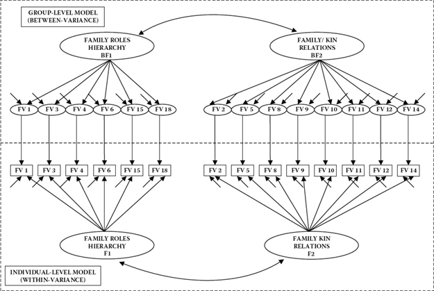
Figure 12.1. Hypothesized multilevel model of factorial structure for the Family Values Scale (Georgas, 1999).
Current Approach to Analyses of the Hypothesized MLV Model
Prior to walking you through stages of analyses related to this application, I wish first to summarize characteristics of the data as this may be instructive in helping you understand why I chose the analytic approach taken here; these are as follows.
Sample Size
Because 5,482 university students from 27 countries responded to 14 items on the FV Scale, sample size for the individual (or lower) level of the hierarchical structure is 5,482 and that of the group (or higher) level is 27. As data preparation in the original study of the FV Scale across cultures (Georgas, Berry, van de Vijver, Kagitcibasi, & Poortinga, 2006) involved replacement of the relatively few missing values with regression-based estimates to which an error component was added, all FV Scale item scores are complete.
Item Scaling
Although items on the FV Scale are admittedly categorical, the number of scale points is seven. Given evidence that, as the number of scale points increases, ordinal data behave more closely to interval data (Boomsma, 1987; Rigdon, 1998), outcome variables in the present analyses are treated as if they are continuous.
Estimation
Given that the MLR estimator is now default in Mplus for MLV modeling and is becoming the preferred approach to these analyses, this estimator is used first in MLV analyses of the FV Scale. However, if presented with analytic difficulties, possibly due to the small sample size at the higher level, analyses are subsequently based on the MUML estimator.
The Analytic Process
Analyses of the data are conducted in three different stages. First, based on the full sample covariance matrix that ignores the grouping aspect of the data, we conduct a CFA as a means of testing the validity of the hypothesized two-factor structure shown in Figure 12.1. In the event that this analysis suggests model modifications that are rational and substantively defensible, the model is modified accordingly.
Second, provided with evidence of adequate fit of the single-level CFA model, the factor structure pertinent to both the individual and group levels of the data is tested in a simultaneous analysis of the MLV model based on MLR estimation.
Third, given that intraclass correlation coefficients (ICCs) of the observed variables (the items) are automatically reported in the simultaneous analysis conducted at Step 2, these values are examined as a means of justification (or nonjustification) of continued analyses of the MLV model. ICC values range from 0.0 to 1.0 and represent the proportion of between-group variance compared with total variance. Given findings of ICCs close to zero, it is meaningless to model within and between levels of the structure, and, thus, a conventional SEM approach to the analyses will yield reasonable and unbiased estimates (Julian, 2001). Muthén (1997) noted that, typically, ICC values tend to range from 0.00 to 0.50 and suggested that when group sizes exceed 15 and findings yield ICC values of 0.10 or larger, the multilevel structure of the data should definitely be modeled. More recently, however, Julian (2001) and Selig et al. (2008) have recommended that even with findings of ICC values less than 0.10, the hierarchical structure should not be ignored.
Finally, as noted earlier, in the event that MLV modeling of the data rendered reasonable results, two suggestions are provided regarding subsequent analyses that might be considered in an attempt to gather further evidence of construct validity related to the FV Scale.
Mplus Input File Specification and Output File Results
CFA of FV Scale Structure
Input File
As noted earlier, initial analysis of the data involved testing for the validity of the hypothesized structure of the FV Scale based on the total covariance matrix with no concern regarding hierarchical structure. The input file for this initial analysis is shown in Figure 12.2. Given that you are now very familiar with CFA Mplus model specification, I draw your attention to only two aspects of this file. First, note that the variable COUNTRY is not included in the USEVARIABLES command as it is not, of course, part of the factor analytic structure of the FV Scale. Second, given that the data are nonnormally distributed, the MLM estimator is used.
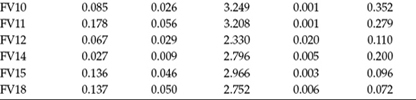
A review of the output file for this analysis reveals a fairly well-fitting model as follows: χ2(76) = 1470.341, Comparative Fit Index (CFI) = 0.938, Root Mean Square Error of Approximation (RMSEA) = 0.058, and Standardized Root Mean Square Residual (SRMR) = 0.051. Not surprisingly, given the total sample size, all parameters were found to be statistically significant. Although these results are supportive of the hypothesized factor structure, a review of the modification indices (MIs) indicated the need for possible respecification of the model. These MI values are presented in Table 12.1.
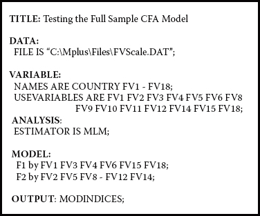
Figure 12.2. Mplus input file for test of confirmatory factor analysis (CFA) model for full sample.
In examining these MIs, you will note five very large values that appear in bolded text—three representing possible cross-loadings (F1 by FV9; F1 by FV14; F2 by FV1) and two possible residual covariances (FV12 with FV9; FV15 with FV11). Because particular items will be of interest at various stages of these MLV analyses, abbreviated content of all 14 FV items used in this application (see earlier explanation of this number) is presented in Table 12.2. Thus, essence of the items pertinent to these large MI values can be observed in this table.
As I have stressed throughout this book, however, any modifications to a postulated model should be made only on the basis of substantive meaningfulness. Adhering to this edict, I consider modifications based on only the first two MIs in Table 12.1 to fall into this category as each would appear to represent an aspect of familial hierarchical structure. Accordingly, these two cross-loadings represent the regression of FV9 and FV14 on Factor 1 (Family Roles Hierarchy).
Provided with substantive justification for modification of the hypothesized CFA structure, the model was subsequently respecified to include these two additional parameters, albeit pertinent to the individual level only. Goodness-of-fit indices related to this respecified model were χ2(74) = 1101.256, CFI = 0.954, RMSEA = 0.050, and SRMR = 0.038. Both cross-loadings were found to be statistically significant. A schematic representation of this modified model is shown in Figure 2.3.
Table 12.1 Mplus Output: Selected Modification Indices (MIs)
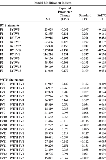
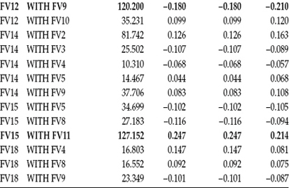
Table 12.2 Abbreviated FV Scale Item Content
| Item | Abbreviated Content |
| 1 | Father should be head of family. |
| 2 | Should maintain good relationships with relatives. |
| 3 | Mother's place is at home. |
| 4 | In family disputes, mother should be go-between. |
| 5 | Parents should teach proper behavior. |
| 6 | Father should handle the money. |
| 8 | Children should take care of old parents. |
| 9 | Children should help with chores. |
| 10 | Problems should be resolved within the family. |
| 11 | Children should obey parents. |
| 12 | Children should honor family's reputation. |
| 14 | Children should respect grandparents. |
| 15 | Mother should accept father's decisions. |
| 18 | Father should be breadwinner |
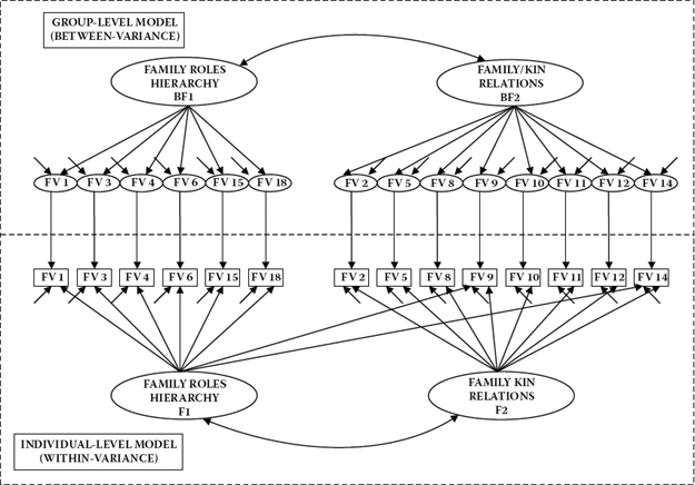
Figure 12.3. Multilevel model respecified at the individual level.
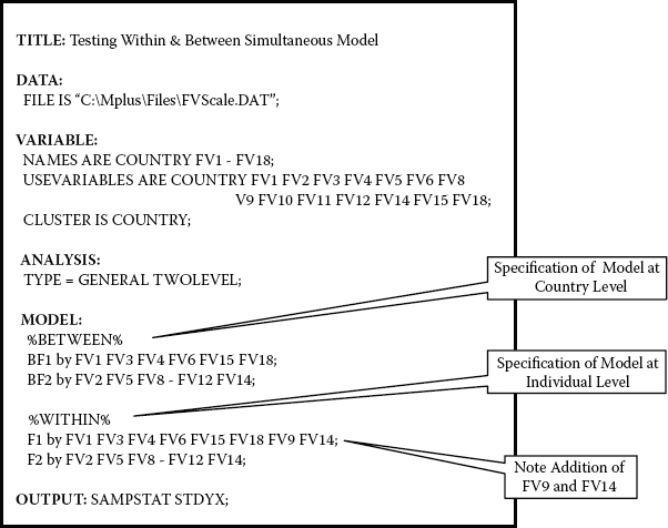
Figure 12.4. Mplus input file for test of modified multilevel model based on MLR estimation.
MLV Model of FV Scale Structure
Input File
Having established a better fitting model in representing the FV Scale factor structure, we are now ready to conduct a simultaneous analysis of this structure relative to both the individual and country levels of the data. The input file pertinent to this analysis is presented in Figure 12.4.
In reviewing this file, there are several points to note. First, in contrast to the input file for full-sample tests of the CFA model (see Figure 12.2), the variable of Country has been added to the USEVARIABLES subcommand. Second, there is now a CLUSTER subcommand appearing under the VARIABLE command that is used to identify the grouping variable. Third, the ANALYSIS command identifies the TYPE of analysis to be GENERAL as applied to a two-level model. It should be noted, however, that if a breakdown of sample size per group is of interest, this information can be obtained simply by replacing the term GENERAL with BASIC. No estimator is noted here as analyses are based on robust maxium likelihood (MLR) estimation, which is default. Fourth, under the MODEL command, as indicated in Figure 12.4, the %BETWEEN% and %WITHIN%. subcommands provide for specification of the country (higher) and individual (lower) levels of the MLV model, respectively. Finally, note the additional specification of FV9 and FV14 as factor loadings on Factor 1 at the individual level, but not at the country level.
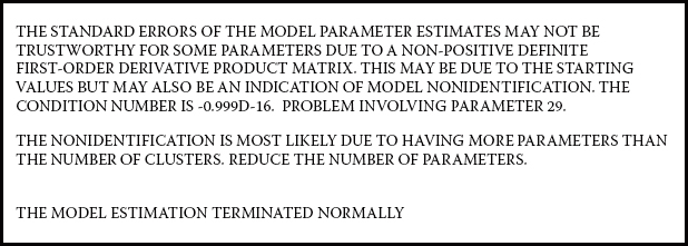
Figure 12.5. Mplus output file: Error message associated with (MLR) estimated model.
Unfortunately, although the model terminated normally, an error message related to the higher level of the model appeared in the output. This message is presented in Figure 12.5.
As you can see from the error message text, the problem involves a condition of nonidentification at the higher level likely due to the small number of countries included in the higher level sample. Indeed, a review of model specifications reveals the number of estimated parameters (43) to exceed the number of groups (27); the estimated parameters comprise 14 item intercepts, 12 factor loadings, 14 residuals, 2 factor variances, and 1 factor covariance. To obtain an overidentified model, I would therefore need to delete at least 17 parameters from the estimation process. Considering only the item intercepts and three residual variances to be the most logical and reasonable parameters eligible for deletion, I subsequently modified the input file to exclude estimation of the 14 item intercepts as well as the three residual variances having the lowest estimated values from this first analysis (FV5, FV14, and FV9, respectively) at the country level. This modified input file is shown in Figure 12.6.
Unfortunately, despite this reduction of estimated parameters at the higher level of the model, the same error message appeared in the output, although the analysis again terminated normally. An interesting comparison between these two models, however, was the substantial decrement in model fit. Whereas goodness-of-fit statistics for Model 1 were χ2(150) = 796.780, CFI = 0.993, RMSEA = 0.028, and SRMR (between) = 0.117, results were χ2(167) = 1312.682, CFI = 0.881, RMSEA = 0.035, and SRMR (between) = 0.335 for Model 2 (intercept and three residual variances fixed to 0.0). Thus, although it seems evident that specifications pertinent to Model 1 are the more appropriate of the two, the smallness of the cluster size (of countries) is problematic when analyses are based on the MLR estimator.
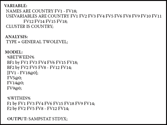
Figure 12.6. Mplus input file for test of multilevel model with reduction in number of estimated parameters.
Presented with these results, and in the sole interest of providing you with a window into the basics of MLV modeling, I consider it worthwhile to continue these MLV analyses based on the MUML rather than on the MLR estimator, albeit with the critically important caveat that whereas the MUML estimator assumes multivariate normality, our data here are nonnormally distributed. Thus, with the exception of the additional subcommand ESTIMATOR IS MUML, the input file shown in Figure 12.4 remains the same.
Importantly, analyses based on the MUML estimator terminated normally with no presentation of error messages. This information is particularly notable given results from two studies of MUML robustness (Hox & Maas, 2001; Yuan & Hayashi, 2005) in which results indicated the likelihood of increased occurrences of inadmissible solutions, particularly if the number of groups at the higher level was less than 50. On the other hand, presented with an admissible solution, Hox and Maas (2001) posited that the factor loadings are generally accurate, although the possibility remains that the residual variances may be underestimated and the standard errors small.
Table 12.3 Mplus Output: Estimated Intraclass Correlation Coefficients
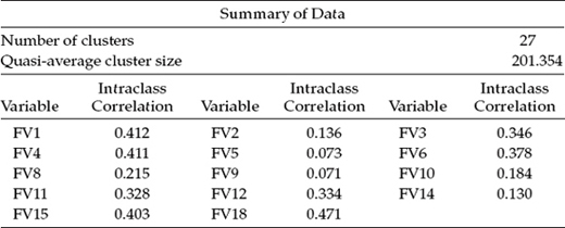
Intraclass Correlations
Initial information in the output file presents a “Summary of the Data” that includes the number of clusters in the analysis, the quasi-average cluster size, and the ICCs pertinent to each of the observed variables (the items). These results are reported in Table 12.3.
Of substantial interest here are the ICC values, which ranged from .071 to .471, with 12 of the 14 values being greater than 0.10 (see Muthén, 1997). In light of these ICC values, it is clear that the effects of culture are strongly impacting the FV Scale scores. Indeed, a review of the content related to FV Scale items yielding the six highest ICC values (FV18, FV1, FV4, FV15, FV6, and FV3; see Table 12.2) reveals all to bear on the perceived roles of mothers and fathers in the family, which I believe presents a pretty clear picture of why responses to the items should vary so widely across the 27 countries.
Model Fit
Tests of model fit for this MLV model, as reported in Table 12.4, reveal a fairly well-fitting two-level model in accordance with both the CFI and RMSEA goodness-of-fit values. Note, however, that two SRMR values are reported—one for the within (or individual) level (0.036) and one for the between (or country) level (0.112). As such, these results suggest that the model fits the data better at the individual than at the country level.
An interesting conundrum with respect to MLV modeling, however, is that these goodness-of-fit indices relate to the entire model. As such, they reflect the extent to which the model fits the data within the framework of the within-group model as well as the between-group model, a practice that Ryu and West (2009) equated with single-level SEM analyses. Given that, typically, sample size for the within-group is larger than that of the between-group, the former portion of the model tends to dictate these model fit values (Hox, 2002). Ideally, then, it would seem preferable that model fit be evaluated separately for each of the two levels. Unfortunately, preparation of these two matrices for separate model fit assessment is not a simple and straightforward process and, thus, is not included here. However, for readers who may be interested in performing these analyses, Hox (2002) suggested two possible approaches that can be taken. More recently, Ryu and West (2009), based on simulated data and ML estimation (thus assuming multivariate normality and balanced grouping), investigated two level-specific approaches to determining model fit in MLV models: one based on their proposed partially saturated model method, and the other on a segregating method proposed by Yuan and Bentler (2007). In both cases, these level-specific methods were successful in targeting evidence of misfit at the group level. Given the widely known limitations associated with the standard approach to assessment of fit in MLV modeling, it seems likely that researchers will increasingly seek out methods that allow them to detect misspecification specific to each level separately.
Table 12.4 Mplus Output: Selected Goodness-of-Fit Statistics
| Tests of Model Fit | ||
| Chi-Square Test of Model Fit | ||
| Value | 1245.684 | |
| Degrees of freedom | 150 | |
| p-value | 0.0000 | |
| CFI/TLI | ||
| CFI | 0.940 | |
| TLI | 0.928 | |
| Root Mean Square Error of Approximation (RMSEA) | ||
| Estimate | 0.037 | |
| 90 percent confidence interval (CI) | 0.035 | 0.038 |
| Probability RMSEA <= .05 | 1.000 | |
| Standardized Root Mean Square Residual (SRMR) | ||
| Value for within | 0.036 | |
| Value for between | 0.112 | |
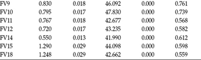
Parameter Estimates
Both the unstandardized and standardized estimates are presented in Table 12.5 for the individual (within-group) model and in Table 12.6 for the country (between-group) model. In reviewing the unstandardized estimates in these output files, you will quickly observe that all parameters estimates are statistically significant at both levels of the MLV model.
Table 12.5 Mplus Output: Selected Unstandardized and Standardized Estimates for Individual Level
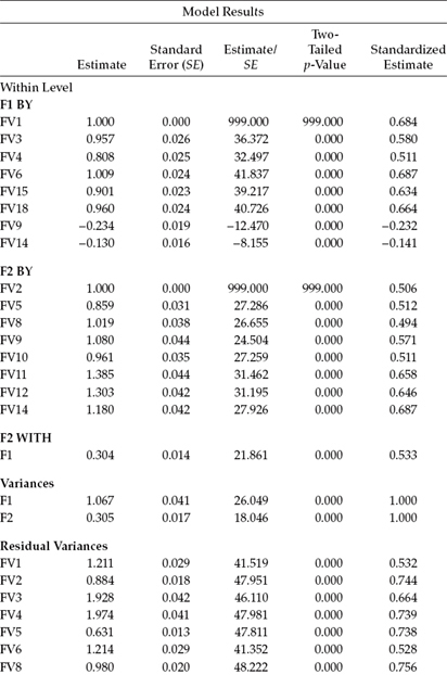
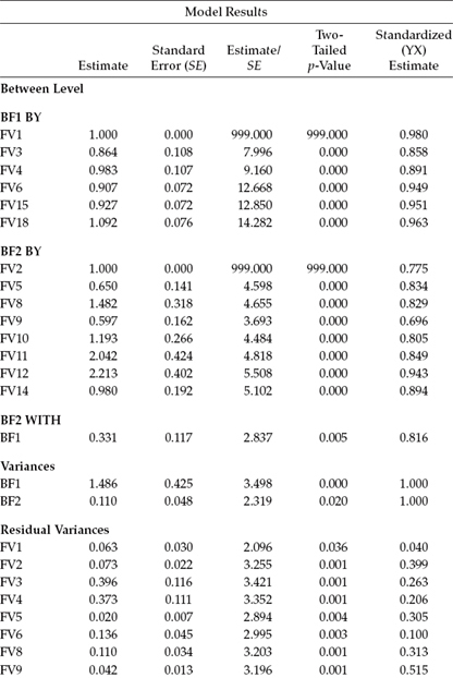
An overview of the standardized estimates reveals the factor loadings for all 14 items of the FV Scale to be larger for the country level than for the individual level. Indeed, presented with sufficient ICC values and, thus, stable loadings, it is typical for factor loadings to be larger at the between-group level than at the individual level. The reason for this common finding derives from the fact that analyses at the between-group level are based on the means, which, of course, are more reliable than raw scores, and thus much of the measurement error has been eliminated.
An important aspect of MLV modeling is that the factor loadings are standardized separately at the individual and group levels. As such, there is no relation in the proportion of variance accounted for in one level versus the other level. In a comparison of standardized loadings reported in Tables 12.5 and 12.6, for example, we can observe that whereas the loading of Item 3 (FV3) accounted for 33.6% (0.5802) of the variability in F1 at the individual level, it accounted for 73.6% (0.8582) at the country level. Likewise, there is no correspondence between interpretations of F1 at the individual versus the country levels.
The final piece of information provided in the output file relates to the multiple correlation (R2) values at each level. In general terms, these values convey the strength of each item in measuring its target factor. Consistent with the standardized estimates reported in Tables 12.5 and 12.6, these R2 values are substantially higher at the country level than at the individual level. Of interest here, however, is that whereas at the country level, the strongest factor loading was associated with the first item of the FV Scale (FV1; 0.960), at the individual level it was associated with Item 6 (FV6; 0.472), with both items designed to measure Factor 1. These multiple correlations are presented in Table 12.7.
Table 12.6 Mplus Output: Selected Unstandardized and Standardized Estimates for Country Level
Potential Analytic Extensions
In my introduction of the model to be illustrated in this application, I noted that only the initial stages of testing for evidence of construct validity bearing on the FV Scale when used with hierarchically structured data would be included here. However, at that time, I stated that I would offer two suggestions on how this work might be meaningfully extended. I now address these potential extensions.
One very logical set of analyses that could contribute importantly to this construct validity work is that of testing for model invariance across individual and country levels. Indeed, given the relatively good fit of the MLV model to the data representing both structural levels, these proposed analyses would appear to be strongly justified. Recall again, however, that whereas the MUML estimator assumes multivariate normality, the data used here are nonnormally distributed. Thus, caution needs to be taken into account in any interpretation of results. Accordingly, analyses would focus on testing the equivalence of factorial structure for the FV Scale across levels. To assist you in initiating these analyses, the related Mplus input file is shown in Figure 12.7.
This input file represents the initial test for equivalence of the commonly specified factor loadings across individual and country levels. I wish to draw your attention to several important features regarding these specifications. First, consistent with the specification of equality constraints involving single parameters across groups (see, e.g., Chapters 7, 8, and 9), these constraints operate in the same way within the context of MLV modeling. That is, each equality constraint is accompanied by a parenthesized number that is identically assigned at the individual (within) and country (between) levels. Second, constraints have been specified for only the original target factor loadings. Thus, although the cross-loadings of FV9 and FV14 are specified as freely estimated parameters for the WITHIN model, they are not listed with parenthesized assigned numbers. Third, note that specification of the factor loadings is included only at the individual level (see the WITHIN model).6 Finally, because the entire factor-loading pattern is not specified for the country-level model (see the BETWEEN model), it is necessary to identify the loading intended as the referent variable for purposes of model identification and latent variable scaling. Given that the first variable of each factor congeneric group (FV1, FV2) will be automatically fixed to 1.0 for the individual level, these same factor-loading parameters must be specified at the country level; consistent with the individual level, they will also be constrained to 1.0 by default.
Table 12.7 Mplus Output: Multiple Correlations for Individual and Country Levels
| R-Square | ||
| Within Level | ||
| Observed Variable | Estimate | |
| FV1 | 0.468 | |
| FV2 | 0.256 | |
| FV3 | 0.336 | |
| FV4 | 0.261 | |
| FV5 | 0.262 | |
| FV6 | 0.472 | |
| FV8 | 0.244 | |
| FV9 | 0.239 | |
| FV10 | 0.261 | |
| FV11 | 0.432 | |
| FV12 | 0.418 | |
| FV14 | 0.388 | |
| FV15 | 0.402 | |
| FV18 | 0.441 | |
| Between Level | ||
| Observed Variable | Estimate | |
| FV1 | 0.960 | |
| FV2 | 0.601 | |
| FV3 | 0.737 | |
| FV4 | 0.794 | |
| FV5 | 0.695 | |
| FV6 | 0.900 | |
| FV8 | 0.687 | |
| FV9 | 0.485 | |
| FV10 | 0.648 | |
| FV11 | 0.721 | |
| FV12 | 0.890 | |
| FV14 | 0.800 | |
| FV15 | 0.904 | |
| FV18 | 0.928 | |
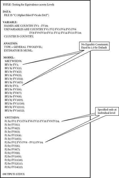
Figure 12.7. Mplus input file for test of factor-loading measurement equivalence across level.
Consistent with results in testing the unconstrained MLV model, those for the equivalence MLV model revealed a relatively good fit to the hierarchically structured data and minimal difference between the ad hoc fit indices (χ2[62] = 1300.563; CFI = 0.938; RMSEA = 0.036; SRMR [within] = 0.036; SRMR [between] = 0.214). Whereas the SRMR remained virtually the same at the individual level, it showed a decrement in fit at the country level (0.214 versus 0.112).
Of interest now, of course, is the extent to which this constrained MLV model differs from the unconstrained MLV model. Given that the constrained model is nested within the unconstrained model, we could take the difference between the MUML χ2 values had these analyses been based on data that were normally distributed and minimally unbalanced (K. Yuan, personal communication, December 2010). Alternatively, had we been successful in our use of MLR estimation, we could have computed the corrected ΔMLR χ2 value. However, given that neither of these options is relevant here, it is inappropriate to make any interpretations on a ΔMUML χ2 value.
A second potential avenue of extended MLV analyses for these data is to consider the inclusion of possibly influential covariates. For example, given the substantial size of the ICCs evidenced in these analyses, we could consider what type of cultural phenomena might possibly contribute to the variability of FV Scale scores across these widely diverse 27 cultures. Indeed, two that come immediately to mind are those of affluence and religion. As such, these two covariates could be added to the model, and their impact on the two factors of Family Roles Hierarchy and Family/Kin Relations determined.
Notes
| 1. | There are essentially two classes of MLV procedures: (a) latent variable MLV conducted within the framework of SEM, and (b) multiple regression MLV representing a multilevel version of the usual multiple regression model. As this chapter focuses only on SEM MLV modeling, readers interested in applications based on a multiple regression paradigm are referred to Bickel (2007), Heck and Thomas (2009), and Hox (2002, 2010). |
| 2. | Original data derived from a large project designed to measure family functioning across 30 cultures (Georgas et al., 2006). I am indebted to James Georgas for his generosity in permitting me to use a portion of these data as a means to illustrate the application of MLV modeling in this chapter. |
| 3. | Aggregated data derived through the summation of individual-level data have been termed an ecological analysis. |
| 4. | As noted by Kaplan et al. (2009), development of the EM algorithm for estimation (Dempster, Laird, & Rubin, 1977) was based on the premise of incomplete data. |
| 5. | In an effort to maximize ecocultural variation in known family-related context variables such as economic factors and religion, countries were selected from north, central, and south America; north, east, and south Europe; north, central, and south Africa; the Middle East; west and east Asia; and Oceania. |
| 6. | I don't want to leave the impression that it is incorrect to include specification of all factor loadings for the BETWEEN model as this is not so. However, if the full specification is included for the BETWEEN model, all factor-loading estimates, except for the referent variable loading, appear twice in the output file. For example, the loadings reported for F1 are FV1, FV3, FV4, FV6, FV15, FV18, FV3, FV4, FV6, FV15, and FV18. |