chapter 7

Testing the Factorial Equivalence
of a Measuring Instrument

Analysis of Covariance Structures

Up to this point, all applications have illustrated analyses based on single samples. In this section, however, we focus on applications involving more than one sample where the central concern is whether or not components of the measurement model and/or the structural model are invariant (i.e., equivalent) across particular groups of interest. Throughout this chapter and others involving multigroup applications, the terms invariance and equivalence are used synonymously (and, likewise, the adjectives invariant and equivalent); use of either term is merely a matter of preference.

In seeking evidence of multigroup invariance, researchers are typically interested in finding the answer to one of five questions. First, do the items comprising a particular measuring instrument operate equivalently across different populations (e.g., gender, age, ability, culture)? In other words, is the measurement model group-invariant? Second, is the factorial structure of a single instrument or of a theoretical construct equivalent across populations as measured either by items of a single assessment measure or by subscale scores from multiple instruments? Typically, this approach exemplifies a construct validity focus. In such instances, equivalence of both the measurement and structural models is of interest. Third, are certain paths in a specified causal structure equivalent across populations? Fourth, are the latent means of particular constructs in a model different across populations? Finally, does the factorial structure of a measuring instrument replicate across independent samples drawn from the same population? This latter question, of course, addresses the issue of cross-validation. Applications presented in this chapter, as well as the next two chapters, provide you with specific examples of how each of these questions can be answered using structural equation modeling (SEM) based on the Mplus program. The applications illustrated in Chapters 7 and 9 are based on the analysis of covariance structures (COVS), whereas the application in Chapter 8 is based on the analysis of mean and covariance structures (MACS). When analyses are based on COVS, only the sample variances and covariances are of interest; all single-group applications illustrated thus far in the book have been based on the analysis of COVS. In contrast, when analyses are based on MACS, the modeled data include the sample means, as well as the sample variances and covariances. Details related to the MACS approach to invariance are addressed in Chapter 8.

In this first multigroup application, we test hypotheses related to the invariance of a single measuring instrument across two different panels of teachers. Specifically, we test for equivalency of the factorial measurement (i.e., scale items) of the Maslach Burnout Inventory (MBI; Maslach & Jackson, 1986)¹ and its underlying latent structure (i.e., relations among dimensions of burnout) across elementary and secondary teachers. Purposes of the original study, from which this example is taken (Byrne, 1993), were (a) to test for the factorial validity of the MBI separately for each of three teacher groups; (b) given findings of inadequate fit, to propose and test an alternative factorial structure; (c) to cross-validate this structure over independent samples within each teacher group; and (d) to test for the equivalence of item measurements and theoretical structure across the three teaching panels. Only analyses bearing on tests for invariance across calibration samples of elementary (n = 580) and secondary (n = 692) teachers are of interest in the present chapter.² Before reviewing the model under scrutiny, however, I wish first to provide you with a brief overview of the general procedure involved in testing for invariance across groups.

Testing Multigroup Invariance: The General Notion

Development of a procedure capable of testing for multigroup invariance derives from the seminal work of Jöreskog (1971b). Accordingly, Jöreskog recommended that all tests for equivalence begin with a global test of the equality of covariance structures across the groups of interest. Expressed more formally, this initial step tests the null hypothesis (H₀), Σ₁ = Σ₂ = … Σ_G where Σ is the population variance–covariance matrix, and G is the number of groups. Rejection of the null hypothesis then argues for the nonequivalence of the groups and, thus, for the subsequent testing of increasingly restrictive hypotheses in order to identify the source of nonequivalence. On the other hand, if H₀ cannot be rejected, the groups are considered to have equivalent covariance structures, and, thus, tests for invariance are not needed. Presented with such findings, Jöreskog recommended that group data should be pooled and all subsequent investigative work based on single-group analyses.

Although this omnibus test appears to be reasonable and fairly straightforward, it often leads to contradictory findings with respect to equivalencies across groups. For example, sometimes the null hypothesis is found to be tenable, yet subsequent tests of hypotheses related to the equivalence of particular measurement or structural parameters must be rejected (see, e.g., Jöreskog, 1971b). Alternatively, the global null hypothesis may be rejected, yet tests for the equivalence of measurement and structural invariance hold (see, e.g., Byrne, 1988a). Such inconsistencies in the global test for equivalence stem from the fact that there is no baseline model for the test of invariant variance–covariance matrices, thereby making it substantially more restrictive than is the case for tests of invariance related to sets of model parameters. Indeed, any number of inequalities may possibly exist across the groups under study. Realistically, then, testing for the equality of specific sets of model parameters would appear to be the more informative and interesting approach to multigroup invariance. Thus, tests for invariance typically begin with a model termed the configural model (to be discussed shortly).

In testing for invariance across groups, sets of parameters are put to the test in a logically ordered and increasingly restrictive fashion. Depending on the model and hypotheses to be tested, the following sets of parameters are most commonly of interest in answering questions related to multigroup invariance: (a) factor loadings, (b) factor covariances, (c) structural regression paths, and (d) latent factor means. Historically, the Jöreskog tradition of invariance testing held that the equality of residual variances and their covariances should also be tested. However, it is now widely accepted that this test for equivalence not only is of least interest and importance (Bentler, 2005; Widaman & Reise, 1997) but also may be considered somewhat unreasonable (Little, Card, Slegers, & Ledford, 2007) and indeed not recommended (see Selig, Card, & Little, 2008). Two important exceptions to this widespread consensus, however, are in testing for multigroup equivalence related to item reliability (see, e.g., Byrne, 1988a) as well as for commonly specified residual (i.e., error) covariances.

The Testing Strategy

Testing for factorial equivalence encompasses a series of steps that build upon one another and begins with the determination of a separate baseline model for each group. This model represents one that best fits the data from the perspectives of both parsimony and substantive meaning fulness. Addressing this somewhat tricky combination of model fit and model parsimony, it ideally represents one for which fit to the data and minimal parameter specification are optimal. Following completion of this preliminary task, tests for the equivalence of parameters are conducted across groups at each of several increasingly stringent levels.

Once the group-specific baseline models have been established, testing for invariance entails a hierarchical set of steps that typically begins with the determination of a well-fitting multigroup baseline model for which sets of parameters are put to the test of equality in a logically ordered and increasingly restrictive fashion. In technical terms, this model is commonly termed the configural model and is the first and least restrictive one to be tested (Horn & McArdle, 1992). With this initial multigroup model, only the extent to which the same pattern (or configuration) of fixed and freely estimated parameters holds across groups is of interest, and thus no equality constraints are imposed. In contrast to the configural model, all remaining tests for equivalence involve the specification of cross-group equality constraints for particular parameters. In general terms, the first set of steps in testing for invariance focuses on the measurement model (Jöreskog, 1971b). As such, all parameters associated with the observed variables and their linkage to the latent factors in a model are targeted; these include the factor loadings, observed variable intercepts, and residual variances. Because each of these three tests for invariance represents an increased level of restrictiveness, Meredith (1993) categorized them as weak, strong, and strict tests of equivalence, respectively.

Once it is known which measures are group-invariant, these parameters are constrained equal while subsequent tests of the structural parameters (factor variances/covariances, regression paths, and latent means) are conducted. As each new set of parameters is tested, those known to be group invariant are cumulatively constrained equal across groups. Thus, the process of determining the group-invariant measurement and structural parameters involves the testing of a series of increasingly restrictive hypotheses.

It is important to note that, although I have listed all parameters that can be considered eligible for tests of invariance, the inclusion of all in the process is not always necessary or reasonable. For example, although some researchers contend that tests for invariant observed variable intercepts should always be conducted (e.g., Little, 1997; Little et al., 2007; Meredith, 1993; Selig et al., 2008), others argue that tests related only to the factor loadings, variances, and covariances may be the most appropriate approach to take in addressing the issues and interests of a particular study (see, e.g., Cooke, Kosson, & Michie, 2001; Marsh, 1994, 2007; Marsh, Hau, Artelt, Baumert, & Peschar, 2006). Construct validity studies pertinent to a particular assessment scale, such as the one under study in the current application (Byrne, 1993), or to a theoretical construct (e.g., Byrne & Shavelson, 1986) exemplify such research. For additional articles addressing practical issues related to tests for invariance, readers are referred to Byrne (2008) and Byrne and van de Vijver (2010). We turn now to the invariance tests of interest in the present chapter.

As noted earlier, this multigroup application is based solely on the analysis of COVS. I consider this approach to the topic less complex (compared with that of MACS) and more appropriate at this time for at least three important reasons. First, this application represents your first overview of, and experience with, multigroup analyses; thus, I prefer to keep things as simple as possible. Second, the current application represents a construct validity study related to a measuring instrument, the major focus being the extent to which its factorial structure is invariant across groups; of primary interest are the factor loadings, variances, and covariances. Finally, group differences in the latent means are of no particular interest in the construct validity study, and, thus, tests for invariant intercepts are not relevant in this application.

Testing Multigroup Invariance Across Independent Samples

Our focus here is to test for equivalence of the MBI across elementary and secondary teachers. Given that details regarding the structure of this measuring instrument, together with a schematic portrayal of its hypothesized model structure, were presented in Chapter 4, this material is not repeated here. As noted earlier, a necessary requisite in testing for multigroup invariance is the establishment of a well-fitting baseline model structure for each group. Once these models are established, they (if two different baseline models are ascertained) represent the hypothesized multigroup model under test. We turn now to these initial analyses of MBI structure as they relate to elementary and secondary teachers.

The Hypothesized Model

As noted previously, the model under test in this initial multigroup application is the same postulated three–factor structure of the MBI that was tested in Chapter 4 for male elementary teachers. Thus, the same model of hypothesized structure shown in Figure 4.1 holds here. As such, it serves as the initial model tested in the establishment of baseline models for the two groups of teachers.

Establishing Baseline Models: The General Notion

Because the estimation of baseline models involves no between-group constraints, the data can be analyzed separately for each group. However, in testing for invariance, equality constraints are imposed on particular parameters, and, thus, the data for all groups must be analyzed simultaneously to obtain efficient estimates (Bentler, 2005; Jöreskog & Sörbom, 1996); the pattern of fixed and free parameters nonetheless remains consistent with the baseline model specification for each group. However, it is important to note that measuring instruments are often group specific in the way they operate, and, thus, it is possible that baseline models may not be completely identical across groups (see Bentler, 2005; Byrne, Shavelson, & Muthén, 1989). For example, it may be that the best-fitting model for one group includes a residual covariance (see, e.g., Bentler, 2005) or a cross-loading (see, e.g., Byrne, 1988b, 2004; Reise, Widaman, & Pugh, 1993), whereas these parameters may not be specified for the other group. Presented with such findings, Byrne et al. (1989) showed that by implementing a condition of partial measurement invariance, multigroup analyses can still continue. As such, some but not all measurement parameters are constrained equal across groups in the testing for structural equivalence (or latent factor mean differences, if applicable). It is important to note, however, that over the intervening years, the concept of partial measurement equivalence has sparked a modest debate in the technical literature (see Millsap & Kwok, 2004; Widaman & Reise, 1997). Nonetheless, its application remains a popular strategy in testing for multigroup equivalence and is especially so in the area of cross-cultural research. The perspective taken in this book is consistent with that of Muthén and Muthén (2007–2010) in the specification of partial measurement invariance where appropriate in the application of invariance-testing procedures.

Establishing Baseline Models: Elementary and Secondary Teachers

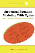
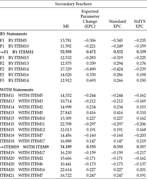
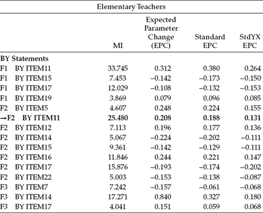
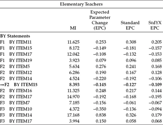
In testing for the validity of the three-factor structure of the MBI (see Figure 4.1), findings were consistent in revealing goodness-of-fit statistics for this initial model that were less than optimal for both elementary (MLM χ²_[206] = 826.573; CFI = 0.857; RMSEA = 0.072 ; SRMR = 0.068) and secondary (MLM χ²_[206] = 999.359; CFI = 0.836; RMSEA = 0.075; SRMR = 0.077) levels. Consistent with findings for male elementary teachers (see Chapter 4), three exceptionally large residual covariances and one cross loading contributed to the misfit of the model for both teacher panels. The residual covariances involved Items 1 and 2, Items 6 and 16, and Items 10 and 11; the cross-loading involved the loading of Item 12 on Factor 1 (Emotional Exhaustion) in addition to its targeted Factor 3 (Personal Accomplishment). (For discussion related to possible reasons for these misfitting parameters, readers are referred to Chapter 4.)³ To observe the extent to which these four parameters eroded fit of the originally hypothesized model to data for elementary and secondary teachers, we turn to Table 7.1, where the Modification Index (MI) results pertinent to the BY and WITH statements are shown. In reviewing both the MIs and expected parameter change (EPC) statistics for elementary teachers, it is clear that all four parameters are contributing substantially to model misfit, with the residual covariance between Item 6 and Item 16 exhibiting the most profound effect.

Table 7.1 Mplus Output for Initially Hypothesized Model: Selected Modification Indices (MIs)

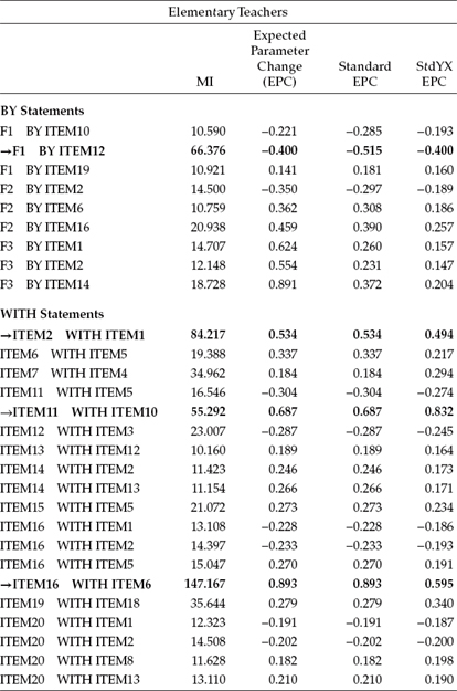
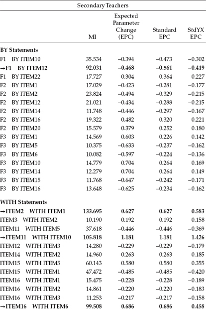
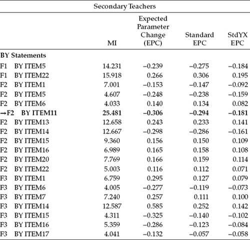
Turning to these results, as they relate to secondary teachers, we see precisely the same pattern, albeit the effect would appear to be even more pronounced than it was for elementary teachers. However, note one slight difference between the two groups of teachers regarding the impact of these four parameters on model misfit. Whereas the residual covariance between Items 6 and 16 was found to be the most seriously misfitting parameter for elementary teachers, the residual covariance between Items 1 and 2 held this dubious honor for secondary teachers.

As noted in Chapter 4, presented with MI results indicative of several possibly misspecified parameters, it is strongly recommended that only one new parameter at a time be included in any respecification of the model. In the present case, however, given our present knowledge of these four misfitting parameters in terms of both their performance and justified specification for male elementary teachers (see Chapter 4), I consider it appropriate to include all four in a post hoc model, labeled as Model 2. Estimation of this respecified model, for each teacher group, yielded model fit statistics that were significantly improved from those for the initially hypothesized model (elementary: ΔMLM χ²_[4] = 1012.654, p < .001; secondary: ΔMLM χ²_[4] = 1283.053, p < .001);⁴ all newly specified parameters were statistically significant. Model goodness-of-fit statistics for each teacher group were as follows:

Elementary teachers: MLM χ²₍₂₀₂₎ = 477.666; CFI = 0.936;
RMSEA = 0.049; SRMR = 0.050

Secondary teachers: MLM χ²₍₂₀₂₎ = 587.538; CFI = 0.920;
RMSEA = 0.053; SRMR = 0.05

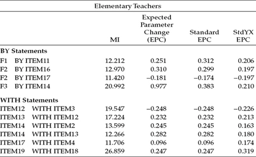
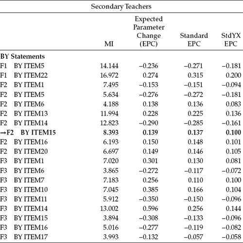
Let's turn now to Table 7.2, where the MI results pertinent to Model 2 are presented. In reviewing this information for elementary teachers, we observe two MIs under the WITH statements that are substantially larger than all other MIs (ITEM7 with ITEM4; ITEM19 with ITEM18); both represent residual covariances. Of the two, only the residual covariance between Items 7 and 4 is substantively viable in that there is a clear overlapping of item content. In contrast, the content of Items 19 and 18 exhibits no such redundancy, and, thus, there is no reasonable justification for including this parameter in a succeeding Model 3.

Table 7.2 Mplus Output for Model 2: Selected Modification Indices (MIs)

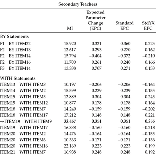
In reviewing the results for secondary teachers, on the other hand, it appears that more work is needed in establishing an appropriate baseline model. I make this statement based on two considerations: (a) The model does not yet reflect a satisfactorily good fit to the data (CFI = 0.920); and (b) in reviewing the MIs in Table 7.2, we observe one very large misspecified parameter representing the loading of Item 11 on Factor 1 (F1 by ITEM11), as well as another substantially large MI representing a residual covariance between Items 19 and 9, both of which can be substantiated as substantively meaningful parameters. Following my previous caveat, we proceed in specifying only one of these parameters at this time. Given the substantially large MI representing the cross-loading of Item 11 on Factor 1, only this parameter is included in our next post hoc model (Model 3 for secondary teachers). MI results derived from this analysis of Model 3 will then determine if further respecification is needed. Findings are reported in Table 7.3.

Results from the estimation of Model 3 for elementary teachers yielded goodness-of-fit statistics that represented a satisfactorily good fit to the data (MLM χ²_[201] = 451.060; CFI = 0.942; RMSEA = 0.046; SRMR = 0.049) and a corrected difference from the previous model (Model 2) that was statistically significant (ΔMLM χ²_[1] = 9.664, p < .005). Although a review of Table 7.3 reveals several additional moderately large MIs, it is important always to base final model decisions on goodness-of-fit in combination with model parsimony. With these caveats in mind, I consider Model 3 to best serve as the baseline model for elementary teachers.

Results from the estimation of Model 3 for secondary teachers, on the other hand, further substantiated the residual covariance between Items 19 and 9 as representing an acutely misspecified parameter in the model. Thus, for secondary teachers only, Model 4 was put to the test with this residual covariance specified as a freely estimated parameter. Results from this analysis are shown in Table 7.4.

Table 7.3 Mplus Output for Model 3: Selected Modification Indices (MIs)

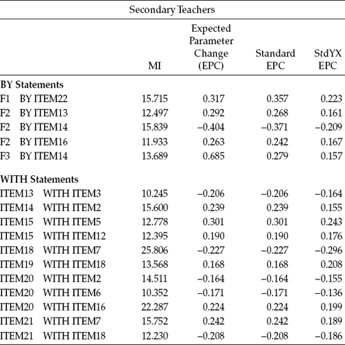
Although a review of the MI results in Table 7.4 reveals a few large values, here again, based on a moderately satisfactory goodness-of-fit (MLM χ²_[200] = 505.831; CFI = 0.937; RMSEA = 0.047; SRMR = 0.052) and bearing in mind the importance of model parsimony, I consider Model 4 as the final baseline model for secondary teachers. Comparison of these Model 4 results with those for Model 3 reveals the corrected difference to be statistically significant (ΔMLM χ²_[1] = 23.493, p < .001).

Having now established a separate baseline model for both elementary and secondary teachers, we are ready to test hypotheses bearing on the equivalence of the MBI across the two teaching panels. A pictorial representation of these baseline models is shown in Figure 7.1; it provides the foundation against which we test the series of increasingly stringent hypotheses related to MBI structure.

Table 7.4 Mplus Output for Model 4: Selected Modification Indices (MIs)

Testing Invariance: The Configural Model

Once the baseline models are established, the initial step in testing for invariance requires only that the same number of factors and the factor loading pattern be the same across groups. As such, no equality constraints are imposed on any of the parameters. Thus, the same parameters that were estimated in the baseline model for each group separately are again estimated in this multigroup model. In essence, then, you can think of the model tested here as a multigroup representation of the baseline models because it incorporates the baseline models for elementary and secondary teachers within the same file. In the SEM literature, this model is commonly termed the configural model (Horn & McArdle, 1992); relatedly, we can think of this step as a test of configural invariance.

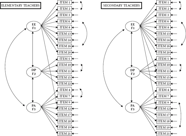
Figure 7.1. Hypothesized multigroup baseline model of MBI structure for elementary and secondary teachers.

From our work in determining the baseline models, and as shown in Figure 7.1, we already know a priori that there are three parameters (two residual covariances [Item 4 with Item 7; Item 9 with Item 19] and one cross-loading [Item 11 on F1]) that were not part of the originally hypothesized model and that differ across the two groups of teachers. However, over and above these group-specific parameters, it is important to stress that, although the originally hypothesized factor structure for each group is similar, it is not identical. Because no equality constraints are imposed on any parameters in the model in testing for configural invariance, no determination of group differences can be made. Such claims derive from subsequent tests for invariance to be described shortly.

Given that we have already conducted tests of model structure in the establishment of baseline models, you are no doubt wondering why it is necessary to repeat the process in this testing of the configural model. This multigroup model serves two important functions. First, it allows for invariance tests to be conducted across the two groups simultaneously. In other words, parameters are estimated for both groups at the same time. Second, in testing for invariance, the fit of this configural model provides the baseline value against which the first comparison of models (i.e., invariance of factor loadings) is made.⁵

Despite the multigroup structure of the configural and subsequent models, analyses yield only one set of fit statistics in the determination of overall model fit. When maximum likelihood (ML) estimation is used, the χ² statistics are summative, and, thus, the overall χ² value for the multigroup model should equal the sum of the χ² values obtained from separate testing of baseline models. In the present case, ML estimation of the baseline model for elementary teachers yielded a χ²₍₂₀₁₎ value of 545.846 and for secondary teachers a χ²₍₂₀₀₎ value of 643.964, we can expect a ML χ² value of 1189.81 with 401 degrees of freedom for the combined multigroup configural model. In contrast, when model estimation is based on the robust statistics, as they were in this application, the MLM χ² values are not necessarily summative across the groups.

Mplus Input File Specification and Output File Results

Input File 1

As there are several critically important points to be made in the use of Mplus in testing for multigroup invariance in general, as well as with our initial configural model, in particular, I now walk you through this first input file in order that I can elaborate on each of these new and key components of the file. In an effort to minimize confusion related to tests of invariance for several different models, each is assigned a different label, with this first model being labeled InvModel.1. The input file for this configural model is presented in Figure 7.2.

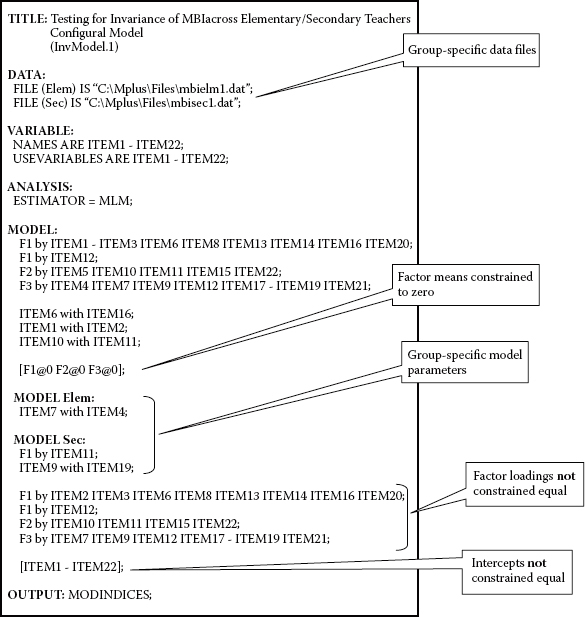
Figure 7.2. Mplus input file for test of configural model.

Before addressing the new model commands and specifications, let's first examine those portions of the file with which you are now familiar. As we review this input file, I highly recommend that you work from Figures 7.1 and 7.2 in combination, in order to more fully comprehend this first multigroup file structure.

As indicated in the VARIABLE command, there are 22 observed variables (ITEM1 through ITEM22), all of which are included in the analysis. The factors to which these variables are linked can be evidenced graphically from Figure 7.1. As we know from our work in Chapter 4, the data comprising MBI scores are nonnormally distributed. In light of this information, then, analyses are based on robust ML (MLM) estimation rather than on default ML estimation. Thus, we must specify our estimator choice via the ANALYSIS command. Turning next to the MODEL command, we observe only the pattern of factor loadings (lines 1–4) and residual covariances (lines 5–7) that were found to be the same across elementary and secondary teachers. The specification of these parameters represents those that will be tested for their invariance across the two groups. Finally, the OUTPUT command requests that MIs be included in the output file. Because I have not included the parenthesized value of 3.84 (the cutoff value for χ² with one degree of freedom at p = .05), only MIs with values greater than 10.00 will be reported.

Moving on to new aspects of the file, let's look first at the DATA command, where we find two FILE statements. When the data for each group reside in different files, Mplus requires a FILE statement specific to each group that provides a relevant label for the group and identifies the location of its data file. In the present case, as shown in Figure 7.2, we observe two FILE statements, the first one pertinent to elementary teachers and the other to secondary teachers. Note that each has been assigned a label (Elem; Sec), which appears within parentheses and precedes the word IS, followed by location of the related data file. It is imperative that each FILE statement include a group label as this information is needed in a later portion of the input file. Finally, Mplus considers the group associated with the first FILE statement to be Group 1; this designation is relevant when latent means are of interest (not the case here).

In contrast to the present application, but also of relevance, is how the multigroup input file is structured when the data for each group reside in the same file. Accordingly, in lieu of FILE statements, this situation requires use of the GROUPING option for the VARIABLE command. Determination of the group considered to be Group 1 is tied to the values of the grouping variable, with the group assigned the lowest value being Group 1. For example, given data grouping based on gender, with males assigned a grouping value of 0 and females a grouping value of 1, Mplus would consider males as Group 1. Finally, when analyses are based on summary data, the multigroup Mplus input file requires use of the NGROUPS option of the DATA command. For more details related to group data residing in a single file, and to summary data, readers are referred to Muthén and Muthén (2007–2010).

Let's move down now to the MODEL command and, in particular, to the specifications appearing within square brackets. Parameter specifications in the MODEL command for multigroup analyses, as for single-group analyses, hold for all groups. Thus, in reviewing specifications regarding the factor loadings and residual covariances earlier, I noted that only parameters that were similarly specified across groups were included in this overall model section.

Appearing below these specifications, however, you will see the following: [F1@0 F2@0 F3@0]. In Mplus, means (i.e., factor means), intercepts (i.e., observed variable means), and thresholds (of categorical observed variables) are indicated by their enclosure within square brackets. Relatedly, then, this specification indicates that the latent means of Factors 1, 2, and 3 are fixed at zero for both groups. The reason for this specification derives from the fact that in multigroup analysis, Mplus, by default, fixes factor means and intercepts to zero for the first group; these parameters are freely estimated for all remaining groups. This default, however, is relevant only when the estimation of latent factor means is of interest, which of course is not the case here. Thus, in structuring the input file for a configural model, it is necessary to void this default by fixing all factor means to zero, as shown in Figure 7.2.⁶

The next two MODEL commands are termed model-specific commands as each enables parameter specification that is unique to a particular group. Importantly, each of these (specific) MODEL commands must be accompanied by the group label used in the related FILE command. Failure to include this label results in an error message and no analysis being performed. Indeed, these two components of the input file are critical in specification of the correct multigroup model as they contain only parameters that differ from the overall MODEL command. Let's now take a closer look at their content, focusing first on parameter specifications contained within the first large bracket. Here, you will quickly recognize the specified residual covariance (Items 7 and 4) for elementary teachers (MODEL Elem:), and the one cross-loading covariance (Item 11 on Factor 1) and one residual covariance (Items 9 and 19) for secondary teachers (MODEL Sec:), as parameter specifications unique to each of their baseline models. As these parameters differ across the two groups, their invariance will not be tested. Thus, our tests for invariance necessarily invoke a condition of partial measurement invariance.

Turning to the next four lines of input appearing within the second bracket, you will recognize the same factor-loading parameters that appeared earlier under the initial overall (versus specific) MODEL command, with one exception—the first variable of each congeneric set is missing. Undoubtedly, you likely now are grappling with two queries concerning these specifications: (a) Why are these factor-loading specifications appearing again in this part of the input file, and (b) why is specification of the first variable for each factor not included?

The answer to the first query lies with the Mplus approach to specification of constraints in multigroup analyses and, in particular, with its related defaults. In CFA models based on continuous data, all factor loadings and intercepts are constrained equal across groups by default; in contrast, all residual variances are freely estimated by default. The technique for relaxing these defaulted constraints is to specify them under one of the MODEL-specific commands; this accounts for the replicated specification of only the common factor loadings here. Likewise, the same principle holds for the observed variable intercepts. Thus, because these parameters are also constrained equal across groups by default, they too need to be relaxed for the configural model. As noted earlier, means, intercepts, and thresholds are demarcated within square brackets. Accordingly, the specification of [ITEM1–ITEM22] requests that the observed variable intercepts not be constrained equal across groups.

The answer to the second query is tied to the issue of model specification. If you were to include Item 1 (for F1), Item 5 (for F2), and Item 4 (for F3), you would be requesting that these three parameters are free to vary for secondary teachers. The consequence of such specification would mean the model is underidentified.

In summary, the Mplus input file shown in Figure 7.2 is totally consistent with specification of a configural model in which no equality constraints are imposed. Model fit results derived from execution of this file therefore represent a multigroup version of the combined baseline models for elementary and secondary teachers. Results for this configural model (InvModel.1) were as follows: MLM χ²₍₄₀₁₎ = 958.341, CFI = 0.939, RMSEA = 0.047, and SRMR = 0.051.

Earlier in this chapter, I noted that when analyses are based on ML estimation, χ² values are summative in multigroup models. Although analyses here were based on MLM estimation, it may be of interest to observe that this summative information held true when the same analyses were based on ML estimation. Accordingly, results for the configural model yielded an overall χ²₍₄₀₁₎ value of 1189.811, which indeed represents a value equal to the summation of the baseline models for elementary teachers (χ²_[201] = 545.846) and secondary teachers (χ²_[200] = 643.964). Recall that the baseline model for secondary teachers comprised an additional cross-loading, which therefore accounts for the loss of one degree of freedom.

Testing Invariance: The Measurement Model

The key measurement model parameters of interest in the present application are the factor loadings and the commonly specified residual covariances. Details related to both the Mplus input file and analytic results are now presented separately for each.

Factor Loadings

As mentioned previously, in testing for the equivalence of factor loadings across groups, only those that are commonly specified for each group are of interest. Let's take a look now at Figure 7.3, where the input file for this multigroup model is shown, and see how it differs from that of the configural model. In reviewing this file, you will readily observe that the major difference between the two files lies with the absence of the additional four lines of factor-loading specifications that were previously listed under the MODEL-specific command for secondary teachers. Deletion of these specifications, which served to relax the equality constraints, thus allows the Mplus default regarding factor loadings to hold; that is, all factor loadings appearing in the overall MODEL command are constrained equal across the two groups of teachers. One additional change that I made to this input file was the parenthesized value of 3.84 accompanying the request for MIs in the OUTPUT file. As such, this value will be used as the cutpoint, rather than the usual value of 10.00, in the reporting of MI values. We'll label this factor-loading invariant model as InvModel.2.

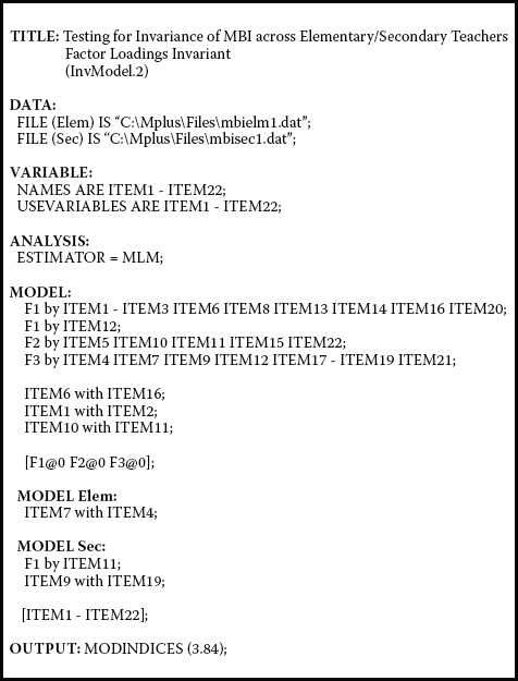
Figure 7.3. Mplus input file for test of invariant factor loadings.

Goodness-of-fit statistics related to InvModel.2 were MLM χ²₍₄₂₁₎ = 1015.228, CFI = 0.935, RMSEA = 0.047, and SRMR = 0.057. Note that the difference in degrees of freedom from the configural model is 20. This gain in the number of degrees of freedom, of course, derives from the fact that 19 factor loadings (excludes the reference variables that were fixed to 1.0) and 1 cross-loading were constrained equal across group. As indicated by the very slightly higher MLM χ² value and lower CFI value, compared with the configural model, results suggest that the model does not fit the data quite as well as it did with no factor-loading constraints imposed. Thus, we can expect to find some evidence of noninvariance related to the factor loadings. These results are presented in Table 7.5.

In reviewing results from this analysis, only the MIs related to the factor loadings are of interest, and, thus, only the BY statements are included in Table 7.5. An interesting feature of the Mplus output is that, in lieu of reporting MI results pertinent to the factor loadings in general, the program provides them for all groups involved in the analysis. In reviewing these MI values, you will quickly note that many of them represent factor-loading parameters that were not specified in the model. However, recall that the MIs bear only on parameters that are either fixed to zero or to some other nonzero value, or are constrained equal to other parameters in the model. In testing for invariance, only the latter are of relevance. In seeking evidence of noninvariance, however, we focus only on the factor loadings that were constrained equal across the groups. Of those falling into this category, we select the parameter exhibiting the largest MI value.⁷ As highlighted in Table 7.5, of all the eligible parameters, the factor loading of Item 11 on Factor 2 appears to be the most problematic in terms of its equivalence across elementary and secondary teachers.

Table 7.5 Mplus Output for Initial Test for Invariance of Factor Loadings: Selected Modification Indices (MIs) (InvModel.2)

Presented with this information, our next step is to modify the input file such that the parameter F2 by ITEM11 is freely estimated. As shown in the InvModel.1 input file, the relaxing of an equality constraint related to this factor loading is accomplished simply by specifying the parameter under one of the MODEL-specific commands. In the present case, I have included it under the MODEL-specific command for secondary teachers as shown in Figure 7.4. Importantly, however, this parameter remains specified under the general MODEL command; otherwise, it would not be estimated at all. This model is labeled InvModel.3.

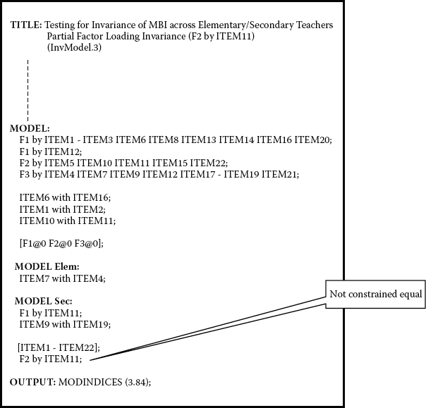
Figure 7.4. Mplus input file for test of partially invariant factor loadings.

Analysis of this partial invariance model resulted in a MLM χ² value of 989.427 with 420 degrees of freedom. (One additional parameter was estimated, thereby accounting for the loss of one degree of freedom.)⁸ The other fit indices were CFI = 0.938, RMSEA = 0.046, and SRMR = 0.054. A review of the estimated values of the relaxed parameter, F2 by ITEM11, for the two groups of teachers revealed a fairly substantial discrepancy, with the estimate for elementary teachers being 1.095 and for secondary teachers 0.581.

Of prime interest now is whether difference in model fit between this modified model (InvModel.3), in which the constraint on the loading of ITEM11 on F2 was relaxed, and the configural model (InvModel.1) is or is not statistically significant. To determine this information, given that analyses were based on MLM estimation, requires that we conduct a corrected chi-square difference test. This procedure, as I have noted previously, is available on the Mplus website (http://www.statmodel.com/chidiff.shtml).

Although I presented a walkthrough of this formula in Chapter 6, application in the case of invariance testing has a slightly different slant in that the second model represents the nested (i.e., more restrictive) model. Thus, I believe it would be helpful to you if I once again walk you through the computation of this difference test as it pertains to our first set of comparative models: that is, between the configural model and the current partially invariant model. For maximum comprehension of this computational work, I strongly suggest that you download the formula from the Mplus website in order that you can clearly follow all computations. Information you will need in working through this formula is as follows:

Configural model: Scaling correction factor = 1.242

Partially invariant model: Scaling correction factor = 1.239

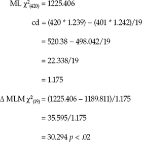
In checking this difference test result in the χ² distribution table, you will see that the value of 30.294 is just slightly over the cutpoint of 30.1435 for p < .05. Given this finding, we once again review the MIs for this model to peruse evidence of possibly additionally noninvariant factor loadings. These MI values are presented in Table 7.6. Of the four eligible candidates for further testing of invariance (F2 by ITEM5; F2 by ITEM15; F3 by ITEM7; F3 by ITEM17), the largest MI represents the loading of Item 15 on Factor 2.

As a consequence of this result we now return to InvModel.3 and modify it such that it now includes two freely estimated parameters (Items 11 and 15 on Factor 2); this model is labeled as InvModel.4. Goodness-of-fit results for this model were MLM χ²₍₄₁₉₎ = 981.189, CFI = 0.939, RMSEA = 0.046, and SRMR = 0.054. Estimates for the factor loading of Item 15 on Factor 2 were 0.683 for elementary teachers and 0.963 for secondary teachers. Finally, comparison of this model with the configural model yielded a corrected ΔMLM χ²₍₁₈₎ value of 21.975, which was not statistically significant (p > .05).

Table 7.6 Mplus Output for Test of Invariant Factor Loadings: Selected Modification Indices (MIs) for Partially Invariant Model (InvModel.3)

Residual Covariances

At this point, we know that all items on the MBI, except for Items 11 and 15, both of which load on Factor 2, are operating equivalently across the two groups of teachers. So now, let's move on to further testing of the invariance of this instrument. Of substantial interest are the three commonly specified residual covariances and the extent to which they may be invariant across the groups. Given that these residual covariances are not constrained equal by default, the process in specifying their invariance necessarily differs from the models analyzed thus far. The input file for this model (InvModel.5) is presented in Figure 7.5.

The only change in this model compared with the previous one is the parenthesized values of 1, 2, and 3, accompanying each of the three specified residual covariances. The assignment of these parenthesized numbers is indicative of the specification of equality constraints. The placement of each residual covariance and its accompanying parenthesized number (a) within the overall MODEL command and (b) on a separate line, ensures that each of these parameters will be constrained equal across the two groups and not to each other. Thus, an important caveat in specifying equality constraints in Mplus when the parameters of interest are not constrained equal by default is that only one constraint can be specified per line.

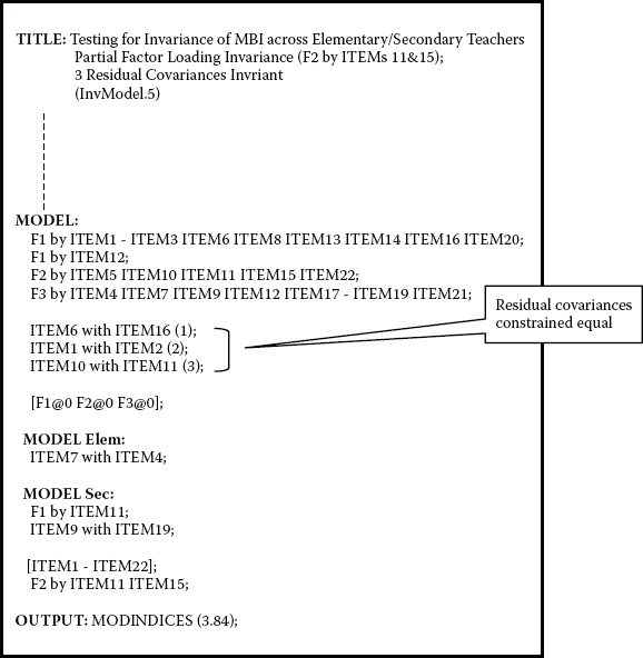
Figure 7.5. Mplus input file for test of invariant common residual covariances.

In total, 21 parameters in this model (InvModel.5) were constrained equal across groups: 17 factor loadings, 1 cross-loading, and 3 residual covariances. Model fit results deviated little from InvModel.4 and were as follows: MLM χ²₍₄₂₂₎ = 992.614, CFI = 0.938, RMSEA = 0.046, and SRMR = 0.054. Comparison of this model with the previous one (InvModel.4) representing the final model in the test for invariant factor loadings yielded a corrected ΔMLM χ²₍₃₎ value of 5.356, which was not statistically significant (p > .05), thereby indicating that specified residual covariances between Items 6 and 16, Items 1 and 2, and Items 10 and 11 are operating equivalently across elementary and secondary teachers.

Testing Invariance of the Structural Model

Having established invariance related to the measurement model, let's now move on to testing for the invariance of structural parameters in the model; these include only the factor variances and covariances in the present case.⁹ The input file for this model (InvModel.6) is presented in Figure 7.6.

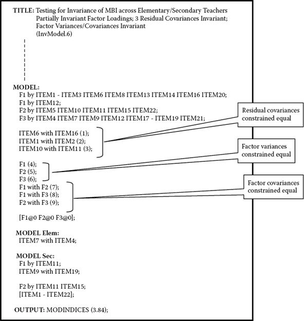
Figure 7.6. Mplus input file for test of invariant factor variances and covariances.

As you will readily note, consistent with the equality constraints pertinent to the three residual covariances, the factor variances and covariances are also not constrained equal by default and, thus, must be separately noted in the input file. Accordingly, equality constraints across groups for the factor variances are assigned the parenthesized values of 4 to 6, and those for the factor covariances 7 to 9. Note also that the item intercepts remain estimated as indicated by their specification within square brackets appearing under the MODEL-specific section for secondary teachers.

Goodness-of-fit results for the testing of InvModel.6 were MLMχ²₍₄₂₈₎ = 1004.731, CFI = 0.937, RMSEA = 0.046, and SRMR = 0.059. Comparison with InvModel.5 yielded a corrected difference value that was not statistically significant (ΔMLM χ²₍₆₎ = 12.165, p > 0.05). This information conveys the notion that, despite the presence of two noninvariant factor loadings, as well as the freely estimated item intercepts, the factor variances and covariances remain equivalent across elementary and secondary teachers. A summary of all noninvariant (i.e., freely estimated) unstandardized estimates is presented in Table 7.7.

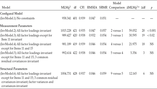
The primary focus of this first multigroup application was to test for the invariance of a measuring instrument across elementary and secondary teachers. However, because this application represented an initial overview of the invariance-testing process, it was purposely limited to the analysis of COVS only. As such, no tests for invariance of the observed variable intercepts and latent factor means were included. Details related to each step in the process were presented, the related Mplus input files reviewed, and relevant portions of the Mplus output files discussed. As is typically the case, these analyses resulted in the specification and testing of several different models. Thus, to facilitate your overview of these model results, as well as your understanding of the hierarchical process of invariance testing, a summary of all goodness-fit results, in addition to the ΔMLM χ² values, are presented in Table 7.8.

Table 7.7 Mplus Output: Noninvariant Parameters Across Elementary and Secondary Teachers

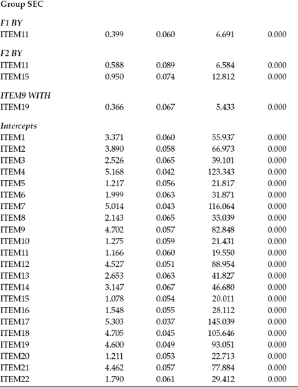
Table 7.8 Tests for Invariance of MBI Across Elementary and Secondary Teachers: Summary of Model Fit and χ²-Difference-Test Statistics

a Corrected values.

Notes

1.	For a detailed description of the MBI, readers are referred to Chapter 4 of the present volume.
2.	Middle-school teachers comprised the third group.
3.	As noted in Chapter 4, due to refusal of the MBI test publisher to grant copyright permission, I am unable to reprint the items here for your perusal. Nonetheless, a general sense of the item content can be derived from my brief descriptions of them in Chapter 4.
4.	All MLM chi-square difference results were based on corrected values calculated from the formula provided on the Mplus website (http://www.statmodel.com) and as illustrated in Chapter 6.
5.	Although it has become the modus operandi for researchers to compare adjacently tested models in computation of the χ2-difference test, one could also compare each increasingly restrictive model with the configural model, albeit taking into account the relevant increasing number of degrees of freedom.
6.	Although Mplus provides for a model option that negates the estimation of means intercepts, and thresholds (specified under the ANALYSIS command as MODEL = NOMEANSTRUCTURE), this option is not available with MLM (or MLMV, MLF, and MLR) estimation.
7.	Other eligible parameters are F2 by ITEM5, F2 by ITEM15, F2 by ITEM22, F3 by ITEM7, and F3 by ITEM17.
8.	In testing for invariance of the factor loadings (InvModel.2), the loading of Item 11 on F2 was freely estimated for Group 1 (elementary teachers), albeit constrained equal to this estimated value for Group 2 (secondary teachers). Thus, the loss of one degree of freedom arose from the additional estimation of this factor loading for secondary teachers.
9.	As noted earlier, although latent means are also considered to be structural parameters, they are not of interest in the present application.