chapter 8

Testing the Equivalence
of Latent Factor Means

Analysis of Mean and Covariance Structures

The multigroup application to be illustrated in this chapter differs from that of Chapter 7 in two major respects. First, analyses are based on mean and covariance structures (MACS), rather than on only covariance structures (COVS). Second, whereas the sample data are complete for one group, they are incomplete for the other. Prior to walking you through procedures related to this chapter's application, I present a brief review of the basic concepts associated with analyses of MACS, followed by the Mplus approach to analysis of missing data procedures.

Despite Sörbom's (1974) introduction of the MACS strategy in testing for latent mean differences over 30 years ago, a review of the structural equation modeling (SEM) literature reveals only a modicum of studies to have been designed in testing for latent mean differences across groups based on real (as opposed to simulated) data (see, e.g., Aikin, Stein, & Bentler, 1994; Byrne, 1988b; Byrne and Stewart, 2006; Cooke, Kosson, & Michie, 2001; Little, 1997; Marsh & Grayson, 1994; Reise, Widaman, & Pugh, 1993; Widaman & Reise, 1997). The focus in this chapter is to test for the invariance of latent means across two different cultural groups. The present application is taken from a study by Byrne and Watkins (2003) but extends this previous work in two ways: (a) Analyses are based on MACS, rather than on only COVS; and (b) analyses address the issue of missing data with respect to the Nigerian sample, albeit data are complete for the Australian sample.

Testing Latent Mean Structures: The Basic Notion

In the usual univariate or multivariate analyses involving multigroup comparisons, one is typically interested in testing whether the observed means representing the various groups are statistically significantly different from each other. Because these values are directly calculable from the raw data, they are considered to be observed values. In contrast, the means of latent variables (i.e., latent constructs) are unobservable; that is, they are not directly observed. Rather, these latent constructs derive their structure indirectly from their indicator variables, which, in turn, are directly observed and hence measurable. Testing for the invariance of mean structures, then, conveys the notion that we intend to test for the equivalence of means related to each underlying construct or factor. Another way of saying the same thing, of course, is that we intend to test for latent mean differences between or among the groups under study.

For all the examples considered thus far, analyses have been based on COVS rather than on MACS. As such, only parameters representing regression coefficients, variances, and covariances have been of interest. Accordingly, because covariance structure of the observed variables constitutes the crucial parametric information, a hypothesized model can thus be estimated and tested via the sample covariance matrix. One limitation of this level of invariance is that whereas the unit of measurement for the underlying factors (i.e., the factor loading) is identical across groups, the origin of the scales (i.e., the intercepts) is not.¹ As a consequence, comparison of latent factor means is not possible, thereby leading Meredith (1993) to categorize this level of invariance as “weak” factorial invariance. This limitation, notwithstanding evidence of invariant factor loadings, nonetheless permits researchers to move on in testing further for the equivalence of factor variances, factor covariances, and the pattern of these factorial relations, a focus of substantial interest to researchers interested more in construct validity issues than in testing for latent mean differences. These subsequent tests would continue to be based on the analysis of COVS as illustrated in Chapter 7.

In contrast, when analyses are based on MACS, the data to be modeled include both the sample means and the sample covariances. This information is typically contained in a matrix termed a moment matrix. The format by which this moment matrix is structured, however, varies across SEM programs.

In the analysis of COVS, it is implicitly assumed that all observed variables are measured as deviations from their means; in other words, their means are equal to zero. As a consequence, the intercept terms generally associated with regression equations are not relevant to the analyses. However, when the observed means take on nonzero values, the intercept parameter must be considered, thereby necessitating a reparameterization of the hypothesized model. Such is the case when one is interested in testing for the invariance of latent mean structures. The following example (see Bentler, 2005) may help to clarify both the concept and the term mean structures. Consider first the following regression equation:

y = α + βx + ε

(8.1)

where α is an intercept parameter. Although the intercept can assist in defining the mean of y, it does not generally equal the mean. Thus, if we now take expectations of both sides of this equation and assume that the mean of ε is zero, the above expression yields

μ_y = α + βμ_x

(8.2)

where μ_y is the mean of y, and μ_x is the mean of x. As such, y and its mean can now be expressed in terms of the model parameters α, β, and μ_x. It is this decomposition of the mean of y, the dependent variable, that leads to the term mean structures. More specifically, it serves to characterize a model in which the means of the dependent variables can be expressed or “structured” in terms of structural coefficients and the means of the independent variables. The above equation serves to illustrate how the incorporation of a mean structure into a model necessarily includes the new parameters α and μ_x, the intercept and observed mean (of x), respectively. Thus, models with structured means merely extend the basic concepts associated with the analysis of covariance structures.

In summary, any model involving mean structures may include the following parameters:

• Regression coefficients (i.e., the factor loadings)
• Variances and covariances of the independent variables (i.e., the factors and their residuals)
• Intercepts of the dependent variables (i.e., the observed measures)
• Means of the independent variables (i.e., the factors)

Model Parameterization

As with the invariance application presented in Chapter 7, applications based on structured means models involve testing simultaneously across two or more groups. However, in testing for invariance based on the analysis of MACS, testing for latent mean differences across groups is made possible through the implementation of two important strategies—model identification and factor identification.

Model Identification

Given the necessary estimation of intercepts associated with the observed variables, in addition to those associated with the unobserved latent constructs, it is evident that the attainment of an overidentified model is possible only with the imposition of several specification constraints. Indeed, it is this very issue that complicates, and ultimately renders impossible, the estimation of latent means in single-group analyses. Multigroup analyses, on the other hand, provide the mechanism for imposing severe restrictions on the model such that the estimation of latent means is possible. More specifically, because two (or more) groups under study are tested simultaneously, evaluation of the identification criterion is considered across groups. As a consequence, although the structured means model may not be identified in one group, it can become so when analyzed within the framework of a multigroup model. This outcome occurs as a function of specified equality constraints across groups. More specifically, these equality constraints derive from the underlying assumption that both the observed variable intercepts and the factor loadings are invariant across groups. Nonetheless, partial measurement invariance pertinent to both factor loadings and intercepts can and does occur. Although, in principle, testing for the equivalence of latent mean structures can involve partial measurement invariance related to the factor loadings, the intercepts, or both, this condition can lead to problems of identification, which will be evidenced in the present application.

Factor Identification

This requirement imposes the restriction that the factor intercepts for one group be fixed to zero; this group then operates as a reference group against which latent means for the other group(s) are compared. The reason for this reconceptualization is that when the intercepts of the measured variables are constrained equal across groups, this leads to the latent factor intercepts having no definite origin (i.e., they are undefined in a statistical sense). A standard way of fixing the origin, then, is to set the factor intercepts of one group to zero (see Bentler, 2005; Jöreskog & Sörbom, 1996; Muthén & Muthén, 2007–2010). As a consequence, factor intercepts are interpretable only in a relative sense. That is to say, one can test whether the latent variable means for one group differ from those of another, but one cannot estimate the mean of each factor in a model for each group. In other words, although it is possible to test for latent mean differences between, say, college men and women, it is not possible to estimate, simultaneously, the mean of each factor for both men and women; the latent means for one group must be constrained to zero.

The Testing Strategy

The approach to testing for differences in latent factor means follows the same pattern that was outlined and illustrated in Chapter 7. That is, we begin by first establishing a well-fitting baseline model for each group separately. This step is followed by a hierarchically ordered series of analyses that test for the invariance of particular sets of parameters across groups.

The primary difference in the tests for invariance in Chapter 7 (based on the analysis of COVS) and those based on the analysis of MACS in this chapter is the additional tests for the equivalence of intercepts and latent factor means across groups. We turn now to the hypothesized model under study and the related tests for invariance of a first-order CFA structure.

The Hypothesized Model

The application examined in this chapter bears on the equivalency of latent mean structures related to four nonacademic self-concept (SC) dimensions—Physical Self-Concept (PSC: Appearance), Physical SC (PSC: Ability), Social SC (SSC: Peers), and Social SC (SSC: Parents)—across Australian and Nigerian adolescents. These constructs comprise the four nonacademic SC components of the Self-Description Questionnaire I (SDQ-I; Marsh, 1992). Although the data for Australian adolescents are complete (n = 497), those for Nigerian adolescents (n = 463) are incomplete.

Analyses of these data in the Byrne and Watkins (2003) study yielded evidence of substantial multivariate kurtosis.² In contrast to use of the robust maximum likelihood (MLM) estimator used with previous analyses of nonnormally distributed data (see Chapters 4, 6, and 7), in this chapter we use the robust maximum likelihood (MLR) estimator, the χ² statistic, considered asymptotically equivalent to the Yuan-Bentler (Y-B χ²; 2000) scaled statistic (Muthén & Muthén, 2007–2010). The Y-B χ² is analogous to the S-B χ² (i.e., the MLM estimator in Mplus) when data are both incomplete and nonnormally distributed, which is the case in the present application. Finally, as with the item score data in Chapter 7, SDQ-I responses are analyzed here as continuous data. However, for readers interested in testing for invariance based on ordered-categorical data, I highly recommend the Millsap and Yun-Tein (2004) article in which they addressed the problematic issues of model specification and identification commonly confronted when data are of a categorical nature. Also recommended, albeit more as a guide to these analyses when based on Mplus, is a web note by Muthén and Asparouov (2002) that is available through the program's website (http://www.statmodel.com).

The originally hypothesized model of SDQ-I factorial structure, tested separately for each group, is presented schematically in Figure 8.1.

Testing Multigroup Invariance

As noted in Chapter 7 and earlier in this chapter, the first step in testing for multigroup invariance is to establish an acceptably well-fitting baseline model for each group of interest. In the present case, we test for the invariance of factor loadings, intercepts, and latent factor means related to the four nonacademic SC scales of the SDQ-I across Australian and Nigerian adolescents.

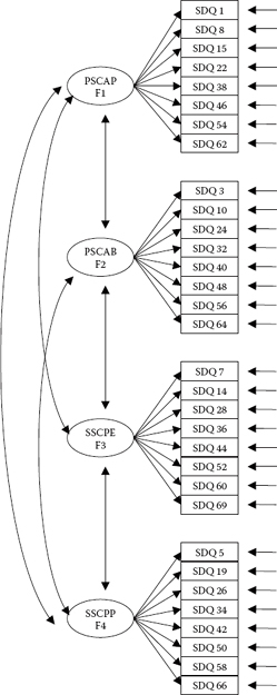
Figure 8.1. Hypothesized model of factorial structure for the Self-Description Questionnaire-I (SDQ-I; Marsh, 1992).

Establishing Baseline Models: Australian and Nigerian Adolescents

Australian Adolescents

Initial testing of the hypothesized model for this group yielded a MLR χ²₍₄₅₈₎ value of 1135.488, with results from the other robust fit indices conveying mixed messages regarding model fit. Whereas the CFI suggested a very poor fit to the data (CFI = 0.882), the RMSEA and SRMR results (0.055 and 0.065, respectively) revealed model fit that could be considered relatively good. A review of the modification indices (MIs) revealed several large values, with the MI for a residual covariance between SDQ40 (I am good at sports) and SDQ24 (I enjoy sports and games) exhibiting the largest value. As discussed in several chapters in this book, such covariance can result from overlapping item content, which appears to be the case here. Thus, Model 2 was specified in which this parameter was freely estimated. Although the (corrected) difference value between the initially hypothesized model (Model 1) and Model 2 was statistically significant, improvement in model fit was minimal (χ²_[457] = 1067.972; CFI = 0.893; RMSEA = 0.052 ; SRMR = 0.066).

Subsequent testing that included decreasingly restrictive parameter respecifications resulted in a baseline model considered to be the most appropriate in representing the data for Australian adolescents. This final model incorporated three additional parameters: (a) the cross-loading of SDQ38 (Other kids think I am good looking) on Factor 3 (SSC: Peers), (b) a residual covariance between SDQ26 (My parents like me) and SDQ19 (I like my parents), and (c) the cross-loading of SDQ32 (I have good muscles) on Factor 1 (PSC: Appearance). Whereas the underlying rationale in support of the first two respecifications was reasonably clear, the cross-loading of SDQ32 on Factor 1 seemed more tenuous as it suggested possible gender specificity. Nonetheless, two aspects of these results argued in favor of inclusion of this latter parameter: (a) the substantial size of its MI value compared with those of remaining parameters, and (b) misspecification regarding this parameter replicated for Nigerian adolescents. Model fit for this baseline model was as follows: MLRχ²₍₄₅₄₎ = 908.335, CFI = 0.921, RMSEA = 0.045, and SRMR = 0.056.

Admittedly, goodness-of-fit related to this baseline model for Australian adolescents can be considered only moderately acceptable, at best, at least in terms of the CFI. Although MI results suggested several additional parameters that, if included in the model, would improve fit substantially, the rationale and meaningfulness of these potential respecifications were difficult to defend. Coupled with these latter findings is the reality that in multiple-group SEM, the less parsimonious a model (i.e., the more complex it is as a consequence of the inclusion of additional parameters), the more difficult it is to achieve group invariance. As a consequence, the researcher walks a very thin line in establishing a sufficiently well-fitting yet sufficiently parsimonious model. These raisons d’être, then, together with recommendations by some (e.g., Cheung, Leung, & Au, 2006; Rigdon, 1996) that the RMSEA may be a better measure of model fit than the CFI under certain circumstances, stand in support of the baseline model for Australian adolescents presented here.

Nigerian Adolescents

Given the incomplete nature of SDQ-I responses for these adolescents, it was necessary that missingness be addressed in analyses of the data. Although there are many approaches that can be taken in dealing with missing data, the one that has been considered the most efficient and therefore the most highly recommended, for at least the last decade or so, is that of maximum likelihood (ML) estimation (see, e.g., Arbuckle, 1996; Enders & Bandalos,2001; Gold & Bentler, 2000; Schafer & Graham, 2002). Nonetheless, Bentler (2005) noted that when the amount of missing data is extremely small, there may be some conditions where some of the more commonly used methods such as listwise and pairwise deletion, hot deck, and mean imputation may suffer only marginal loss of accuracy and efficiency compared with the ML method pairwise. (For an abbreviated review of the issues, advantages, and disadvantages of various approaches to handling missing data, readers are referred to Byrne, 2009. For a more extensive and comprehensive treatment of these topics, see Arbuckle, 1996; Enders, 2010; Schafer & Graham, 2002. For a comparison of missing data methods, see Enders & Bandalos, 2001. And for a review of ML methods, see Enders, 2001.)

Mplus provides for many different options regarding the estimation of models with incomplete data. These choices vary in accordance with type of missingness, type of variables (continuous, categorical [ordered and unordered], counts, binary, censored, or any combination thereof), and type of distribution, be it normal or nonnormal (Muthén & Muthén, 2007–2010). In addition, Mplus enables multiple imputation of missing data using Bayesian analyses. (For a general overview of this Bayesian procedure, see Rubin, 1987; Schafer, 1997. For application within the framework of Mplus, see Asparouov & Muthén, 2010; Muthén, 2010.)

As noted earlier in this chapter, given the presence of incomplete data for Nigerian adolescents, in addition to the fact that data for both groups are known to be nonnormally distributed, all analyses are based on the MLR estimator, which can take both issues into account as it is analogous to the Y-B χ² (Yuan & Bentler, 2000). Prior to analyses focused on establishment of the baseline model for these adolescents, I considered it important first to conduct a descriptive analysis of these data in order to determine the percentage and pattern of missing data. This task is easily accomplished either by specifying TYPE=BASIC in the ANALYSIS command, or by requesting the option PATTERNS in the OUTPUT command. The only difference between the two specifications is that whereas the former specification additionally yields information related to the observed variable means and standard deviations, the latter specification does not.

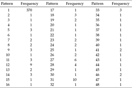
Let's now review the Mplus output file as it bears on these missing data. Presented in Table 8.1 is the usual summary information pertinent to this analysis. Of particular relevance here is that the number of observations is 463, whereas the number of missing data patterns is 48. A summary of these data patterns is shown in Table 8.2, with the numbered heading of each column identifying one pattern and each x representing a data point that is not missing. Finally, in Table 8.3, we find a summary of frequencies related to each missing data pattern. By combining information from Tables 8.2 and 8.3, for example, we are advised that for Pattern 5, three persons failed to respond to the Item SDQ62. In a second example, only one case was linked to Pattern 48, which was shown to have missing data for Items SDQ22, SDQ24, SDQ26, SDQ52, and SDQ66.

Table 8.1 Mplus Output: Selected Summary Information

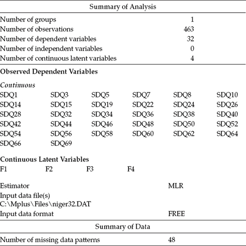
Table 8.2 Mplus Output: Summary of Missing Data Patterns

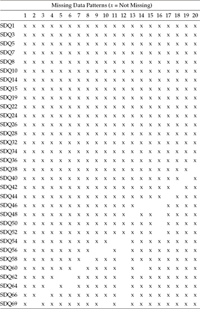
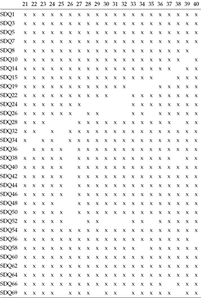
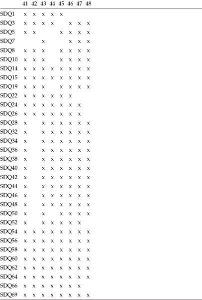
Table 8.3 Mplus Output: Missing Data Pattern Frequencies

Let's return now to findings related to testing of the hypothesized model for Nigerian adolescents. In contrast to the Australian group, results revealed a substantially better fitting model, albeit still only marginally acceptable, at least in terms of the CFI (MLRχ²_[458] = 726.895; CFI = 0.913; RMSEA = 0.036; SRMR = 0.052). A review of the MI values identified one parameter, in particular, that could be regarded as strongly misspecified; this parameter represented an error covariance between Items 26 and 19, which, of course, replicates the same finding for Australian adolescents. In addition, however, the MI results identified the same two cross-loadings reported for the Australian groups (F3 by SDQ38; F1 by SDQ32), as well as other moderately misspecified parameters in the model. These three parameters were each separately added to the model, and then the model was reestimated. In the interest of space, however, only results for the final model that included all three parameters are reported here. Accordingly, results led to some improvement in fit such that the model could now be regarded as moderately good (MLRχ²_[455] = 665.862; CFI = 0.932; RMSEA = 0.032; SRMR = 0.047). Given no further evidence of misspecified parameters, this model was deemed the most appropriate baseline model for Nigerian adolescents.

Having established a baseline model for both groups of adolescents, we can now proceed in testing for the invariance of factor loadings, intercepts, and latent factor means across the two groups. These baseline models are schematically presented in Figure 8.2, with the broken lines representing additional parameter specifications common to both Australians and Nigerians.

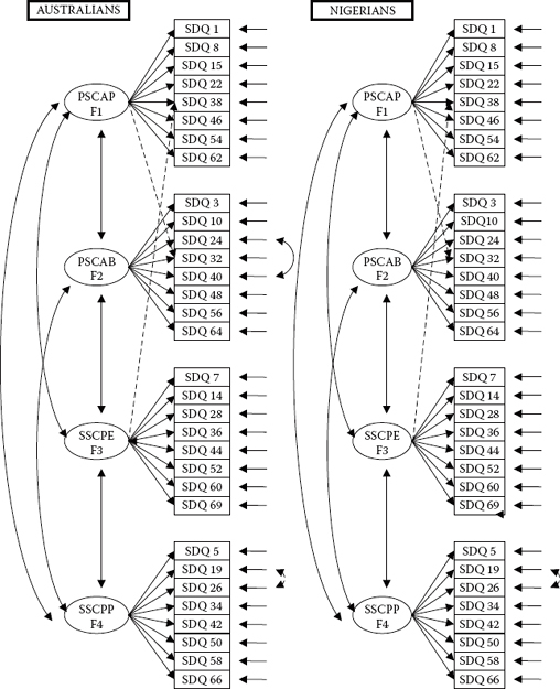
Figure 8.2. Baseline models of SDQ-I structure for Australian and Nigerian adolescents.

Mplus Input File Specification and Output File Results

Testing Invariance: The Configural Model

Input File 1

As noted in Chapter 7, the model under test in this step of the invariance-testing process is a multigroup model in which no parameter constraints are imposed. The configural model simply incorporates the baseline models pertinent to both groups and allows for their simultaneous analyses. The input file for this initial model is shown in Figure 8.3.

At first blush, you may assume that this file essentially mimics the same structure as that for the configural model in Chapter 7. Although this is basically true, one major difference between the two files is that I addressed the issue of model identification and latent variable scaling using the fixed factor, rather than the Mplus default reference variable method. (For a review of these methods in general, together with their related references, see Chapter 2; for a perspective on use of the reference variable approach as it relates to invariance testing in particular, see Yoon & Millsap, 2007.) Specification pertinent to the fixed factor method can be evidenced under the primary MODEL command and involves two adjustments to the usual default. First, note that the first variable of each congeneric set per factor is freely estimated, as indicated by the accompanying asterisk (*). In all previous input files, with the exception of Chapter 5, specification has allowed the Mplus default to hold, thereby fixing the value of these variables to 1.00. Second, given the free estimation of these initial variables in each congeneric set, the related factor variance must be fixed to 1.00, as indicated by the specification of F1–F4@1.

Inspection of specifications for both the factor loadings and residual covariance in the MODEL command reveals the similarity of the two baseline models. The only hypothesized difference between the two groups lies with the specification of the residual covariance of SDQ40 with SDQ24 for Australian adolescents.

Consistent with the configural model specifications noted in Chapter 7, the factor loadings are freely estimated for both adolescent groups. Thus, to offset the defaulted equality constraint for these factor-loading parameters, their specifications are repeated under the MODEL-specific command for Nigerian adolescents. Finally, note that the factor means are fixed at 0.0 ([F1–F4@0]) and the observed variable intercepts not estimated ([SDQ1–SDQ69]).

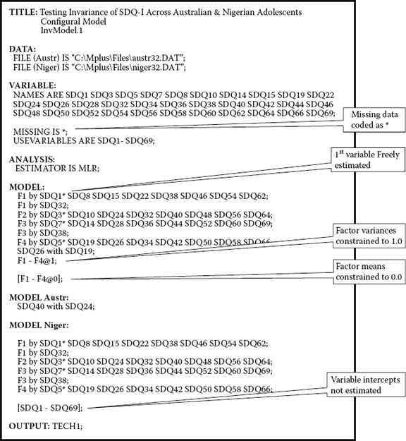
Figure 8.3. Mplus input file for a test of a configural model.

Not surprisingly, results from testing of the configural model yielded goodness-of-fit statistics that were moderately acceptable (MLRχ²_[909] = 1575.474). Indeed, the minimally acceptable CFI value of 0.924 was offset by the relatively good RMSEA and SRMR values of 0.039 and 0.052, respectively.

Testing Invariance: The Factor Loadings

As discussed and illustrated in Chapter 7, our next step in the invariance-testing process is to now constrain all the factor loadings equal across the two groups. Specification of this model requires that the replicated list of common factor loadings under the MODEL-specific command for the second group (in this case, for MODEL Niger;) be deleted. (For comparison, see Figure 7.3.) Removal of these parameter specifications then allows for the Mplus default of factor-loading equality to hold.

Recall that in reviewing the MI values pertinent to these constraints, we focus on only those that are (a) related to the factor-loading matrix, and (b) actually constrained equal across groups. As such, only the BY statements are of interest here. Indeed, you may wonder why I bother to note point (b) above. The reason for this alert is because many additional factor-loading parameters will also be included in this set of MIs and can be confusing for those new to the Mplus program. These other MI values, of course, simply suggest other parameters that if incorporated into the model would lead to a better model fit. However, our determination of best fitting models was completed with the establishment of appropriate baseline models, and thus further model fitting is not relevant here. Findings from this initial test for parameter equality identified the loading of SDQ24 on F2 as having the largest MI value, thereby indicating the severity of its noninvariance across Australian and Nigerian adolescents. Goodness-of-fit results for this model are as follows: MLRχ²₍₉₄₃₎ = 1744.821, CFI = 0.909, RMSEA = 0.042, and SRMR = 0.093. Indeed, the notable decrease in model fit compared with that of the configural model provides clear evidence of extant noninvariance in this model. This fact is further substantiated by the very large corrected MLRχ²₍₃₄₎ difference value of 168.681, with 34 degrees of freedom relating to the 32 initial factor loadings plus 2 cross-loadings common to each group.

Before moving on with further testing of these factor loadings, allow me to digress briefly in order to provide you with one caveat and one recommendation regarding these analyses. We turn first to the caveat. Although, admittedly, I have mentioned this caution at various stages throughout the book, I consider it important to again alert you to the fact that because the calculation of MI values is done univariately, the values can fluctuate substantially from one test of the model to another. For this reason, then, it is imperative that only one constraint be relaxed at a time and the model reestimated after each respecification. As for my recommendation, I highly suggest, particularly to those who may be new to SEM, that the TECH1 option be included on the initial execution of each set of invariance tests as it serves as a check that you have specified the model correctly. For example, in this initial test of the factor loadings, the TECH1 output reveals the numbering of estimated parameters in the factor-loading matrix to extend from 33 to 65 for the first group (in this case, the Australians). Given that these parameters are specified as being constrained equal across groups, these parameters should be likewise numbered for the Nigerians.

Continued testing for the equality of SDQ factor loadings across groups identified six additional ones to be noninvariant. In total, the seven items found to be operating nonequivalently across groups were as follows:

• SDQ24 (I enjoy sports and games) on F2

• SDQ40 (I am good at sports) on F2

• SDQ26 (My parents like me) on F4

• SDQ19 (I like my parents) on F4

• SDQ38 (Other kids think I am good looking) on F1

• SDQ52 (I have more friends than most other kids) on F3

• SDQ22 (I am a nice-looking person) on F1

The input file for this final model designed to test for factor-loading invariance is shown in Figure 8.4. Of relevance is the specification of these seven noninvariant factor loadings under the MODEL-specific command for the Nigerian group. Their specification here assures that they are not constrained equal across the two groups. Of particular note from these analyses also is the verified invariance of the two cross-loadings across Australian and Nigerian adolescents (F1 by SDQ32; F3 by SDQ38).

Goodness-of-fit statistics related to this final model are as follows: MLRχ²₍₉₃₆₎ = 1646.326, CFI = 0.919, RMSEA = 0.040, and SRMR = 0.084. Comparison of this final model having equality constraints released for seven factor loadings with the previously specified model (with six factor loadings constrained equal) yielded a corrected MLRΔχ²₍₁₎ value of 4.548 (p < 0.020). Although this value slightly exceeds the χ² distribution cut-point of 3.84, its z-value is nonetheless less than 1.96. Also of relevance is the difference in CFI values, which is 0.01.³

Testing Invariance: The Common Residual Covariance

Input File 2

As noted in Chapter 7, testing for the invariance of error covariance is considered to be extremely stringent and really unnecessary (see, e.g., Widaman & Reise, 1997). Nonetheless, given that the error covariance between Item 26 and Item 19 was found to be an important parameter in the baseline model for both Australian and Nigerian adolescents, I consider it worthwhile, from a psychometric perspective, to test for its invariance across the two groups. Given that these two parameters were already freely estimated for each group, we simply need to indicate their equality constraint by adding a parenthesized 1 to their model specification as shown in Figure 8.5. (For a more detailed explanation regarding this form of imposing equality constraints, see Chapter 7.)

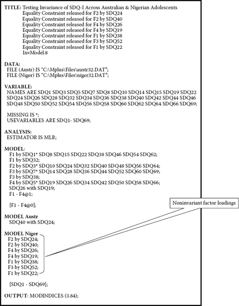
Figure 8.4. Mplus input file for a final test of invariant factor loadings.

Results related to the testing of this model yielded an ever so slightly better fit to the data than was the case for the previous model, in which only seven factor loadings were constrained equal (MLRχ²_[937] = 1644.489; CFI = 0.920; RMSEA = 0.040; SRMR = 0.084). The corrected difference test between these two models yielded as MLRΔχ²_m = 0.279, which, of course, is not statistically significant (p > .05). Thus, whereas the factor loadings for items SDQ26 (My parents like me) and SDQ19 (I like my parents), both of which load on F4, were found not to be invariant across Australian and Nigerian adolescents, the covariance between their residual terms was strong. What can we conclude from this rather intriguing finding? One suggestion is that although perception of content related to these items would appear to vary across the cultural groups (e.g., the type of parental relations that adolescents in each culture consider to be important), the degree of overlap between the content of the items is almost the same.

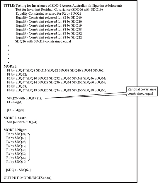
Figure 8.5. Mplus input file for a test of invariant common residual covariance.

Testing Invariance: The Intercepts

Input File 3

To recapitulate the current invariance-testing status of the SDQ-I thus far, we have found all factor loadings except those for seven items (SDQ24, SDQ40, SDQ26, SDQ19, SDQ38, SDQ52, and SDQ22), the two cross-loadings (SDQ32 on F1; SDQ38 on F3), and the residual covariance of SDQ26 with SDQ19 to be operating equivalently across Australian and Nigerian adolescent groups. In continuing these tests for measurement invariance, we next add the observed variable intercepts to the existing model. The partial input file for this new model is shown in Figure 8.6.

Recall that, in multigroup models, Mplus constrains intercepts of the observed variables equal across groups by default. In order to relax this constraint for the previous models, these parameters were specified within square brackets and entered under the MODEL-specific section for Nigerian adolescents. Given our focus now on testing for the invariance of these 32 SDQ-I item intercepts, however, this bracketed information has been deleted.

Results from analysis of this model were MLRχ²₍₉₆₉₎ = 2327.916, CFI = 0.846, RMSEA = 0.054, and SRMR = 0.128. Even before looking at the MIs, it seems evident that this model is critically less well fitting than any of the previous models tested thus far. Thus, it seems apparent that there is likely to be substantial evidence of noninvariance of the intercepts. Indeed, comparison of this model with the previous model (seven freely estimated factor loadings, and one residual covariance constrained equal) yielded a corrected ΔMLRχ²₍₃₂₎ value of 841.269(p < 0.001).

Not surprisingly, examination of the MIs for this model (see Table 8.4) revealed several extremely large values, with the value for SDQ7 being the largest (MI = 56.864). Testing of a subsequent model, in which the intercept for SDQ7 was freely estimated, yielded the following goodness-of-fit indices: MLRχ²₍₉₆₈₎ = 2264.088, CFI = 0.853, RMSEA = 0.053, and SRMR = 0.128. Once again, in comparing this model with the first model testing for invariant intercepts, the difference test revealed an extremely high and, of course, statistically significant corrected ΔMLRχ²₍₁₎ value of 283.752 (p < 0.001).

In total, continuation of these tests for invariance revealed 27 of the 32 intercepts to be nonequivalent across the two groups. Recall that because Mplus constrains the intercepts equal across groups by default, relaxation of these constraints requires that specification of nonequivalent intercepts be specified under the model-specific command for one of the groups (the Nigerians here). Thus, a review of these 27 nonequivalent intercepts can be seen in the input file for this final model as presented, in part, in Figure 8.7. Results bearing on this final model were as follows: MLRχ²₍₉₄₂₎ = 1649.972, CFI = 0.919, RMSEA = 0.040, and SRMR = 0.082. Comparison of this final model (equality constraints released for 27 intercepts) with the previously specified model (equality constraints released for 26 intercepts) yielded a corrected MLRΔχ²₍₁₎ value of 4.825 (p < 0.020). Consistent with results for the factor loadings, this value slightly exceeds the χ² distribution cutpoint of 3.84. However, given that its z-value is less than 1.96 and there is virtually no difference in CFI values (i.e., both are 0.919), I considered this model to represent appropriately the final test of intercepts related to the SDQ-I.

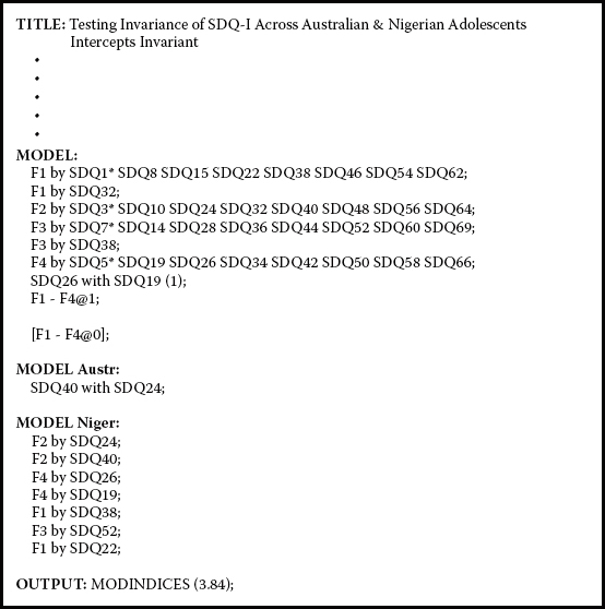
Figure 8.6. Mplus input file for a test of invariant observed variable intercepts.

Testing Invariance: The Latent Means

Input File 4

As mentioned in this chapter, tests for the invariance of latent means are more commonly expressed as tests for latent mean differences. Recall also from earlier discussion of identification issues that because the latent factor intercepts (i.e., factor means) have an arbitrary origin when intercepts of the observed variables are constrained equal, the latent factor means for one group must be fixed to zero, whereas those for the other group are freely estimated. As such, one group operates as the reference group against which the other group is compared. It is important to note, however, that Mplus automatically fixes the factor mean for the first group to zero by default (the Australian group in the present application). Given findings of noninvariance related to 7 factor loadings and 27 observed variable intercepts, our test for latent mean differences represents a partially invariant model. The input file for this test is shown, in part, in Figure 8.8.

Table 8.4 Mplus Output: Selected Modification Indices (MIs) for Test of Invariant Intercepts

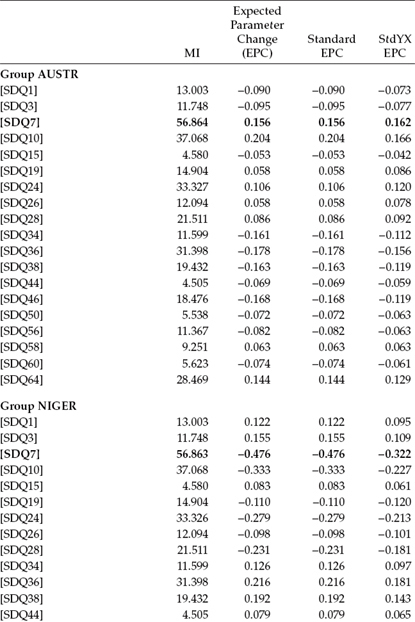
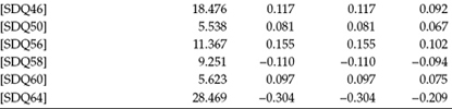
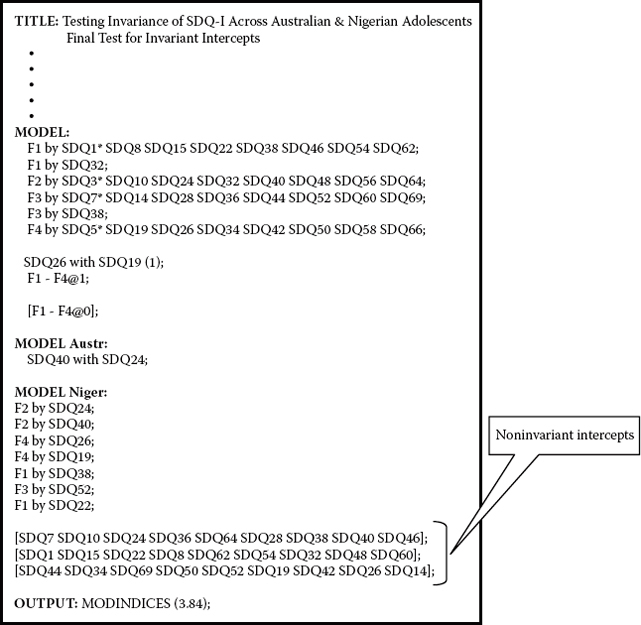
Figure 8.7. Mplus input file for a final test of invariant observed variable intercepts.

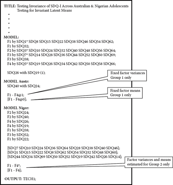
Figure 8.8. Mplus input file for a test of invariant latent means.

Figure 8.9. Mplus error message suggesting possible underidentification.

Review of this input file triggers several points worthy of mention. First, in contrast to all previous invariance models whereby the constraint, (F1–F4@1), was specified under the MODEL command, this specification has now been reassigned to the MODEL-specific command for the first group (Australians). Second, although the program fixes the factor mean to zero by default for this first group, as noted in this chapter, I prefer to override this default here in the interest of making this specification more explicit. Third, under the MODEL-specific command for the Nigerians, note that the specification of 7 factor loadings and 27 intercepts identifies those parameters as noninvariant, thereby allowing them to be freely estimated. Finally, also under MODEL Niger, you will see that for this group, the factor variances are freely estimated, as are the four factor means.

Execution of this file resulted in the condition code and related warning shown in Figure 8.9, which notes that the robust chi-square statistic could not be computed. As a result, of course, no goodness-of-fit statistics were reported. This warning message suggests that the model may not be identified. Indeed, given the number of freely estimated intercepts as a consequence of their noninvariance, this caveat is likely to be true as the model may be underidentified. (For an explanatory description of identification, see Chapter 2.)

Of import here is a critical criterion requiring the number of estimated intercepts to be less than the number of measured variables in the analysis of MACS models. In multigroup models, this requirement is controlled by the imposition of equality constraints across the groups. However, when these models incorporate partial measurement invariance, this balance between constrained and estimated parameters can become somewhat tenuous. Thus, it behooves us at this point to determine if, in fact, we have satisfied this criterion. The status of these parameters is as follows:

• Intercepts: 27 noninvariant, which translates into 27 estimated for each group (i.e., 54)

• 5 invariant intercepts—therefore 5 estimated

• Total number of intercepts freely estimated—59 (54+5)

• Factor loadings: 7 noninvariant, translating into 7 estimated for each group (i.e., 14)

• 25 invariant factor loadings—therefore 25 estimated

• 2 invariant cross-loadings—therefore 2 estimated

• Total number of factor loadings freely estimated = 41 (14 + 25 + 2)

Indeed, estimation of 59 intercepts versus 41 factor loadings clearly stands in violation of the dictum that the number of estimated intercepts be less than the number of estimated factor loadings. Thus, the simplest and likely most logical way to address this underidentification issue is to relax equality constraints for the 18 (59 - 41) most recently identified intercepts, thereby leaving only 9 intercepts (SDQ7–SDQ46) to be freely estimated. Consistent with analyses of the prerequisite invariance models, this respecified means model succeeded in yielding model fit that can be regarded as modestly acceptable: MLRχ²₍₉₅₂₎ = 1699.564, CFI = 0.915, RMSEA = 0.040, and SRMR = 0.057. It is interesting to compare this model in which 9 intercepts were constrained equal with the final invariance model in which 27 intercepts were constrained equal as there is virtually no difference in values of the CFI (0.915 versus 0.919) and RMSEA (0.040 versus 0.040). Results bearing on the latent factor means are presented in Table 8.5.

Given that the Australian group was designated the reference group by default and, thus, their factor means were fixed to zero, we concentrate solely on estimates as they relate to the Nigerian group. Accordingly, the results presented here tell us that whereas the means of Factor 1 (PSC: Appearance), Factor 3 (SSC: Peers), and Factor 4 (SSC: Parents) for Nigerian adolescents were significantly different from those for Australian adolescents, the mean for Factor 2 (PSC: Ability; Estimate/Standard Error [SE] = -1.372) was not. More specifically, these significant findings convey the notion that whereas Nigerian adolescents appear to be more positive, on average, in self-perceptions of their physical appearance and social interactions with peers than Australian adolescents, differences between the groups with respect to their self-perceptions of physical ability were negligible. On the other hand, self-perceptions of social relations with parents seem to be significantly more negative for Nigerian adolescents than for their Australian counterparts.

The interesting substantive question here is why these results should be what they are. Interpretation, of course, must be made within the context of theory and empirical research. However, when data are based on two vastly different cultural groups, as is the case here, the task can be particularly challenging. Clearly, knowledge of the societal norms, values, and identities associated with each culture would seem to be an important requisite in any speculative interpretation of these findings. (For a review of methodological issues that can bear on such analyses pertinent to cultural groups, readers are referred to Byrne et al., 2009; Byrne & van de Vijver, 2010; Welkenhuysen-Gybels, van de Vijver, & Cambré, 2007).

Table 8.5 Mplus Output: Unstandardized and Standardized Latent Mean Estimates

Testing Multigroup Invariance: Other Considerations

The Issue of Partial Measurement Invariance

I mentioned the issue of partial measurement invariance briefly in Chapter 7. However, I consider it instructive to provide you with a slight expansion of this topic to give you a somewhat broader perspective. As noted in Chapter 7, one of the first (if not the first) papers to discuss the issue of partial measurement invariance was that of Byrne et al. (1989). This paper addressed the difficulty commonly encountered in testing for multigroup invariance whereby certain parameters in the measurement model (typically factor loadings) are found to be noninvariant across the groups of interest. At the time of writing that paper, researchers were generally under the impression that, confronted with such results, one should not continue on to test for invariance of the structural model. Byrne and colleagues (1989) showed that, as long as certain conditions were met, tests for invariance could continue by invoking the strategy of partial measurement invariance.

More recently, however, the issue of partial measurement invariance has been subject to some controversy in the technical literature (see, e.g., Marsh & Grayson, 1994; Widaman & Reise, 1997). A review of the literature bearing on this topic reveals a modicum of experimental studies designed to test the impact of partial measurement invariance on, for example, the power of the test when group sample sizes are widely disparate (Kaplan & George, 1995); on the accuracy of selection in multiple populations (Millsap & Kwok, 2004); and on the meaningful interpretation of latent mean differences across groups (Marsh & Grayson, 1994). Substantially more work needs to be done in this area of research before we have a comprehensive view of the extent to which implementation of partial measurement invariance affects results yielded from tests for the equivalence a measuring instrument across groups.

The Issue of Statistical Versus Practical Evaluative Criteria in Determining Evidence of Invariance

In reporting on evidence of invariance, it has become customary to report the difference in χ² values (Δχ²) derived from the comparison of χ² values associated with various models under test. In this regard, Yuan and Bentler (2004a) have reported that for virtually every SEM application, evidence in support of multigroup invariance has been based on the Δχ² test. This computed value is possible because such models are nested (for a definition, see Chapter 3, note 3). As you are now well aware, although the same comparisons can be based on the robust statistics (MLMχ², MLRχ²), a correction to the value is needed as this difference is not distributed as χ² (Bentler, 2005; Muthén & Muthén, 2007–2010). A detailed walkthrough of this computation was provided in Chapters 6 and 7, with the latter being specific to multigroup analyses. If this difference value is statistically significant, it suggests that the constraints specified in the more restrictive model do not hold (i.e., the two models are not equivalent across groups). If, on the other hand, the Δχ² value is statistically nonsignificant, this finding suggests that all specified equality constraints are tenable. Although Steiger, Shapiro, and Browne (1985) noted that, in theory, the Δχ² test holds whether or not the baseline model is misspecified, Yuan and Bentler (2004a) reported findings that point to the unreliability of this test when the model is, in fact, misspecified.

This statistical evaluative strategy involving the Δχ² (or its robust counterparts) represents the traditional approach to determining evidence of measurement invariance and follows from Jöreskog's (1971b) original technique in testing for multigroup equivalence. However, this strategy was based on the LISREL program, for which the only way to identify noninvariant parameters was to compare models in this manner.

Recently, however, researchers (e.g., Cheung & Rensvold, 2002; Little, 1997; Marsh, Hey, & Roche, 1997) have argued that this Δχ² value is as sensitive to sample size and nonnormality as the χ² statistic itself, thereby rendering it an impractical and unrealistic criterion upon which to base evidence of invariance. As a consequence, there has been an increasing tendency to argue for evidence of invariance based on a more practical approach involving one, or a combination of two, alternative criteria: (a) The multigroup model exhibits an adequate fit to the data, and (b) the ΔCFI (or its robust counterpart) values between models are negligible. Although Little (1997), based on two earlier studies (McGaw & Jöreskog, 1971; Tucker & Lewis, 1973), suggested that this difference should not exceed a value of .05, other researchers have been less specific and base evidence for invariance merely on the fact that change in the CFI values between nested models is minimal. However, Cheung and Rensvold pointed out that the .05 criterion suggested by Little (1997) has neither strong theoretical nor empirical support. Thus, until their recent simulation research, use of the ΔCFI difference value has been of a purely heuristic nature. In contrast, Cheung and Rensvold examined the properties of 20 goodness-of-fit indices within the context of invariance testing, and they recommended that the ΔCFI value provides the best information for determining evidence of measurement invariance. Accordingly, they arbitrarily suggested that its difference value should not exceed .01. This recent approach to the determination of multigroup invariance, then, is considered by many to take a more practical approach to the process. (For yet another approach to the use of comparative ad hoc indices, in lieu of the Δχ² test, readers are referred to MacCallum, Browne, & Cai, 2006.)

In presenting these two issues, my intent is to keep you abreast of the current literature regarding testing strategies associated with multigroup invariance. However, until such time that these issues are clearly resolved and documented with sound analytic findings, I suggest continued use of partial measurement invariance and the traditional approach in determining evidence of multigroup invariance.

Notes

1.	Although Mplus estimates these parameters by default, they are not considered in tests for invariant factor loadings.
2.	Analyses were based on the EQS program (Bentler, 2005), and evidence of multivariate kurtosis based on Mardia's (1970, 1974) normalized estimate of 80.70 for the Australians and Yuan, Lambert, and Fouladi's (2004) normalized estimate of 71.20 for the Nigerians. Bentler (2005) has suggested that, in practice, Mardia's normalized values > 5.00 are indicative of data that are nonnormally distributed. The Yuan et al. (2004) coefficient is an extension of the Mardia (1970, 1974) test of multivariate kurtosis, albeit appropriate for use with missing data. Specifically, it aggregates information across the missing data patterns to yield one overall summary statistic.
3.	This value is within the boundary of the suggested cutpoint from the perspective of practical significance, a topic discussed at the end of this chapter.