chapter 11

Testing Change Over Time

The Latent Growth Curve Model

Latent growth curve (LGC) modeling within the framework of structural equation modeling (SEM) is now considered one of the most powerful and informative approaches to the analysis of longitudinal data (see, e.g., Curran & Hussong, 2003). Whereas this methodological approach enables researchers to test for differences in developmental trajectories across time, conventional repeated measures analyses (e.g., analysis of variance [ANOVA], analysis of covariance [ANCOVA], and multivariate analysis of covariance [MANOVA]) fail to provide this opportunity. More specifically, although these traditional statistical strategies are capable of describing an individual's developmental trajectory, they are incapable of capturing individual differences in these trajectories over time (Curran & Hussong, 2003; Duncan & Duncan, 1995; Fan, 2003; Willett & Sayer, 1994). Thus, they are increasingly becoming perceived as somewhat inadequate in that they prevent researchers from seeking answers to interesting and important questions bearing on such differences. For example, it might be interesting to ask, “Is there a difference in the rate of change in one's perceived body image for breast cancer patients who have undergone lumpectomy as opposed to mastectomy surgery?”

Fortunately, as a result of breakthroughs in both mathematical statistics and computer technology, a plethora of analytic designs capable of addressing this apparent weakness in longitudinal research have been advanced (Curran & Hussong, 2003). (For examples of a few of these methods, see Collins & Sayer, 2001; Little, Schnabel, & Baumert, 2000.) Of these newer statistical methods, perhaps most have fallen within the frameworks of hierarchical linear modeling (HLM; Raudenbush & Bryk, 2002) and SEM (McArdle & Epstein, 1987; Meredith & Tisak, 1990). HLM was originally designed as a means to accounting more precisely for nested (or hierarchical) data structures (i.e., multiple levels of one entity nested within a single level of another); examples include students nested within classrooms or patients nested within hospitals. Subsequently, it was shown that these structures also could take the form of repeated measures within individuals (Bryk & Raudenbush, 1987) and as such could be used to study individual trajectories over time. In contrast, the SEM approach to longitudinal analyses was developed as a generalized method for modeling growth (Chou, Bentler, & Pentz, 1998), and, thus, these models became known as latent growth curve (LGC) models. Whereas the HLM model considers time as a predictor variable, the LGC model parameterizes it via the factor loadings that relate the repeated measures to the latent factors representing the intercept and slope (Curran & Hussong, 2003; Meredith & Tisak, 1990).

Although both the HLM and SEM frameworks serve as flexible mechanisms for examining complex longitudinal data structures in a feasible way, they are not completely interchangeable from the perspective of practical data analyses. Indeed, several researchers have compared the two statistical strategies and reported that under certain conditions, the HLM and SEM frameworks yield approximately the same results, albeit under other conditions they do not (see, e.g., Chou et al., 1998; MacCallum, Kim, Malarkey, & Kiecolt-Glaser, 1997; Willett & Sayer, 1994). Thus, despite their similarities, the two techniques can often operate very differently depending on the data analyzed, thereby leading Schnabel, Little, and Baumert (2000) to have termed them aptly as the “unequal twins” (p. 12). Indeed, a full comparison of the HLM and SEM approaches to longitudinal analyses is beyond the scope of this chapter. However, interested readers are referred to MacCallum et al. (1997) for an excellent description and thorough discussion of the comparative issues, and to Wu, West, and Taylor (2009) for a comprehensive and intriguing comparison of the extent to which the two methodologies address the challenges of different types of longitudinal data, sources of misspecification, and assessment of model fit.

Only SEM-based LGC modeling is addressed in this chapter; the application demonstrated is based on a study of 405 Hong Kong Chinese women who underwent breast cancer surgery (see Byrne, Lam, & Fielding, 2008). Of primary interest in this study was the extent to which the women exhibited evidence of the extent and rate of change in their mood¹ and social adjustment at 1, 4, and 8 months post surgery. Of the numerous different types of LGC models capable of being tested with Mplus (see Muthén & Muthén, 2007–2010), the current application represents a linear growth model with continuous outcomes.

Consistent with most longitudinal research, some subject attrition occurred over the 8-month period. Missingness, based on continuous data, is easily addressed in Mplus through use of the robust maximum likelihood (MLR) estimator, and this is the case here. In a repetition of my caveat noted in Chapter 8, I again urge you to familiarize yourself with pitfalls that might be encountered if you work with incomplete data in the analysis of SEM models (see, e.g., Muthén, Kaplan, & Hollis, 1987), as well as with strategies that can be used in analyses of LGC models with missing data in general (see Byrne & Crombie, 2003; Duncan & Duncan, 1994; Duncan, Duncan, & Stryker, 2006) and with use of the Mplus program in particular (see Muthén & Muthén, 2007–2010).

Historically, researchers have typically based analyses of change on two-wave panel data, a strategy that Willett and Sayer (1994) deemed inadequate because of limited information. Addressing this weakness in longitudinal research, Willett (1988) and others (Bryk & Raudenbush, 1987; Rogosa, Brandt, & Zimowski, 1982; Rogosa & Willett, 1985) outlined methods of individual growth modeling that, in contrast, capitalized on the richness of multiwave data, thereby allowing for more effective testing of systematic interindividual differences in change. (For a comparative review of the many advantages of LGC modeling over the former approach to the study of longitudinal data, see Tomarken & Waller, 2005.)

In a unique extension of this earlier work, researchers (e.g., McArdle & Epstein, 1987; Meredith & Tisak, 1990; Muthén, 1997) have shown how individual growth models can be tested using the analysis of means and covariance structures (MACS) within the framework of SEM. Considered within this context, it has become customary to refer to such models as LGC models. Of the many advantages in testing for change within the framework of SEM over other longitudinal strategies, two are of primary importance. First, this approach is based on the analysis of MACS and, as such, can distinguish group effects observed in means from individual effects observed in covariances. Second, a distinction can be made between observed and unobserved (or latent) variables in the specification of models. This capability allows for both the modeling and estimation of measurement error. Given its many appealing features (for an elaboration, see Willett & Sayer, 1994), together with the ease with which researchers can tailor its basic structure for use in innovative applications, it seems evident that LGC modeling has the potential to revolutionize analyses of longitudinal research (see, e.g., Benner & Graham, 2009; Cheong, MacKinnon, & Khoo, 2003; Curran, Bauer, & Willoughby, 2004; Duncan, Duncan, Okut, Strycker, & Li, 2002; Hancock, Kuo, & Lawrence, 2001; Li et al., 2001; Muthén, 2004; Muthén & Curran, 1997; Muthén & Muthén, 2000; Pettit, Keiley, Laird, Bates, & Dodge, 2007).

In introducing you to the topic of LGC modeling, I like to use the two-step approach taken by Willett and Sayer (1994) in describing the processes involved; these include evaluating first the extent of intraindividual change, followed by evaluation of interindividual change. Thus, in this chapter, I present the model to be demonstrated based on three gradations of conceptual understanding. First, I present a general overview of measuring change over an 8-month period in individual perceptions of mood and social adjustment by women who recently (1 month previous) underwent breast cancer surgery (intraindividual change). Next, I focus on the portion of the LGC model that measures differences in such change across all subjects (interindividual change). Finally, I demonstrate the addition of age and type of surgical treatment to the model as possible time-invariant predictors that may account for any change in the individual growth trajectories (i.e., intercept and slope) of mood and social adjustment.

Measuring Change in Individual Growth Over Time: The General Notion

In answering questions of individual change related to one or more domains of interest, a representative sample of individuals must be observed systematically over time and their status in each domain measured on several temporally spaced occasions, albeit these intervals need not necessarily be equal (Willett & Sayer, 1994). Although earlier applications of LGC modeling required that several additional conditions be met, recent statistical and methodological advancements in the field have addressed many of these issues, and, as a result, they are less in number. Nonetheless, at least two important provisos remain: (a) Data must be obtained for each individual on three or more occasions, and (b) sample size must be large enough to allow for the detection of person-level effects (Willett & Sayer, 1994). Furthermore, when analyses are based on SEM, sample size requirements become even more critical due to the underlying assumption of multivariate normality. Thus, one would expect minimum sample sizes of not less than 200 at each time point (see Boomsma, 1985; Boomsma & Hoogland, 2001).

The Hypothesized Dual-Domain LGC Model

Given that the hypothesized model under study in this chapter encompasses the two constructs of mood and social adjustment, I refer to this model as a dual domain model. Another way of conceptualizing this model is to think of it as a single model of growth in two variables; as such, we are fitting two simultaneous growth curves and estimating covari-ances among their growth factors. Borrowing from the work of Willett and Sayer (1994), we can consider the basic building blocks of this hypothesized LGC model to comprise two underpinning submodels that we'll call Level 1 and Level 2 models. The Level 1 model can be thought of as a “within-person” regression model that represents individual change over time with respect to (in the present instance) self-ratings pertinent to two outcome variables, mood and social adjustment. As noted earlier, the focus of Level 1 analyses is on intraindividual change. In contrast, the Level 2 model can be viewed as a “between-person” model that focuses on interindividual differences in change with respect to these outcome variables.

Modeling Intraindividual Change

The first step in building an LGC model is to examine the within-person growth trajectory. In the present case, this task translates into determining, for each woman, the direction and extent to which scores for mood and social adjustment change across 1 month, 4 months, and 8 months post surgery. If the trajectory of hypothesized change is considered to be linear, then the specified model will include two growth parameters: (a) an intercept parameter representing a woman's score on the outcome variable at Time 1, and (b) a slope parameter representing her rate of change over the time period of interest. Within the context of the present data, the intercept represents the woman's mood and social adjustment 1 month following surgery; the slope represents the rate of change in these values over the course of an 8-month period.

If, on the other hand, change over time were to be better described by a nonlinear (i.e., curvilinear) rather than a linear trajectory, the LGC model would include a third latent factor, termed a quadratic factor, capable of capturing any curvature that might be present in the individual trajectories. (For an elaboration and illustrated application of nonlinear LGC models, readers are referred to Byrne & Crombie, 2003; Duncan & Duncan, 1995; Duncan et al., 2006; Grimm & Ramm, 2009; Muthén & Muthén, 2010; Willett & Sayer, 1994.) The data used in this chapter are linear.

With these basic concepts in hand, let's turn now to Figure 11.1, where the hypothesized dual domain model to be tested is schematically presented. In reviewing this model, focus first on the six outcome (i.e., observed) variables enclosed in rectangles at the bottom of the path diagram. Each variable constitutes a subscale score at one of three time points, with the first three representing mood and the latter three social adjustment. As usual, the single-headed arrows leading to each of the outcome variables represent the influence of random measurement error (i.e., residuals in Mplus). Moving up to the top of the model, we find two latent variables (or factors) associated with each of these mood and social adjustment domains; they represent the Intercept and Slope factors for each of these two domains. The arrows leading from each of the four latent factors to their related outcome variables represent the regression of observed scores at each of three time points onto their appropriate Intercept and Slope factors. Finally, linking the Intercept and Slope factors for each domain is a double-headed arrow indicating their covariance. These factor covariances are assumed in the specification of LGC models. In addition, however, consistent with Willett and Sayer's (1994) caveat that in multiple-domain LGC models, covariation across domains should be considered, Mplus estimates these factor covariances by default; these parameters are represented in Figure 11.1 by broken two-headed arrows.

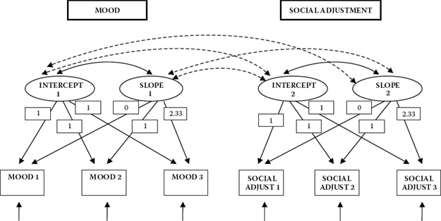
Figure 11.1. Hypothesized latent growth curve model.

The numerical values assigned to the paths flowing from the Intercept and Slope factors to the observed variables represent fixed parameters in the model. The 1’s specified for the paths flowing from each Intercept factor to each of its related outcome variables indicate that each is constrained to a value of 1.0. This constraint reflects the fact that the intercept value remains constant across time for each individual (Duncan et al., 2006). The values of 0, 1, and 2.33 assigned to the Slope regression paths represent Times 1, 2, and 3, respectively. These constraints address the issue of model identification; they also ensure that these factors can be interpreted as slopes. Three important points are of interest with respect to these fixed slope values. First, technically speaking, the first path (assigned a zero value) is really nonexistent and, therefore, has no effect. Although it would be less confusing to simply eliminate this parameter, it has become customary to include this path in the model, albeit with an assigned value of zero (Bentler, 2005). Second, these values represent the time intervals of 1, 4, and 8 months following surgery, albeit adjusted to take into account that, for our purposes here, Time 1 actually begins 1 month following the true initial testing point of 1 week following surgery. Unfortunately, due to the absence of scores for social adjustment at baseline (i.e., 1 week post surgery), only three of the four actual time points can be considered. As such, the values of 0, 1, and 2.33 represent a linear transformation of scores at Times 2, 3, and 4 (i.e., 1, 4, and 8 months post surgery) in order to establish initial status.² Finally, although the choice of fixed values assigned to the Slope factor loadings is arbitrary, it is important to realize that the Intercept factor is tied to a time scale (Duncan et al., 2006). Thus, any shift in fixed loading values on the Slope factor will necessarily modify the scale of time bearing on the Intercept factor, which, in turn, will influence interpretations related to the Intercept mean and variance. Relatedly, the variances and correlations among the factors in the model will change depending on the chosen coding (see, e.g., Biesanz, DeebSossa, Papadakis, Bollen, & Curran, 2004; Blozis & Cho, 2008).

In this section, our focus is on the modeling of intraindividual change. Within the framework of SEM, this focus is captured by the measurement model, the portion of a model that, as you well know at this point in the book, incorporates only linkages between the observed (i.e., outcome) variables and their underlying unobserved factors. As such, the only parts of the model in Figure 11.1 that are relevant to intraindividual change are (a) the regression paths linking the six outcome variables to the two Intercept and two Slope factors, (b) the factor variances and covariances, and (c) the related residuals associated with the outcome variables.

Essentially, we can think of this part of the model as an ordinary factor analysis model with two special features. First, all the loadings are fixed; that is, there are no unknown factor loadings. Second, the particular pattern of fixed loadings plus the mean structure allows us to interpret the factors as Intercept and Slope factors. As in all factor models, the present case argues that each woman's mood and social adjustment scores, at each of three time points (Time 1 = 0; Time 2 = 1; Time 3 = 2.33), are a function of three distinct components: (a) a factor loading matrix of constants (1; 1; 1) and known time values (0; 1; 2.33) that remain invariant across all individuals, multiplied by (b) an LGC vector containing individual-specific and unknown factors that in LGC models are called individual growth parameters (Intercept, Slope), plus (c) a vector of individual-specific and unknown errors of measurement (residuals of the outcome variables). Whereas the LGC vector represents the within-person true change in (self-perceived) mood and social adjustment over time, the residual or error vector represents the within-person noise that serves to erode these true change values (Willett & Sayer, 1994).

In preparing for transition from the modeling of intraindividual change to the modeling of interindividual change, it is important that we review briefly the basic concepts underlying the analyses of MACS in SEM (see also Chapter 8). When population means are of no interest in a model, analysis is based on only covariance structure (COVS) parameters. As such, all scores are considered to be deviations from their means, and, thus, the constant term (represented as α in a regression equation) equals zero. Given that mean values played no part in the specification of the Level 1 (or within-person) portion of our LGC model, the analysis of COVS was sufficient. However, in moving to Level 2, the between-person portion of the model, interest focuses on mean values associated with the Intercept and Slope growth factors; these values in turn influence the means of the outcome variables. Because both levels are involved in the modeling of interindividual differences in change, analyses are now based on MACS.

Modeling Interindividual Differences in Change

Level 2 argues that, over and above hypothesized linear change in mood and social adjustment over time, trajectories will necessarily vary across all Hong Kong women as a consequence of different intercepts and slopes. Within the framework of SEM, this portion of the model reflects that which we recognize as the structural model in that it typically represents relations among unobserved factors. However, in LGC models, structure is limited to only the means and variances of the Intercept and Slope growth factors. Whereas the means convey information regarding average intercept and slope values, the variances yield information related to individual differences in intercept and slope values. Specification of these parameters, then, makes possible the estimation of interindividual differences in change.

Let's now reexamine Figure 11.1 in more specific terms in order to clarify information bearing on possible differences in change across time. Within the context of only the first domain of mood, interest focuses on five parameters that are key to determining between-person differences in change: two means (Intercept1; Slope1), two variances (Intercept1; Slope1), and one covariance (between Intercept1 and Slope1). The means represent the average population values for the Intercept and Slope and answer the questions “What is the population initial level of mood at one month post surgery?” and “What is the population trajectory of true change in mood across 8 months post surgery?” The variances represent deviations of the individual Intercepts and Slopes from their population means, thereby reflecting population interindividual differences in the initial (1 month post surgery) mood self-rating scores and the rate of change in these scores, respectively. Addressing the issue of variability, these key parameters answer the question “Are there interindividual differences in the starting point and growth trajectories of mood in the population?” Finally, the Intercept-Slope covariance represents the population covariance between any deviations in initial status and rate of change and answers the question “Is there any evidence of interindividual differences in the association between initial status and rate of change in mood across an 8-month time span?”

Now that you have a basic understanding of LGC modeling in general and as it bears specifically on the hypothesized dual domain model shown in Figure 11.1, let's turn next to the Mplus input file and testing of this model.

Mplus Input File Specification and Output File Results

Testing for Validity of the Hypothesized Model

Input File 1

Displayed in Figure 11.2, you will see two input files related to this initial testing of the model. Whereas the one on the top left represents the short and preferred LGC specification, the one on the bottom right (labeled in the TITLE as Alternative Specification) specifies the model in a logical step-by-step manner that is relatively straightforward and perhaps easier to follow. Regardless of which form of specification is used, both input files generate the same output file. Turning first to the VARIABLE command, you will see that the data comprise 11 variables, only 6 of which will be used in this initial analysis (MOOD2, MOOD3, MOOD4, SOCADJ2, SOCADJ3, and SOCADJ4).³ Second, as noted in this chapter, due to a relatively minor degree of attrition, there are missing scores in the data. We alert the program to these missing values through use of the MISSING option, which in these data can be identified by the presence of an asterisk (*). This identification process is applied to all variables in the data.

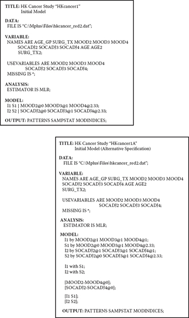
Figure 11.2. Mplus input files for model 1 shown in short (on the left) and long forms.

As discussed in Chapter 8, when continuous variable data are missing, whether they are missing completely at random (MCAR) or missing at random (MAR), Mplus is capable of taking such missingness into account through specification of the MLR estimator for which the standard errors are robust. Thus, under the ANALYSIS command, you will see that the ESTIMATOR option has been invoked and use of MLR estimation specified.

Thus far, our review of specifications in the two input files comprising Figure 11.2 has revealed them to be identical. However, in moving on to the MODEL command, they become substantially different. Because I believe you may find the alternative specification on the bottom right to be the easier of the two to follow, let's turn our attention to this input file first, accompanied by the portrayal of the model itself in Figure 11.1. The first four lines of specifications are pertinent to the regression paths flowing from the Intercept and Slope associated with each of the two domains of interest, mood and social adjustment. The first line specifies that the intercept for mood (I1) is measured by MOOD2, MOOD3, and MOOD4 (albeit labelled as MOOD1, MOOD2, and MOOD3 in Figure 11.1 for purpose of the introductory model; see Note 3). Likewise, the second line specifies that MOOD2 through MOOD4 also measure the slope for MOOD (S1). In both cases, each of the regression paths is specified as a fixed parameter in the model. Whereas the regression paths associated with I1 are constrained to a value of 1.00 (MOOD2@1 – MOOD3@1), those associated with S1 are constrained to values of 0.00, 1.00, and 2.33 for MOOD2 through MOOD4, respectively. The next two lines, of course, follow the same pattern for the second domain of social adjustment.

The two WITH statements in Lines 5 and 6 under the MODEL command specify that the Intercept and Slope factors covary for both the mood and social adjustment domains. Because this covariance is assumed in LGC modeling, as noted, it is default in Mplus.

The parenthesized information appearing in Lines 7 and 8 merely serves to group the variables according to their function as outcome variables in the model. As indicated, each of these six outcome variables is fixed at a value of zero. This specification relates to the intercepts of these variables, which are fixed at zero by default.

The final two parenthesized statements indicate that the Intercept and Slope for mood S1]) serve as a set of parameters in the model; likewise the Intercept and Slope factors for social adjustment ([I2 S2]).

Now that we have dissected the longer specification of our dual domain LGC model, let's turn back to the input file on the upper left-hand side of Figure 11.2 and focus on the much abbreviated MODEL command. Here we find only two statements—one pertinent to mood, and the other to social adjustment. These two statements represent exactly the same model specifications as the longer form in the alternative input file. This more concise specification is made possible through implementation of several related Mplus defaults. With respect to the dual domain LGC model hypothesized and tested in this chapter, these defaults are as follows: (a) The coefficients of each intercept factor are fixed at 1.00, (b) the intercepts of the outcome variables are fixed to zero, (c) the means and variances of both the Intercept and Slope factors are estimated, (d) the factor covariance between each Intercept-Slope pair is estimated, (e) cross-domain factor covariances are estimated, (f) residual variances of the outcome variables are estimated and allowed to vary across time points, and (g) residual covariances are assumed to be zero.

The | symbol is used to name and define the Intercept and Slope factors comprising the LGC model. Appearing on the left side of the | symbol are the names of the Intercept and Slope factors pertinent to each domain of interest. Thus, in the present case, we see I1 S1 specific to mood, and I2 S2 specific to social adjustment. Appearing on the right side of the | symbol are the outcome variable names together with time scores for the LGC model. As with the longer version of this input file, time scores for the Slopes are fixed at 0, 1, and 2.33 and, as such, make it possible to define a linear growth model with nonequidistant time points.

Finally, because the data used for this application have missing values, the option of PATTERNS has been requested, along with SAMPSTATS and MODINDICES. As we observed in Chapter 8, this option provides us with an informed picture of the configuration and extent to which the data are incomplete.

Output File 1

Having reviewed the two alternative input files for our LGC model, let's turn next to Table 11.1, where a summary of the missing data results in the output file is presented. Identified first in the output is the number of missing data patterns, which is shown to be 15. This summary information is followed by a detailed breakdown of these 15 patterns, together with the score frequency for each pattern. Given that an x represents no missing data, we can see that Pattern 1, for example, represents the case for complete data and has a frequency of 307 scores. Given a total sample of 405 cases, we now know that there are 98 women for whom there are missing scores and that these missing scores are represented by 14 different patterns. A review of the pattern frequencies helps to fill in the blanks on this information. For example, whereas Pattern 9 reveals that 23 women had complete scores for only MOOD2 and SOCADJ2, Pattern 15 reveals that it has complete data for only one of the six variables (SOCADJ3); each of the remaining variables has missing data. The final piece of information for this section of the output file reports on the proportion of data present. As can be seen in the table, the largest proportion of data is provided at Time 1 with 95.9% scores present for MOOD2 and 96.4% for SOCADJ2.

Table 11.1 Mplus Output for Model 1: Missing Data Statistics

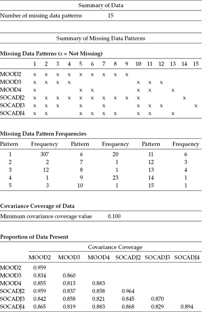
Table 11.2 Mplus Output for Model 1: Sample Statistics

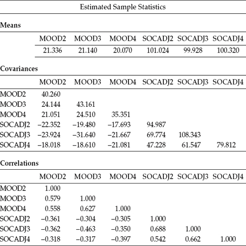
Presented next, in Table 11.2, are the estimated sample statistics for these data. Turning first to the means of the outcome variables, we can see that there is minimal fluctuation across the 8 months for both mood and social adjustment. In fact, there appears to be virtually no difference in the mood scores between those collected at 1 month post surgery and those collected after 4 months; scores at Time 3 (i.e., after 8 months post surgery) were slightly lower. Social adjustment also showed little change over the 8-month period, albeit the lowest score here occurred at the second time point (4 months post surgery). These mean scores suggest that evidence of change in the slopes related to both constructs across an 8-month postsur-gery period will likely be minimal.

Appearing next in Table 11.2 is the covariance matrix. In reviewing the variances on the main diagonal of this matrix, we can see that for both mood and social adjustment, scores collected 4 months post surgery exhibited the most variability across the women, dropping off substantially at 8 months post surgery. That a wide fluctuation of individual trajectories occurred at time point 2 (4 months post surgery) seems to suggest that it is at the midpoint of the healing process when the perceptions of the women varied widely in terms of both their emotional well-being and their ability to cope with the situation socially. Appearing last in Table 11.2 is the correlation matrix, where we can observe the strongest association to be between SOCADJ2 and SOCADJ3, the intersection between perceptions of social adjustment at Time 1 and Time 2.

Before turning to SEM results related to the testing of the hypothesized model, I wish to show you an example of the PLOT command provided by Mplus as it works easily and well in enabling you to have a more detailed look at your data. Details related to this facility were outlined in Chapter 2. Graphical presentations resulting from the PLOT command can be inspected following completion of the analyses using a dialog based postprocessing graphics module. These graphical presentations are tagged as .gph files and are accessed in the same way as both the model input and output files. The input file related to specification of the PLOT command is presented in Figure 11.3, and the process of accessing the graph file shown in Figure 11.4.

Once you access a graph file, you are offered the choice of viewing variables within the context of a histogram or scatterplot (sample values), or as observed individual values; you can also select the number of cases to be included in the graph, as well as whether they should be selected consecutively or randomly. Presented in Figures 11.5, 11.6, and 11.7 are three different views of individual values pertinent to the first 15 women in our breast cancer database. Turning first to Figure 11.5, note first (on the bar under the toolbar) the term Process 1. Accordingly, this first graph limits the trajectories to only the first domain of mood. However, right clicking on any of the points will provide you with extended information related to scores for any particular case. As illustrated in Figure 11.5, right clicking on the highest score for Time 1 revealed this trajectory to belong to Individual 3, along with the other scores on both domains for this person. Figure 11.6 shows the trajectories for the same Individual 3, albeit specific to Domain 2, social adjustment. Note that the bar at the top of this set is labeled Process 2. Again, right-clicking on the initial score of 80.667 listed all scores for this individual. Finally, Figure 11.7 shows you how to access further information, which in this case is how to move to another set of 15 individuals. Because I opted for consecutive selection, this next sample would comprise scores for Individuals 16 through 30.

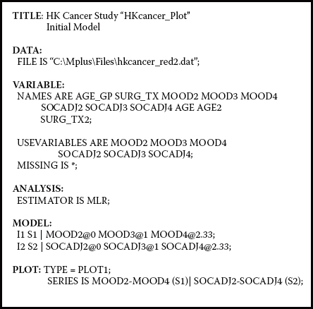
Figure 11.3. Mplus input file showing the PLOT command.

Figure 11.4. Mplus dropdown menu for retrieval of graphical output.

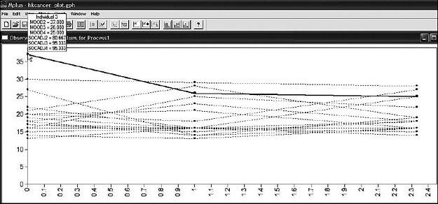
Figure 11.5. Mplus graphical output: Individual plot showing scores for first 15 subjects over three time points for mood.

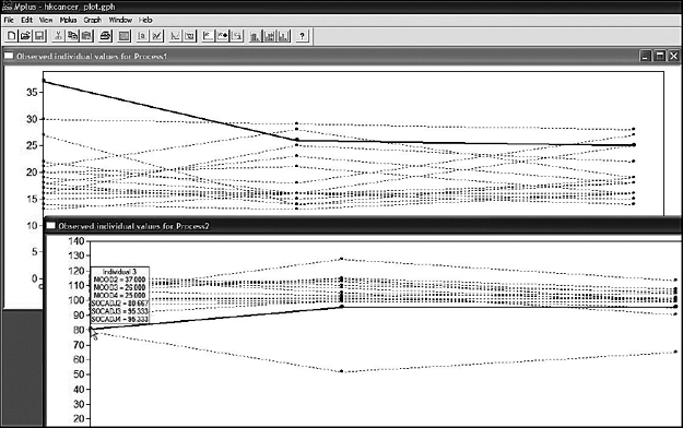
Figure 11.6. Mplus graphical output: Individual plot showing in the foreground scores for first 15 subjects over three time points for social adjustment.

Figure 11.7. Mplus graphical output showing method for obtaining plot for an alternative set of scores.

Table 11.3 Mplus Output for Model 1: Selected Goodness-of-Fit Statistics

Tests of Model Fit
Chi-Square Test of Model Fit
Value	36.036*
Degrees of freedom	7
p-value	0.0000
Scaling Correction Factor for MLR	1.118
CFI/TLI
CFI	0.944
TLI	0.879
Root Mean Square Error of Approximation (RMSEA)
Estimate	0.104
90 percent confidence interval (CI)	0.072	0.138
Probability RMSEA <= .05	0.004
Standardized Root Mean Square Residual (SRMR)
Value	0.086

* The chi-square value for MLM, MLMV, MLR, ULSMV, WLSM, and WLSMV cannot be used for chi-square difference tests. MLM, MLR, and WLSM chi-square difference testing is described in the Mplus “Technical Appendices” at http://www.statmodel.com. See chi-square difference testing in the index of the Mplus User's Guide (Muthén & Muthén, 2007-2010).

At this point, I think we're ready to move on to examining results from our test of the hypothesized model. Presented in Table 11.3 are the key goodness-of-fit statistics. Recall that due to the presence of incomplete data, we selected the MLR estimator as it can correct the maximum likelihood (ML) chi-square (χ²) statistic to take this missingness into account. Here we find a corrected χ² value of 36.036 with seven degrees of freedom; the scaling correction factor is reported to be 1.118. Consistent with notation of this caveat elsewhere in the book, the * accompanying the χ² statistic serves as a reminder that calculation of χ² difference tests based on (in this case) the MLR estimator between any two competing models is inappropriate.

Before reviewing the remaining fit statistics, however, I think it's important that you clearly understand the source of the seven degrees of freedom. First, let's think about the number of pieces of information with which we have to work here. With LGC models, we are dealing with both the means as well as the covariances of the outcome variables. Thus, given six outcome variables, the number of covariances will be 6 (6 + 1)/2, which equals 21; taking into consideration the six observed means, we have a total of 27 pieces of information upon which the analyses will be based. Consider now the number of freely estimated parameters in the model (see Figure 11.1); these are as follows:

• Four factor means S1, I2, and S2)

• Four factor variances S1, I2, and S2)

• Six residual variances (MOOD2, MOOD3, MOOD4, SOCADJ2, SOCADJ3, and SOCADJ4)

• Two factor covariances (I1 with S1; and I2 with S2)

• Four cross-domain factor covariances (I1 with I2; I1 with S2; S1 with S2; and S1 with I2)

Accordingly, given 27 pieces of information and 20 estimated parameters, the number of degrees of freedom should be seven, which indeed it is.

Moving on to the remainder of Table 11.3, we find values of 0.944 and 0.879 for the CFI and TLI, respectively. Although the CFI value is moderately good, the TLI value is clearly unacceptable. Likewise, the Root Mean Square Error of Approximation (RMSEA) value of 0.104 and Standardized Root Mean Square Residual (SRMR) value of 0.086 are also less than acceptable. Thus, it is clear that some modification to the model is needed.

Shown in Table 11.4 is the listing of only one modification index suggesting that specification of a covariance between the residual variances associated with SOCADJ3 and MOOD3 would lead to a substantially better fit to the hypothesized model. Indeed, the expected parameter change (EPC) value of -9.657 suggests a fairly strong relation between these two outcome variables. Given that mood was measured by the 12-item Chinese Health Questionnaire (Cheng & Williams, 1986), which taps into symptoms of anxiety and depression, low scores are indicative of a more positive mood; the resulting negative EPC value therefore is reasonable. Given both the estimated size of this covariance parameter, together with its substantive plausibility, the hypothesized model was respecified and reestimated accordingly.

Table 11.4 Mplus Output for Model 1: Modification Indices (MIs)

Model Modification Indices
	MI	Expected Parameter Change (EPC)	Standard EPC	StdYX EPC
WITH Statements SOCADJ3 WITH MOOD3	26.452	-9.637	-9.637	-0.361

Table 11.5 Mplus Output for Model 2: Selected Goodness-of-Fit Statistics

Tests of Model Fit
Chi-Square Test of Model Fit
Value	6.590
Degrees of freedom	6
p-value	0.3605
Scaling Correction Factor for MLR	1.085
CFI/TLI
CFI	0.999
TLI	0.997
Root Mean Square Error of Approximation (RMSEA)
Estimate	0.016
90 percent confidence interval (CI)	0.000	0.069
Probability RMSEA <= .05	0.806
Standardized Root Mean Square Residual (SRMR)
Value	0.042

Testing for Validity of Model 2

Let's now review goodness-of-fit statistics related to this modified model, which are reported in Table 11.5. Clearly, the addition to Model 1 of the residual covariance between MOOD3 and SOCADJ3 resulted in a highly improved fit to the data, as evidenced from the CFI = 0.999, TLI = 0.997, RMSEA = .016, and SRMR = 0.042. Now that we have an extremely well-fitting model, let's review parameter estimates as a check for any that may be nonsignificant, thereby allowing us to obtain a more parsimonious model through their deletion; this search is limited to only modeled covariances, as all other parameters must remain intact. These estimated values are presented in Table 11.6.

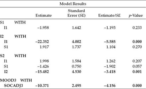
In reviewing these estimates in Table 11.6, you will readily note that all statistically significant covariance estimates have been highlighted in bold. Accordingly, in addition to the residual covariance added in Model 2, there are only two other covariance estimates that are statistically significant: (a) the originally hypothesized association between the intercept and slope for social adjustment (S2, I2), and (b) an association between the intercepts for social adjustment and mood (I2, Given the substantive rationality of this latter covariance, it is reasonable to retain this parameter in the model. Thus, in the interest of parsimony, a final LGC model was specified in which the following covariances were deleted: (a) the slope and intercept for mood (S1, I1), (b) the slope for mood and the intercept for social adjustment (S1, I2), (c) the slope for social adjustment and the intercept for mood (S2, I1), and (d) the slopes for social adjustment and mood (S2, S1).

Table 11.6 Mplus Output for Model 2: Selected Parameter Estimates

Testing for Validity of the Final Model

Output File 2

Turning first to the goodness-of-fit statistics for this final model (see Table 11.7), we note that, except for the MLR chi-square value, which now has 10, rather than 6 degrees of freedom (due to deletion of the four covariance parameters), the remaining CFI, TLI, RMSEA, and SRMR results remained close to the former values for Model 2. As such, we can feel confident that interpretations of the final growth results are based on an extremely well-fitting model.

Let's now examine the resulting parameter estimates, which are reported in Table 11.8. Presented first are the factor covariance estimates, which of course are all significant. Turning first to the between-domain covariance of I2 with I1, we find the negative value of -19.870. This result suggests that for women whose scores for mood were high at Time 1 (1 month following surgery), their scores for social adjustment were low. Given my earlier explanation regarding the assessment scale used in measuring mood, this inverse relation between the two domains is both logical and reasonable.

Table 11.7 Mplus Output for Final Model: Selected Goodness-of-Fit Statistics

Tests of Model Fit
Chi-Square Test of Model Fit
Value	13.530
Degrees of freedom	10
p-value	0.1955
Scaling Correction Factor for MLR	1.247
CFI/TLI
CFI	0.993
TLI	0.990
Root Mean Square Error of Approximation (RMSEA)
Estimate	0.030
90 percent confidence interval (CI)	0.000	0.067
Probability RMSEA <= .05	0.778
Standardized Root Mean Square Residual (SRMR)
Value	0.040

The second reported covariance represents the within-domain link between scores on social adjustment at Time 1 and at Time 3 (i.e., 8 months later). That these scores are also negative is rather interesting as they suggest that for women who perceived their future social interaction among friends and family in a rather pessimistic light at 1 month following breast cancer surgery, the reverse situation occurred; that is, these perceptions became more optimistic over the 8-month postsurgery period. Likewise, the reverse perceptions were realized.

The third covariance reported relates to the subsequently specified residual covariance between mood and social adjustment at Time 2, which is shown to be statistically significant.

The next two categories of results reported in Table 11.8 (Means and Variances) are typically of most importance in LGC modeling. All statistically significant estimates have been highlighted in bold. We turn first to results for the Intercept and Slope means. These estimates convey information related to both the average scores on mood and social adjustment at Time 1 and the average rate of change in these scores across the 8-month period. As shown in Table 11.8, only the estimated slope for social adjustment was found to be nonsignificant. Let's look first at the results for mood. These estimates indicate that, although the average self-reported score at 1 month post surgery was 21.397 (the Intercept), this score decreased, on average, by 0.550 (the Slope) over the subsequent 8 months. This finding implies that as time following surgery increases, women tend gradually to report a more positive mood. With respect to social adjustment, we note that, on average, the score at 1 month following surgery was 100.926, albeit with negligible change over the next 8 months.

Table 11.8 Mplus Output for Final Model: Selected Parameter Estimates

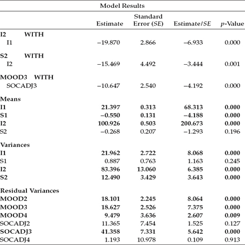
Turning next to the variances, we see that again we have one statistically nonsignificant estimate (S1), the Slope for mood. As noted earlier, these parameters represent deviation from the average intercept and slope in the population and, as such, yield information on interindividual differences both in the initial status of mood and social adjustment and in their change over time from 1 month to 8 months post surgery. Such evidence provides strong justification for the incorporation of predictor variables in subsequent analyses in an effort to explain this variation. We address this issue following this review of the parameter estimates.

Finally, the last six entries in Table 11.8 provide estimates of the residual variance associated with each occasion of measurement for mood and social adjustment. Although these error terms were statistically significant with respect to mood at each of the three time points, they were only so for Time 2 (4 months post surgery) for social adjustment.

Hypothesized Covariate Model: Age and Surgery as Predictors of Change

As noted earlier in the chapter, provided with evidence of interindividual differences, we can then ask whether, and to what extent, one or more predictors might explain this heterogeneity. For our purposes here, we ask whether statistically significant heterogeneity in the individual growth trajectories (i.e., intercept and slope) of mood and social adjustment can be explained by age and/or type of surgery performed. As such, two questions that we might ask are “Do self-perceptions of mood and social adjustment following breast cancer surgery differ for Hong Kong women according to their age (0 = < 51 years; 1 = > 50 years) and/or type of surgical treatment (0 = lumpectomy; 1 = mastectomy)⁴ at Time 1 (1 month following surgery)?” and “Does the rate at which self-perceived mood and social adjustment change over time differ according to age and/or type of surgery?” To answer these questions, the predictor variables of age and surgery were incorporated into the model. This covariate model represents an extension of our final best fitting model and is shown schematically in Figure 11.8.

In reviewing this path diagram, I draw your attention to the addition of three new components: (a) the four regression paths leading from each of the predictor variables (age and surgery) to the Intercept and Slope factors associated with mood and social adjustment, (b) the double-headed arrow representing the covariance between I1 and I2, and (c) the double-headed arrow representing the covariance between the residual variances for MOOD3 and SOCADJ3. Note also that, given findings of a nonsignificant estimate for the postulated covariance between the intercept and slope for mood in the initially hypothesized model, this parameter does not appear in this covariate model. Of primary interest here are the regression paths that flow from the predictor variables to I1, S1, I2, and S2 for the two domains of mood and social adjustment as they hold the key in answering the question of whether the trajectories of mood and social adjustment differ across age and surgery. Also worthy of note is the fact that, with the addition of the two predictor variables to the model, interpretation of the Intercept and Slope residual variances necessarily changes. Whereas these parameters in the previous model (in which no predictors were specified) represented deviations between the Intercept and Slope factors, and their population means, within the framework of the current model they now represent variation remaining in the intercepts and slopes after all variability in their prediction by age and surgery has been explained. That is, they represent the adjusted values of the factor intercepts and slopes after partialing out the linear effect of the predictors of change (Willett & Keiley, 2000).

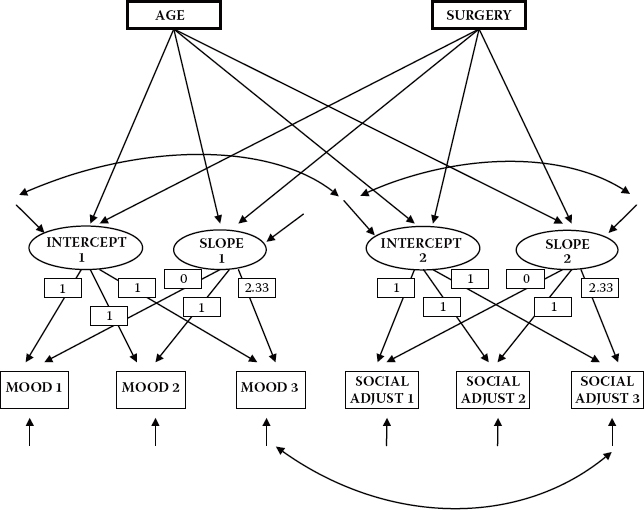
Figure 11.8. Hypothesized covariate model showing age and surgery as predictor variables.

Input File

Before examining the results of analyses stemming from the test of this covariate model, let's first review the related input Mplus file presented in Figure 11.9. Three specifications are of prime interest here. First, note under the VARIABLE command that the USEVARIABLES option now includes the variables AGE2 and SURG_TX2, the two predictor variables. Of import here is that although these two variables are categorical, there is no need to specify this information as they operate as only independent variables in the model. Second, recall that in our testing of the initially hypothesized model, we found four factor covariance parameters to be nonsignificant, and in the interest of parsimony they were subsequently deleted; in Mplus, this deletion is accomplished by fixing the related parameters to zero. Accordingly, the four WITH statements representing these nonsignificant covariance parameters appear in lines 4 through 7 under the MODEL command. Finally, the last two lines of model input represent specifications related to the two predictor regression paths. As such, the Intercept and Slope factors for both mood and social adjustment are shown to load on predictor variables labeled in the data set as AGE2 and SURG_TX2.

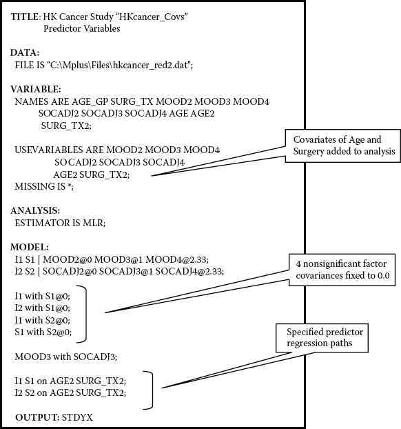
Figure 11.9. Mplus input file for covariate model.

Table 11.9 Mplus Output for Covariate Model: Selected Goodness-of-Fit Statistics

Tests of Model Fit
Chi-Square Test of Model Fit
Value	16.622
Degrees of freedom	14
p-value	0.2769
Scaling Correction Factor for MLR	1.147
CFI/TLI
CFI	0.996
TLI	0.992
Root Mean Square Error of Approximation (RMSEA)
Estimate	0.022
90 percent confidence interval (CI)	0.000	0.055
Probability RMSEA <= .05	0.911
Standardized Root Mean Square Residual (SRMR)
Value	0.033

Output File

We turn now to the results for this covariance model and look first at the goodness-of fit statistics, which are presented in Table 11.9. Here again, we find an exceptionally good fit to the data (MLR χ²_[14] = 16.622; CFI = 0.996; TLI = 0.992; RMSEA = 0.022; SRMR = 0.033). In the interest of space restrictions and because the parameters of primary interest with this model are the factor regression paths of individual change on the predictor variables of age and surgery, only findings related to these parameters are presented in Table 11.10.

Turning first to results for mood, we find that whereas age was a statistically significant predictor of initial status (I1 on AGE2; -1.637, estimate/ standard error [SE] = -2.647), it was not so for rate of change (S1 on AGE2; -0.207, estimate/SE = -0.795). Given a coding of 0 for women < 51 years and 1 for women > 50 years, these findings suggest that reported mood scores, on average, were lower at Time 1 (by 1.637 units) for women over the age of 50 than they were for younger women. The nonsignificant findings related to the slope suggest that any differences in the rate of change in these scores across the 8-month period between the two age groups were negligible. Likewise, type of SURGERY appeared to have no effect on either the initial status of mood (I1 ON SURG_TX2; -0.027, estimate/SE = -0.036) or its rate of change across time (S1 on SURG_TX2; -0.339, estimate/SE = -1.006).

Table 11.10 Mplus Output for Covariate Model: Selected Parameter Estimates

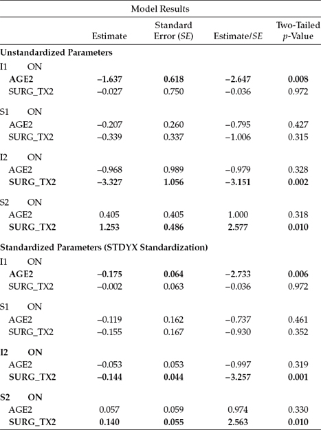
In contrast, results related to social adjustment revealed type of SURGERY to be a significant predictor of both initial status (I2 on SURG_TX2; -3.327, estimate/SE = -3.151) and its rate of change across the 8-month period (S2 on SURG_TX2; 1.253, estimate/SE = 2.577). Based on the coding system of 0 for women who underwent lumpectomy and 1 for those who underwent mastectomy, these findings suggest that whereas women who underwent a mastectomy had lower scores on social adjustment at initial status than women who underwent a lumpectomy (by -3.327), their rate of change in this perception over the 8-month period was somewhat faster (by 1.253). Thus, although initially social adjustment among women having a lumpectomy was better than it was among women having a mastectomy, over time this advantage diminished. Finally, age was found not to be a significant predictor of either initial status (I2 on AGE2; -0.968, estimate/SE = -0.979) or rate of change (S2 on AGE2; 0.405, estimate/SE = 1.000) for social adjustment.

In closing out this chapter, I draw from the work of Willett and Sayer (1994, 1996) in highlighting several important features captured by the LGC modeling approach in the investigation of change. First, the methodology can accommodate anywhere from 3 to 30 waves of longitudinal data equally well. Willett (1988, 1989) has shown, however, that the more waves of data collected, the more precise will be the estimated growth trajectory and the higher will be the reliability for the measurement of change. Second, there is no requirement that the time lag between each wave of assessments be equivalent. Indeed, LGC modeling can easily accommodate irregularly spaced measurements, but with the caveat that all subjects are measured on the same set of occasions. Third, individual change can be represented by either a linear or a nonlinear growth trajectory. Although linear growth is typically assumed by default, this assumption is easily tested and the model respecified to address curvilinearity if need be. Fourth, in contrast to traditional methods used in measuring change, LGC models allow not only for the estimation of measurement residual (i.e., error) variances, but also for their autocorrelation and fluctuation across time in the event that tests for the assumptions of independence and homoscedasticity are found to be untenable. Fifth, multiple predictors of change can be included in the LGC model. They may be time invariant, as in the case of gender, and as applied in the present chapter, or they may be time varying (see, e.g., Curran, Muthén, & Harford, 1998; Willett & Keiley, 2000). Finally, the three key statistical assumptions associated with LGC modeling (linearity, independence of measurement error variances, and homoscedasticity of measurement error variances), although not demonstrated in this chapter, can be easily tested via a comparison of nested models (see Duncan et al., 2006).

Notes

1.	In the original study, this construct was termed psychological morbidity.
2.	Had all time points been used, these values would have been 0, 1, 2, and 3.
3.	Recall that, for our purposes here, analyses are based on scores from the second through fourth time points, as noted in this chapter (albeit we have considered them to represent Times 1 through 3 for convenience here), hence the numbered labels 2 through 4.
4.	The two categories of age were formulated on the basis of average physiological age of menopause, thereby yielding a premenopausal group (< 51 years, coded as 0) and a postmenopausal group (> 50 years, coded as 1). The two categories of surgery type comprised women whose breast cancer involved a lumpectomy (coded as 0) and those for whom surgery involved a mastectomy (coded as 1).