CHAPTER 11

Spectral Allocation—Impact on Network Hardware Design

In Parts I and II of the book we covered handset hardware and handset software form factor. We said handset hardware and software has a direct impact on offered traffic, which in turn has an impact on network topology. The SIM/USIM in the subscriber's handset describes a user's right of access to delivery and memory bandwidth, for example, priority over other users. Handset hardware dictates image and audio bandwidth and data rate on the uplink (CMOS imaging, audio encoding). Similarly, handset hardware dictates image and audio bandwidth and data rate on the downlink (speaker/headset quality and display/display driver bandwidth).

In this part of the book we discuss how network hardware has to adapt. We have defined that there is a need to deliver additional bandwidth (bandwidth quantity), but we also have to deliver bandwidth quality. We have defined bandwidth quality as the ability to preserve product value—the product being the rich media components captured from the subscriber (uplink value).

Searching for Quality Metrics in an Asynchronous Universe

Delay and delay variability and packet loss are important quality metrics, particularly if we need to deliver consistent end-to-end application performance. The change in handset hardware and software has increased application bandwidth—the need to simultaneously encode multiple per-user traffic streams, any one of which can be highly variable in terms of data rate and might have particular quality of service requirements. This chapter demonstrates how offered traffic is becoming increasingly asynchronous—bandwidth is becoming burstier—and how this exercises network hardware.

In earlier chapters we described how multiple OVSF codes created large dynamic range variability (peak-to-average ratios) that can put our RF PAs into compression. This is a symptom of bursty bandwidth. On the receive side of a handset or Node B receiver, front ends and ADCs can be put into compression by bursty bandwidth (and can go nonlinear and produce spurious products in just the same way as an RF PA on the transmit path). As we move into the network, similar symptoms can be seen. Highly asynchronous bursty bandwidth can easily overload routers and cause buffer overflow. Buffer overflow causes packet loss. Packet loss in a TCP protocol-based packet stream triggers “send again” requests, which increase delay and delay variability and decrease network bandwidth efficiency.

We need to consider in detail the impact of this increasingly asynchronous traffic on network architectures and network hardware. In practice, we will see that neither traditional circuit-switched-based architectures nor present IP network architectures are particularly well suited to handling highly asynchronous traffic. We end up needing a halfway house—a circuit-switched core with ATM cell switching in the access network, both optimized to carry IP-addressed packet traffic.

In the first chapter of this Part, we study the RF parts of the network and how the RF subsystems need to be provisioned to accommodate bursty bandwidth. We will find that adding a radio physical layer to a network implicitly increases delay and delay variability. It is therefore particularly important to integrate radio layer and network layer performance in order to deliver a consistent end-to-end user experience.

Typical 3G Network Architecture

Figure 11.1 shows the major components in a 3G network, often described as an IP QoS network—an IP network capable of delivering differentiated quality of service. To achieve this objective, the IP QoS network needs to integrate radio physical layer performance and network layer performance. The IP QoS network consists of the Internet Protocol Radio Access Network (IPRAN) and the IP core replacing the legacy Mobile Radio Switch Center (MSC).

The function of the Node B, which has replaced the base station controller (BTS), is to demodulate however many users it can see, in RF terms, including demodulating multiple per-user traffic streams. Any one of these channel streams can be variable bit rate and have particular, unique QoS requirements. Node Bs have to decide how much traffic they can manage on the uplink, and this is done on the basis of interference measurements—effectively the noise floor of the composite uplink radio channel. A similar decision has to be made as to how downlink RF bandwidth is allocated. The Node B also must arbitrate between users, some of whom may have priority access status. We refer to this process as IPRAN interference-based admission control.

Figure 11.1 IP QoS network.

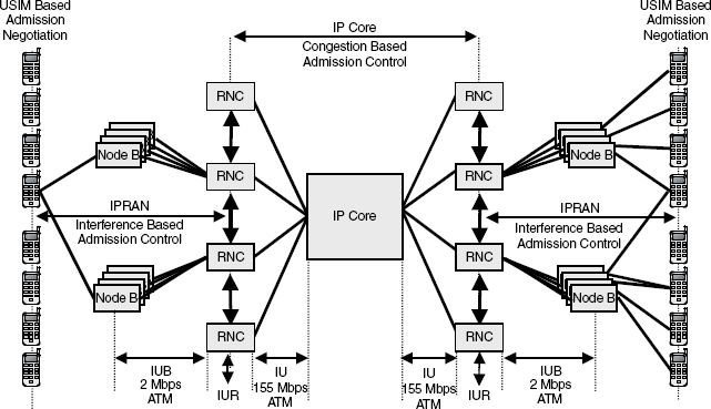
The RNCs job is to consolidate traffic coming from the Node Bs under its control. The RNC also has to load balance—that is, move traffic away from overloaded Node Bs onto more lightly loaded Node Bs and to manage soft handover—a condition in which more than one Node B is serving an individual user on the radio physical layer. The fourth handset down on the right-hand side of Figure 11.1, for example, is in soft handover between two Node Bs supported by two different RNCs. The handset is, more or less, halfway between two Node Bs. To improve uplink and downlink signal level, the RNC has decided that the handset will be served by two downlinks, one from each Node B. Both nodes will also be receiving an uplink from the handset. Effectively this means there will be two long codes on the downlink and two long codes on the uplink. The two uplinks will be combined together by the serving RNC, but this will require the serving RNC to talk to the other serving RNC (called the drift RNC). The same process takes place on the downlink.

The RNC has to make a large number of very fast decisions (we revisit RNC software in Chapter 17 in our section on network software), and the RNC-to-RNC communication has to be robust and well managed. The RNCs then have to consolidate traffic and move the traffic into the IP core. Admission control at this point is done on the basis of congestion measurements:

• Is transmission bandwidth available?
• If no transmission bandwidth is available, is there any buffer bandwidth available?

If no transmission bandwidth is available and no buffer bandwidth is available then packet loss will occur unless you have predicted the problem and choked back the source of the traffic.

RNC traffic management and inter-RNC communication is probably the most complex part of the IPRAN and is the basis for substantial vendor-specific network performance optimization. This is complex deterministic software executing complex decisions within tightly defined timescales. As with handset design, there is considerable scope for hardware coprocessors and parallel hardware multitasking in the RNC. As with handset design, we will show that network performance is also dependent on the RF performance available from the Node B—the Node B's ability to collect highly bursty traffic from users and deliver highly bursty traffic to users.

The Impact of the Radio Layer on Network Bandwidth Provisioning

Table 11.1 shows how the aggregated bit rate increases as we move into the network. The highly asynchronous traffic loading is supported on a 2 Mbps ATM bearer between the Node B and RNC and a 155 Mbps ATM bearer, or multiple bearers, between the RNC and IP core. The job of the IP core is to process traffic, and (we assume) a fair percentage of the traffic will be packetized. This is a packet-routed or, more accurately, packet-queued network.

The radio physical layer is delivering individual users at user bit rates varying between 15 kbps and 960 kbps. This is aggregated at the Node B onto multiple 2 Mbps ATM wireline transport (copper access), which is aggregated via the RNC onto multiple 155 Mbps ATM (copper). This is aggregated onto 2.5, 10, or 40 Gbps copper and optical fiber in the network core. The IP core may also need to manage highly asynchronous traffic from wireline ADSL/VDSL modems (offering bit rates from 56 kbps to 40 Mbps).

Table 11.1 Access Bandwidth/Network Bandwidth Bit Rates

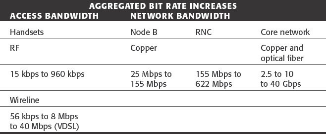
Table 11.2 Time Dependency versus Bit Rate

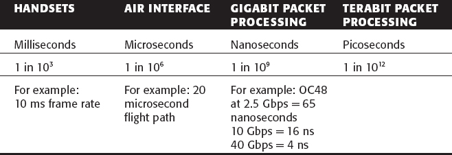
As throughput increases, processing speed—and processor bandwidth—increases (see Table 11.2). Routers must classify packets, and perform framing and traffic management. If we have added packet-level security, the router must perform a deep packet examination on the whole packet header to determine the security context.

The Circuit Switch is Dead—Long Live the Circuit Switch

We could, of course, argue that it is difficult to match the performance or cost efficiency of a circuit switch. Financially, many circuit switches are now fully amortized. They provide definitive end-to-end performance (typically 35 ms of end-to-end delay and virtually no delay variability) and 99.999 percent availability. Circuit switches achieve this grade of service by being overdimensioned, and this is the usual argument used to justify their imminent disposal. However, as we will see, if you want equivalent performance from an IP network, it also needs to be overdimensioned and ends up being no more cost effective than the circuit switch architecture it is replacing.

Circuit switches are also getting smaller and cheaper as hardware costs go down. Ericsson claims to be able to deliver a 60 percent size reduction every 18 months and a 30 percent reduction in power budget.

Consider the merits of a hardware switch. An AXE switch is really very simple in terms of software—a mere 20 million lines of code, equivalent to twenty 3G handsets! Windows 98 in comparison has 34 million lines of code. A hardware switch is deterministic. Traffic goes in one side of the switch and comes out the other side of the switch in a predictable manner. A packet-routed network, in comparison, might have lost the traffic, or misrouted or rerouted it, and will certainly have introduced delay and delay variability.

As session persistency increases (as it will as 3G handset software begins to influence user behavior), a session becomes more like a circuit-switched phone call. In a hardware-switched circuit-switched phone call, a call is set up, maintained, and cleared down (using SS7 signaling). In a next-generation IP network, a significant percentage of sessions will be set up, maintained, or cleared down (using SIP or equivalent Internet session management protocols).

A halfway house is to use ATM. This is effectively distributed circuit switching, optimized for bursty bandwidth.

Over the next few chapters we qualify IP QoS network performance, including the following factors:

• Its ability to meet present and future user performance expectations
• Its ability to deliver a consistent end-to-end user experience
• Its ability to provide the basis for quality-based rather than quantity-based billing

But let's begin by benchmarking base station and Node B performance.

BTS and Node B Form Factors

Node B is the term used within 3GPP1 to describe what we have always known as the base station. Node refers to the assumption that the base station will act as an IP node; B refers to base station. The Node B sits at the boundary between the radio physical layer (radio bandwidth) and the RNC, which in turn sits at the boundary between the IP radio access network (RAN) and the IP core network.

We have talked about the need for power budget efficiency in handset design and power budget efficiency in the switch. We also need power budget efficiency in the Node B so that we can get the physical form factor as small as possible. If we can keep power consumption low, we can avoid the need for fan cooling, which gives us more flexibility in where and how we install the Node B.

Typical design targets for a base station or Node B design would be to deliver a cost reduction of at least 25 percent per year per RF channel and a form factor reduction of at least 30 percent per year per channel.

Typical 2G Base Station Product Specifications

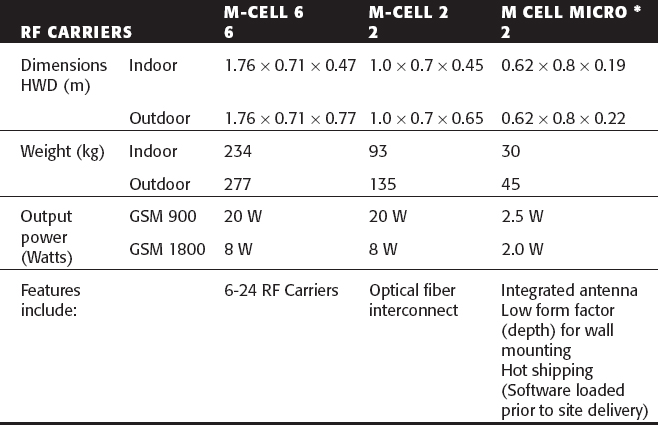
Table 11.3 gives some typical sizes and weights for presently installed GSM base stations supplied by Motorola. Although there are 195×200 kHz RF carriers available at 900 MHz and 375×200 kHz RF carriers available at 1800 MHz, it is unusual to find base stations with more than 24 RF carriers and typically 2 or 6 RF carrier base stations would be the norm. This is usually because 2 or 4 or 6 RF carriers subdivided by 8 to give 16, 32, or 48 channels usually provides adequate voice capacity for a small reasonably loaded cell or a large lightly loaded cell. Having a small number of RF carriers simplifies the RF plumbing in the base station—for example, combiners and isolators, the mechanics of keeping the RF signals apart from one another. Table 11.3 shows that hardware is preloaded with network software prior to shipment.

Table 11.3 Base Station Products: Motorola–GSM 900/1800/1900

Products from Nokia have a similar hardware form factor (see Table 11.4). This has the option of a remote RF head, putting the LNA (Low-Noise receive Amplifier) close to the antenna to avoid feeder losses. There is also the choice of weather protection (IP54/IP55; IP here stands for “intrinsic protection”).

Table 11.4 Base Station Products–Nokia–GSM 900/1800/1900

Table 11.5 Base Station Products–Ericsson–GSM 900/1800/1900

A Nokia PrimeSite product weighs 25 kg in a volume of 35 liters. This is a single RF carrier base station with two integrated antennas to provide uplink and downlink diversity.

Similar products are available from Ericsson, also including mast-mounted LNAs to improve uplink sensitivity. Table 11.5 gives key specifications, including number of RF carriers, and highlights additional features such as the inclusion of automatic hardware and software revision tracking.

The GSM specification stated that different vendor BTS products should be capable of working with different vendor BSCs. As you would expect, all BTSs have to be compatible with all handsets. Because GSM is a constant envelope modulation technique, it has been possible to deliver good power efficiency (typically >50 percent) from the BTS power amplifiers and hence reduce the hardware form factor. This has been harder to achieve with IS95 CDMA or IS136 TDMA base stations because of the need to provide more linearity (to support the QPSK modulation used in IS95 and the π/4DQPSK modulation used in IS136 TDMA).

Table 11.6 shows the specification for a Motorola base station capable of supporting AMPS, CDMA, and TDMA. The CDMA modem provides 1.25 MHz of RF channel bandwidth (equivalent to a GSM 6 RF carrier base station) for each RF transceiver with a total of 16 transceivers able to be placed in one very large cabinet to access 20 MHz of RF bandwidth—the big-is-beautiful principle. The linear power amplifier weighs 400 kg! The products are differentiated by their capacity—their ability to support high-density, medium-density, or very localized user populations (microcells).

Table 11.6 Base Station Products–Motorola–AMPS/N-AMPS/CDMA/IS136 TDMA

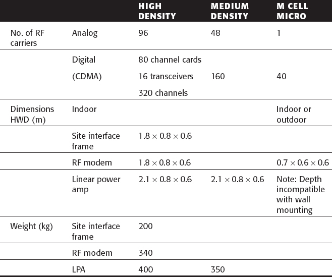
Table 11.7 shows a parallel product range from Ericsson for AMPS/IS136. These are typically 10 W or 30 W base stations (though a 1.5 W base station is available for the indoor microcell). The size is measured in terms of number of voice paths per square meter of floor space. Again, the product range is specified in terms of its capacity capabilities (ability to support densely populated or less densely populated areas).

Table 11.7 Base Station Products–Ericsson-AMPS/D-AMPS 800 MHz, D-AMPS 1900 MHz

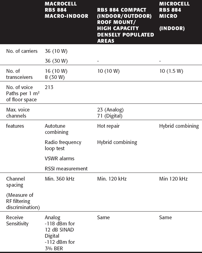
As with IS95 CDMA, here there is a need to support legacy 30 kHz AMPS channels (833×30 kHz channels within a 25 MHz allocation). This implies quite complex combining. The higher the transmitter power, the more channel spacing needed between RF carriers in the combiner. Note also that if any frequency changes are made in the network plan, the combiner needs to be retuned. In this example, the cavity resonators and combiners can be remotely retuned (mechanically activated devices). If there is a power mismatch with the antenna because of a problem, for example, with the feeder, then this is reflected (literally) in the voltage standing wave ratio (VSWR) reading and an alarm is raised.

The receiver sensitivity is specified both for the analog radio channels and the digital channels. 12-dB SINAD is theoretically equivalent to 3 percent BER. This shows that these are really quite complex hardware platforms with fans (and usually air conditioning in the hut), motors (to drive the autotune combiners), and resonators—RF plumbing overhead. These products absorb what is called in the United States windshield time—time taken by engineers to drive out to remote sites to investigate RF performance problems.

In the late 1980s in the United Kingdom, Cellnet used to regularly need to change the frequency plan of the E-TACS cellular network (similar to AMPS) to accommodate additional capacity. This could involve hundreds of engineers making site visits to retune or replace base station RF hardware—the cost of needing to manage lots of narrowband RF channels.

3G Node B Design Objectives

It has been a major design objective in 3G design to simplify the RF hardware platform in order to reduce these costs. As with the handset, it is only necessary to support twelve 5 MHz paired channels and potentially seven 5 MHz nonpaired channels in the IMT2000 allocated band instead of the hundreds of channels in AMPS, TDMA, or GSM.

Unfortunately, of course, many Node Bs will need to continue to support backward compatibility. Broadband linear amplifiers and software configurable radios are probably the best solution for these multimode multiband Node Bs. We look at the RF architecture of a broadband software radio Node B in a case study later in this chapter.

2G Base Stations as a Form Factor and Power Budget Benchmark

In the meantime, customer expectations move on. Over the past 5 years, GSM base stations have become smaller and smaller. Ericsson's pico base station is one example, taking the same amount of power as a lightbulb. Nokia's in-site picocellular reduces form factor further (an A4 footprint).

And even smaller GSM base station products are beginning to appear. The example in Figure 11.2 weighs less than 2 kg and consumes less than 15 W of power.

The continuing reduction of the form factor of 2G base stations represents a challenge for the 3G Node B designer. Vendors need to have a small Node B in the product portfolio for in-building applications. The general consensus between designers is that this should be a single 5 MHz RF carrier Node B weighing less than 30 kg, occupying less than 30 liters. The example shown in Figure 11.3 meets these design requirements. This is a pole-mounted transceiver and as such may be described as having no footprint. It is convection cooled, consuming 500 W for a 10 W RF output and is 500 mm high.

Figure 11.2 Nano base stations (GSM–2G) from ip.access (www.ipaccess.com).

Node B Antenna Configuration

The Node B hardware determines the antenna configuration. The Siemens/NEC Node B shown in Figure 11.3 can either be used on its own supporting one omnidirectional antenna (1×360°) or with three units mounted on a pole to support a three-sector site (3×120° beamwidth antennas).

All other Node Bs in this particular vendor's range at time of writing are floor mounted, mainly because they are too heavy to wall mount or pole mount. The example shown in Figure 11.4 weighs 900 kg and occupies a footprint of 600×450 mm and is 90 cm high. It can support two carriers across three sectors with up to 30 W per carrier, sufficient to support 384 voice channels.

The same product can be double-stacked with a GSM transceiver to give a 1 + 1 + 1 + 6 configuration, one 5 MHz RF carrier per sector for UMTS and a 6 RF carrier GSM BTS, which would typically be configured with 2×200 kHz RF channels per sector. The combined weight of both transceivers is 1800 kg and combined power consumption is over 2 kW.

A final option is to use one of the family of Node Bs illustrated in Figure 11.5. These can be configured to support omnis (360°), four sector (4×90° beamwidth antennas), or six sector (6×60°), with RF power outputs ranging from 6 W to 60 W per RF carrier.

Figure 11.3 Siemens/NEC Node B (UMTS).

The configuration can also support omni transmit and sectorized receive (OTSR), which has the benefit of providing better receive sensitivity. The physical size is 600×450 mm (footprint) by 1400 mm high, and the weight is 1380 kg. Outdoor and indoor versions are available.

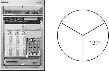
Figure 11.4 Siemens/NEC NB420 Macro Node B.

Figure 11.5 Siemens/NEC NB440 Macro Node B–more sectors, more RF carriers, smaller footprint.

The Benefits of Sectorization and Downtilt Antennas

Sectorization helps to provide more capacity and delivers a better downlink RF link budget (more directivity) and better uplink selectivity (which improves sensitivity). Many Node Bs also use electrical downtilt. We discuss smart antennas in Chapter 13; these antennas can adaptively change the coverage footprint of an antenna either to null out unwanted interference or to minimize interference to other users or other adjacent Node Bs. Electrical downtilt has been used in GSM base stations from the mid-1990s (1995 onward). By changing the elevation of the antenna or the electrical phasing, the vertical beam pattern can be raised or lowered. Figure 11.6 shows how the beam pattern can be adjusted to increase or decrease the cell radius. This can be used to reduce or increase the traffic loading on the cell by reducing or increasing the physical footprint available from the Node B. Adaptive downtilt can be used to change coverage as loading shifts through the day—for example, to accommodate morning rush hour traffic flows or evening rush hour loading.

For in-building coverage, an additional option is to have a distributed RF solution in which a Node B is positioned in a building and then the incoming/outgoing RF signals are piped over either copper feeder (rather lossy) or optical fiber to distributed antennas. The optical fiber option is preferable in terms of performance but requires linear lasers to take the (analog) RF signal and modulate it onto the optical fiber and a linear laser to remodulate the optical signal back to RF at the antenna.

Figure 11.6 Electrical downtilt.

As we shall see in our next section on system planning, the 3G air interface is well suited to a fairly dense low-powered network (less noise rise is produced by adjacent Node Bs and less interference is visible at the Node B receiver). This places a premium on the need to design a small form factor (sub-30 kg) Node B product.

Node B RF Form Factor and RF Performance

Given that operators may be asked to share access hardware and given that operators have been allocated different RF carriers, it may also be necessary to produce small form factor Node Bs capable of processing more than one×5 MHz RF carrier—ideally 60 MHz, though this is at present unrealistic in terms of digital sampling techniques.

The two major design challenges for Node B products are transmit linearity, including the ability to handle multiple downlink OVSF codes per user, and receive sensitivity, including the ability to handle multiple uplink OVSF codes per user. We have said that receive sensitivity can be improved by using electronic downtilt (reducing the exposure of the Node B to visible interference) and multiuser detection where the Node B uses the short codes embedded in each individual handset's offered traffic stream to cancel out unwanted interference energy. Multiuser detection is a longer-term upgrade (rather like frequency hopping was in GSM in the early 1990s).

Receive sensitivity is also a product of how well the radio planning in the network has been done and how well the Node B sites have been placed in relation to the offered traffic. We address these issues in the next section.

As with handsets, RF power budgets can be reduced by increasing processor overhead. For example, we can implement adaptive smart antennas on a Node B, which will provide significant uplink and downlink gain (potentially 20 or 25 dB). This reduces the amount of RF power needed on the downlink and RF power needed on the uplink. However, if the processor power consumption involved (to support the many MIPS of processing required) is high compared to the RF power saved, then very little overall gain would have been achieved. You will just have spent a lot of money on expensive DSPs.

As with handset design, DSPs can do much of the heavy lifting at bit level and symbol level but run out of steam at chip level. There is also a need for substantial parallel processing to support multiple users, each with multiple uplink and downlink OVSF code streams. These factors presently determine existing Node B form factor and functionality. The design objective has to be to balance good practical RF design with judicious use of DSPs and ASICs to deliver power-efficient processor gain. The requirement, as with GSM, is to keep power consumption for small Node Bs in the region of tens of Watts. This means it is easy to install Node Bs indoors without greatly adding to the landlord/hosting energy bill, and for outdoor applications, it provides the basis for solar-powered or wind-powered base station/Node B implementation.

Simplified Installation

IMT2000DS indoor picocells do not need to have a GPS reference. They can be reclocked by handsets moving into the building. This makes installation substantially easier. An engineer can walk into a building, fix a node B to the wall, plug it into a mains power outlet, plug it into a telephone line (the Node B has its own ADSL modem), turn it on, and walk way. If GPS was needed, the engineer would have to pipe a connection to a window so that the GPS antenna could see the sky. Small Node Bs do not incur the same neighborhood resentment as larger Node Bs (for one reason, they do not look like base stations), and the site is sometimes provided for free by the landlord, which is rarely the case for large outdoor sites.

Radio planning, as we will see later in this chapter, is also partly determined by the product mix of Node Bs available from each vendor. Typically, power outputs will be 40 W, 20 W, 10 W, 5 W, or less. Although some planners would argue the case for smaller numbers of larger, more powerful Node Bs, this goes against existing product and installation trends, which clearly point toward the need to maintain a small form factor (small volume/low weight). This in turn determines the choice of architecture used in the Node B design.

Node B Receiver Transmitter Implementation

In Chapters 2 and 3 we discussed the suitability of the digitally sampled IF superhet and the direct conversion receiver architecture for handset implementation. We concluded that either configuration was capable of meeting the handset specification but that longer term, the DCR (or near-zero IF) could show a reduction in component count—especially in multistandard environments—although problems of DC offsets required considerable DSP power (baseband compensation).

The 3G Receiver

We also reviewed transmitter implementation and concluded that the architecture (OPLL) developed for cost reduction/multiband requirements in 2G could show similar benefits in 3G if the problem of processing both amplitude and phase components in the modulation (HPSK) could be overcome. We will now consider receiver and transmitter requirements in Node B implementation and assess whether the architectures discussed in the previous chapters are also suitable for Node B designs.

The Digitally Sampled IF Superhet

In analyzing the handset receiver/transmitter options, we recognized that the prime constraint on any decision was that of battery power requirement. To provide for the handset to access any of the 5 MHz channels in the 60 MHz spectrum allocation, a receiver front end tuning with a 12-step synthesizer is necessary to downconvert the selected channel to be passed through a 5 MHz bandwidth IF centered filter to the sampling ADC. The digitized single 5 MHz channel is then processed digitally to retrieve the source-coded baseband signal. This single-channel approach is adopted in the handset in order to comply with the low-power criteria.

If this single-channel approach were adopted in the Node B, where multiple RF channels may simultaneously be required, the requisite number of receivers would have to be installed. As the restriction of Node B power consumption is not as severe, an alternative approach can be considered.

The ideal approach is to implement a wideband front end, to downconvert the 12 5 MHz-wide channels, to pass a number (or all) of the channels through a wideband IF filter, and to sample and digitize this wider bandwidth of channels. The digitized channels would then be passed to a powerful digital processing capability that could simultaneously extract the downconverted baseband signals. The number of channels to be simultaneously processed would again be dependent on the power available both in implementing an RF front end of sufficient dynamic range and an ADC/DSP combination of sufficient processing capability.

Additionally, a greater dynamic range is required by the ADC and DSP, since in the multichannel environment, the channels may be at substantially different signal strengths and so dynamic range control cannot be used. If the IF gain were to be reduced by a strong signal channel, a weak signal channel would disappear into the noise floor.

The Direct Conversion Receiver (DCR)

We have demonstrated that the DCR is a suitable receiver configuration for single-channel operation in the handset. It is similarly suitable for single-channel operation in the Node B.

How will it perform in the multichannel environment?

Consider a wideband approach to receive four simultaneous channels. The receiver front end would still have a bandwidth of 60 MHz—to be able to operate across all 12 W-CDMA channels. The tuning front end would require a local oscillator (LO) having three discrete frequencies in order to downconvert the band in three blocks of four channels each. In the multicarrier receiver, the LO would be placed in the center of the four channels to be downconverted (received), as shown in Figure 11.7.

The output of the I and Q mixers would be the four channel blocks centered around 0 Hz each time the LO was stepped, as shown in Figure 11.8. A typical IC mixer having a Gilbert cell configuration can only achieve at best an IQ balance of some 25 to 30 dB. This means that if the channel 2 to channel 3 amplitude difference is greater than 30 dB, signal energy from channel 3 will transfer into, and hence corrupt, channel 2. Similarly, there will be an interaction between channels 1 and 4.

If we consider the problem of IQ imbalance, we find there are several causes. Typical causes are those of IC manufacturing and process tolerance, variation with supply voltage to the mixers, temperature variation, and other similar effects. This group of causes are predictable, constant effects that can be characterized at the production test stage and compensating factors inserted into the receive processing software.

Compensation can be affected in the digital processing stages by a process of vector rotation, feeding some Q signal into I, or I into Q as required to balance the system. The greater problem is that of IQ imbalance due to dynamic signal variation effects. These are unbalancing effects that cause the operating point of the mixers to shift with signal strength and radiated signal reflection and reentry effects. These effects have been described in Chapter 2 in our discussion of DC offset problems.

Figure 11.7 Local oscillator positioning for down conversion of channels 1 to 4.

Figure 11.8 Channels 1 to 4 positioned around 0 Hz at mixer outputs.

Although the correction by vector rotation is a relatively simple digital process, the difficulty lies in estimating the instantaneous degree of compensation required given all the variables causing signal amplitude variation. For this reason, the DCR (and near-zero IF) is not chosen for Node B designs. However, the designer should always review the current capability of this technology at the start of any new design, as research is certainly being undertaken to increase the application of the DCR.

The 3G Transmitter

We have considered possible transmitter configurations in Chapter 2, and in Chapter 3, we introduced the need for improved linearity for handset (uplink) modulation. The uplink modulation is HPSK, and this requires considerable linearity to be engineered into the PA. The cost, as always, is increased power consumption. The need for Power-Added Efficiency (PAE) in the handset limits the options that can be used to provide linearity. The additional power available to us in the Node B provides us with a wider number of options.

The RF/IF Section

The application of a linear PA in Node B design should be considered. The downlink signal has QPSK modulation and so has greater amplitude variation than the uplink HPSK. Accordingly, greater linearity is required. There is also the issue of a wideband (multichannel) versus a narrowband (single-channel) approach.

In the Node B we have the option of using 12 separate RF transmitters for the 12 channels and combining their outputs at high power prior to the antenna feed, or, we can create a multichannel signal at baseband (or IF) and pass the composite signal through one high dynamic range, high linearity, high power amplifier. There is a large amount of information, analysis, discussion, and speculation of the benefits of one approach or the other, so we can confine ourselves to a review of linearizing options.

Envelope Elimination and Restoration (EER) and Cartesian approaches were introduced in Chapter 3, so we will consider briefly other alternatives.

Linearization methods fall broadly into two categories:

• Those that use a feedback correction loop operating at the modulation rate.
• Those that use a feedback correction process to update a feed-forward correction process, operating at a slower than modulation rate.

The former method is not particularly well suited to the wide modulation bandwidth of 3G (5 MHz for a single channel and up to 60 MHz for a multicarrier Node B).

Whilst it is relatively simple to extract the envelope from the input RF signal and limit the signal to give a constant envelope drive, there is some advantage to implementing this polar split at the signal generation stage within the DSP.

In particular, it is highly likely that the transfer function through the envelope amplifier and bias/supply modulation process will be nonlinear, and that the drive envelope function will need to be pre-distorted to compensate for this error. The predistortion factors can be held in a lookup table within the DSP, for example, and updated if necessary by some slow feedback loop from the transmitter output.

The EER approach can yield modest improvements in linearity for quite good efficiency (provided the envelope modulation amplifier efficiency is good). The modulation envelope bandwidth for W-CDMA is, however, quite large (approximately 5×5 MHz to include key harmonics), and the efficiency of switched mode modulation amplifiers falls off quite quickly at high switching rates.

Another method to be considered is RF synthesis. A synthesis engine converts the I and Q (Cartesian) representation of the modulation waveform into two frequency and phase modulated components, the vector sum of which is identical to the source signal (see Figure 11.9). Amplification of these two constant envelope waveforms is performed using Class C or Class F/S switching amplifiers for maximum efficiency, and the outputs are combined to give the composite high-power RF synthesized waveform. One of the key challenges with RF synthesis is the combination of these two high-power FM signals without losing much of the power in the combiner process.

The vector diagram in Figure 11.10 shows how the output signal is synthesized from the summation of the two constant envelope rotating vectors. Full output power occurs when the two vectors are in phase. Minimum output power is synthesized when the two vectors are 180 degrees out of phase. Using a DSP to generate the two constant envelope phase modulated components is quite feasible, since the algorithm is simple. The processing rate, however, must be very high to accommodate the bandwidth expansion of the nonlinear function involved, and the sample rate of the ADCs must also accommodate the bandwidth expansion of the FM modulated outputs. These high sampling rates and the corresponding high power consumption of the DSP and ADC components means that this approach is only feasible for nonportable applications at the present time.

Figure 11.9 Basic RF synthesis operation.

Figure 11.10 RF synthesis vector diagram.

A large number of amplifier linearization solutions are based on predistortion of the signal driving the amplifier in an attempt to match the nonlinear transfer characteristic of the amplifier with an inverse characteristic in the predistortion process. The challenge with predistortion is to be able to realize a predistortion element that is a good match to the inverse of the amplifier distortion—that is, low cost and low power in its implementation—and that can, if necessary, be adapted to track changes in the amplifier response with time, temperature, voltage, device, operating frequency, operating power point, and Voltage Standing Wave Ratio (VSWR).

For complex envelope modulation formats such as multicarrier W-CDMA, the envelope excursions of the composite waveform will cause the amplifier to operate over its full output range. This means that a predistorter element must also match this characteristic over a wide range of input levels if high levels of linearity are to be achieved.

With a typical superhet design of transmitter, there are three locations where pre-distortion can be implemented. The options are shown in Figure 11.11. An RF solution is attractive, since it is likely to be small and does not require modification of the remainder of the transmit stages. An IF solution is likely to make fabrication of an adaptive predistortion element more practical. A baseband DSP based solution will give ultimate flexibility in implementation, but is likely to take a significant amount of processor cycles and hence consume most power.

One of the simplest RF predistorters to implement is a third-order predistorter. Recognizing that much of the distortion in an amplifier is generated by third-order nonlinear effects, a circuit that creates third-order distortion—for example, a pair of multipliers—can be used to generate this type of distortion but in antiphase. When summed with the drive to the amplifier, significant reduction in the third-order products from the amplifier output can be achieved. Of course, good performance relies on close matching to the gain and phase of the third-order distortion for a particular device, and without some form of feedback control of these parameters, only limited correction is possible over a spread of devices and operating conditions.

Figure 11.11 Location for predistorter components.

It would be very simple to construct an open-loop DSP-based predistorter using a lookup table; however, for most applications, the characteristics of the transmitter device changes so much with operating point that some form of updating of the pre-distortion function is needed. As soon as an adaptive control process is introduced, ADC components are needed, additional DSP processing used, reliable and rapid convergence control algorithms must be identified, and the whole process becomes quite complicated. Within a DSP, it is possible to create any predistortion characteristic required and rapidly update the transfer function to follow changes in the amplifier device response.

As the cost and power consumption of DSP engines continues to fall and the processing power increases, the digital baseband predistortion solution becomes more and more attractive—first for Node B use but also for portable use. There are two main options for updating a predistortion lookup table: using power indexing, which involves a one-dimensional lookup table, or Cartesian (I/Q) indexing, giving rise to a two-dimensional lookup table.

Power indexing will result in a smaller overall table size and faster adaptation time, since the number of elements to update is smaller. It does not, however, correct AM-PM distortion, which means that only limited linearization is possible. I/Q indexing will provide correction for both AM-AM and AM-PM distortion and so give optimum results, but the tables are large and adaptation time slow. For wideband multicarrier signals it is necessary for the lookup table to have a frequency-dependant element to accommodate frequency-dependent distortion through the amplifier chain. This can give rise to three-dimensional tables.

In summary, baseband digital predistortion is the most versatile form of predistortion and will become more widely used as the cost and power consumption of DSP falls. Because of the slow adaptation time for a lookup table predistorter, it is not possible to correct for the memory effect in high-power amplifiers, and so this will limit the gain for multicarrier wideband applications. Correct choice of lookup table indexing will give faster adaptation rates and smaller table size; however, frequency dependent effects in the amplifier cannot be ignored.

An alternative to using a lookup table is to synthesize in real time the predistorter function, much like the third-, fifth-, and seventh-order elements suggested for RF predistortion. This shifts the emphasis from lookup table size to processor cycles, which may be advantageous in some cases.

The final linearization method to be considered is the RF feed-forward correction system. This technique is used widely for the current generation of highly linear multicarrier amplifiers designs in use today, and there are many algorithm devices for correcting the parameters in the feed-forward control loops. More recently, combinations of feed forward and predistortion have appeared in an attempt to increase amplifier efficiency by shifting more of the emphasis on pre-correction rather than post-correction of distortion.

A feed-forward amplifier operates by subtracting a low-level undistorted version of the input signal from the output of the main power amplifier (top path) to yield an error signal that predominantly consists of the distortion elements generated within the amplifier. This distortion signal itself is amplified and then added in antiphase to the main amplifier output in an attempt to cancel out the distortion components.

Very careful alignment of the gain and phase of the signals within a feed-forward linearization system is needed to ensure correct cancellation of the key signals at the input to the error amplifier and the final output of the main amplifier. This alignment involves both pure delay elements to offset delays through the active components, as well as independently controlled gain and phase blocks. The delay elements in particular must be carefully designed, since they introduce loss in the main amplifier path, which directly affects the efficiency of the solution. Adaptation of the gain and phase elements requires a real-time measurement of the amplifier distortion and suitable processing to generate the correct weighting signals. Most feed-forward amplifiers now use DSP for this task. Where very high levels of linearity are needed, it is possible to add further control loops around the main amplifier. Each subsequent control loop attempts to correct for the residual distortion from the previous control loop, with the result that very high levels of linearity are possible but at the expense of power-added efficiency through the amplifier. Feed-forward control requirements are shown in Figure 11.12.

In summary, feed-forward amplifiers can deliver very high levels of linearity over wide operating bandwidth and can operate as RF-in, RF-out devices, making them attractive standalone solutions. Their main drawback is the relatively poor efficiency. Many new multicarrier amplifier solutions are utilizing predistortion correction techniques to try and reduce the load on the feed-forward correction process so that it can operate in a single-loop mode with good main amplifier efficiency. The poor efficiency makes feed forward an unlikely candidate for handset applications; however, since these tend to operate only in single-carrier mode, predistortion techniques alone are likely to give sufficient gain.

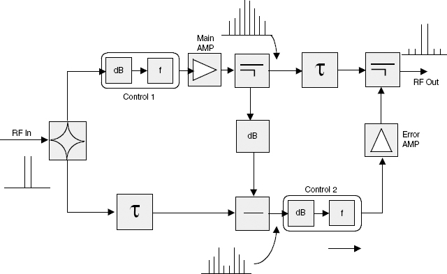
Figure 11.12 Feed-forward control requirements.

The Baseband Section

In Chapter 3 we discussed code generation requirements and root raised cosine filter implementation, and we introduced digital processing methods of producing these functions in the handset. These same functions are required in the Node B transmitter, but given less restriction on power consumption, different trade-offs of software against configured silicon may be made. Also, in the handset it was seen that after the RRC filter implementation, the signals (I and Q) were passed to matched DACs for conversion into the analog domain. An analog-modulated IF was produced that was then upconverted to final transmit frequency. Again, in the Node B, the signal can remain in the digital domain—to produce a modulated IF and only be converted to analog form prior to upconversion. This approach comes nearer to the software radio concept and so provides greater flexibility.

Interpolation

The baseband signal that has been processed up to this stage (RRC filtering) has been constructed at a sample rate that meets the Nyquist criteria for its frequency content. Ultimately, in this example, the signal will be digitally modulated and the IQ streams recombined to yield a real digital intermediate frequency. This will then be applied to a digital-to-analog converter to give a modulated analog IF suitable for upconversion to the final carrier frequency. Because the digital frequency content is increasing (digital upconversion and IQ combining), the sample rate must be increased to re-meet the Nyquist requirement. This is the process of interpolation—the insertion of additional samples to represent the increased frequency components of the signal.

QPSK Modulation

Channels are selected in the digital domain using a numerically controlled oscillator (NCO) and digital mixers. Direct digital synthesis gives more precise frequency selection and shorter settling time; it also provides good amplitude and phase balance. The digital filter provides extremely linear phase and a very good shape factor. Figure 11.13 reminds us of the processing blocks.

Figure 11.13 Positioning of the NCO.

W-CDMA requirements are as follows:

• Nyquist filter
  • Root raised cosine filter: α = 0.22
  • Sampling rate: 3.84 Msps×4
• NCO
  • 60 MHz bandwidth for channel mapping
  • High spurious free dynamic range (SFDR)

The highest rate processing function in the baseband transmitter is the pulse shaping and vector modulation. These tasks must therefore be designed with care to minimize processing overhead and hence power consumption and chip size. A design example from Xilinx for a Node B unit employs an eight times oversampling approach. (Sample rate is eight times symbol rate.) The output frequency for the channel is set using a digital NCO (lookup table method).

The interpolation process is performed using the RRC filter as the first interpolator filter, with a factor of eight sample rate increase. This is followed by two half-band factor of two interpolators, fully exploiting the zero coefficient property of the half-band filter design.

Because the sample rate at the input to the filters is already very high to accommodate the 3.84 Mcps spread signal, the processing for all three filters is significant. With a total of 3.87 billion MACs used for the I and Q channels, this task alone represents about 38 times the processing load for a second-generation GSM phone.

The use of a digital IF design such as this is clearly not feasible for handset implementation with current technology, since the power consumption of the DSP engines would be too high. Even for Node B use, the approach is using approximately 25 percent of a top-end Virtex 2 FPGA.

Technology Trends

In this and earlier chapters we have seen the need for a dramatic increase in baseband processing capability in the 3G standards. Even a minimum-feature entry-level handset or Node B requires several orders more digital processing than has been seen in 2G products.

It may be argued that it is the practical restrictions of digital processing capability and speed versus power consumption that will be the prime factor in restricting introduction and uptake rate of 3G networks and services. It is not surprising, therefore, that most established and many embryo semiconductor, software, fabless, and advanced technology houses are laying claim to having an ideal/unique offering in this area. Certainly, design engineers facing these digital challenges need to constantly update their knowledge of possible solutions.

Advanced, full-capability handsets and node Bs using smart antennas, multiuser detection and, multiple code, and channel capability will require increasingly innovative technologies. Solutions offered and proposed include optimized semiconductor processes, both in scale and materials (for example, SiGe, InP, and SiC), Micro-Electro-Mechanical Systems (MEMS), cluster DSPs, reconfigurable DSPs, wireless DSP, and even an optical digital signal processing engine (ODSPE) using lenses, mirrors, light modulators, and detectors. The designer will not only need to weigh the technical capabilities of these products against the target specification but also weigh the commercial viability of the companies offering these solutions.

System Planning

We have considered some of the factors determining Node B RF power and downlink quality (for example, linearity) and Node B receive sensitivity (uplink quality). We now need to consider some of the system-level aspects of system planning in a 3G network.

Many excellent books on system planning are available. Several have been published by Wiley and are referenced in Table 11.8.

Our purpose in this chapter is to put simulation and planning into some kind of historical perspective. Why is it that simulations always seem to suggest that a new technology will work rather better than it actually does in practice? Why is it that initial link budget projections always seem to end up being rather overoptimistic.

Cellular technologies have a 15-year maturation cycles. Analog cellular technologies were introduced in the 1980s and didn't work very well for five years (the pain phase). From the mid-1980s onward, analog cellular phones worked rather well, and by 1992 (when GSM was introduced), the ETACS networks in the United Kingdom and AMPS networks in the United States and Asia were delivering good-quality consistent voice services with quite acceptable coverage. The mid-1980s to early 1990s were the pleasure phase for analog. In the early 1990s there were proposals to upgrade ETACS in the United Kingdom (ETACS 2) with additional signaling bandwidth to improve handover performance. In the United States, narrowband (10 kHz channel spacing) AMPS was introduced to deliver capacity gain. However, the technology started running out of improvement potential, and engineers got bored with working on it. We describe this as the perfection phase.

When GSM was introduced in 1992, it really didn't work very well. Voice quality was, if anything, inferior to the analog phones and coverage was poor. The next five years were the pain phase. GSM did not start to deliver consistent good-quality voice service until certainly 1995 and arguably 1997.

Table 11.8 Further Reading

The same is happening with 3G. Networks being implemented today (2002 to 2003) will not deliver good, consistent video quality until at least 2005 and probably not until 2007. By that time, 2G technologies (GSM US TDMA) will be fading in terms of their further development potential, and a rapid adoption shift will occur.

Let's look at this process in more detail.

The Performance/Bandwidth Trade-Off in 1G and 2G Cellular Networks

The AMPS/ETACS analog cellular radio networks introduced in the 1980s used very well established baseband and RF processing techniques. The analog voice stream was captured using the variable voltage produced by the microphone, companded and pre-emphasized, and then FM modulated onto a 25 kHz (ETACS) or 30 kHz (AMPS) radio channel.

The old 1200-bit rate FFSK signaling used in trunked radio systems in the 1970s was replaced with 8 kbps PSK (TACS) or 10 kbps PSK for AMPS. (As a reminder, AMPS stands for Advanced Mobile Phone System, TACS for Total Access Communications System, and E-TACS for Extended TACS—33 MHz rather than 25 MHz allocation.)

At the same time (the Scandinavians would claim earlier), a similar system was deployed in the Nordic countries known as Nordic Mobile Telephone System (NMT). This was a narrowband 12½ kHz FM system at 450 MHz.

All three first-generation cellular systems supported automatic handover as a handset moved from base station to base station in a wide area network. The handsets could be instructed to change RF channel and to increase or decrease RF power to compensate for the near/far effect (whether the handset was close or far away from the base station). We have been using the past tense, but in practice, AMPS phones are still in use, as well as some, though now few, NMT phones.

Power control and handover decisions were taken at the MSC on the basis of channel measurements. AMPS/ETACS both used supervisory audio tones. These were three tones at 5970, 6000, and 6030 Hz (above the audio passband). One of the three tones would be superimposed on top of the modulated voice carrier. The tone effectively distinguished which base station was being seen by the mobile. The mobile then retransmitted the same SAT tone back to the base station. The base station measured the signal-to-noise ratio of the SAT tone and either power-controlled the handset or instructed the handset to move to another RF channel or another base station. Instructions were sent to the mobile by blanking out the audio path and sending a burst of 8-kbps PSK signaling.

This still is a very simple and robust system for managing handsets in a mobile environment. However, as network density increased, RF planning became quite complicated (833 channels to manage in AMPS, 1321 channels to manage in ETACS), and there was insufficient distance between the SAT tones to differentiate lots of different base stations being placed relatively close to one another. There were only three SAT tones, so it was very easy for a handset to see the same SAT tone from more than one base station.

Given that the SAT tones were the basis of power control and handover decisions, the network effectively became capacity-limited in terms of its signaling bandwidth.

The TDMA networks (GSM and IS136 TDMA) address this limitation by increasing signaling bandwidth. This has a cost (bandwidth overhead) but delivers tighter power and handover control.

For example: In GSM, 61 percent of the channel bandwidth is used for channel coding and signaling, as follows:

The SACCH (slow associated control channel) is used every thirteenth frame to provide the basis for a measurement report. This is sent to the BTS and then on to the BSC to provide the information needed for power control and handover. Even so, this is quite a relaxed control loop with a response time of typically 500 ms (twice a second), compared to 1500 times a second in W-CDMA (IMT2000DS) and 800 times a second in CDMA2000.

The gain at system level in GSM over and above analog cellular is therefore a product of a number of factors: 1. There is some source coding gain in the voice codec. 2. There is some coherence bandwidth gain by virtue of using a 200 kHz RF channel rather than a 25 kHz channel. 3. There is some channel coding gain by virtue of the block coding and convolutional coding (achieved at a very high price with a coding overhead of nearly 10 kbps). and 4. There is a gain in terms of better power control and handover.

In analog TACS or AMPS, neighboring base stations measure the signal transmission from a handset and transfer the measurement information to the local switch for processing to make decisions on power control and handover. The information is then downloaded to the handset via the host base station. In an analog network being used close to capacity, this can result in a high signaling load on the links between the base stations and switches and a high processing load on the switch.

In GSM, the handset uses the six spare time slots in a frame to measure the received signal strength on a broadcast control channel (BCCH) from its own and five surrounding base stations. The handset then preprocesses the measurements by averaging them over a SACCH block and making a measurement report. The report is then retransmitted to the BTS using an idle SACCH frame. The handset needs to identify co-channel interference and therefore has to synchronize and demodulate data on the BCCH to extract the base station identity code, which is then included in the measurement report. The handset performs base station identification during the idle SACCH.

The measurement report includes an estimate of the bit error rate of the traffic channels using information from the training sequence/channel equalizer. The combined information provides the basis for an assessment of link quality degradation due to co-channel and time dispersion and allows the network to make reasonably accurate power control and handover decisions.

Given the preceding information, various simulations were done in the late 1980s to show how capacity could be improved by implementing GSM. The results of base simulations were widely published in the early 1990s. Table 11.9 suggests that additional capacity could be delivered by increasing the reuse ratio (how aggressively frequencies were reused within the network) from 7 to 4 (the same frequency could be reused every fourth cell). The capacity gain could then be expressed in Erlangs/sq km.

In practice, this all depended on what carrier-to-interference ratio was needed in order to deliver good consistent-quality voice. The design criteria for analog cellular was that a C/I of 18 dB was needed to deliver acceptable speed quality. The simulations suggested GSM without frequency hopping would need 11 dB, which would reduce to 9 dB when frequency hopping was used. In practice, these capacity gains initially proved rather illusory partly because, although the analog cellular networks were supposed to be working at an 18 dB C/I, they were often working (really quite adequately) at C/Is close to 5—that is, there was a substantial gap between theory and reality.

The same reality gap happened with coverage predictions. The link budget calculations for GSM were really rather overoptimistic, particularly because the handsets and base station hardly met the basic conformance specification.

Through the 1990s, the sensitivity of handsets improved, over and above the conformance specification, typically by 1 dB per year. Similarly, base station sensitivity increased by about 3 or 4 dB. This effectively delivered coverage gain. Capacity gain was achieved by optimizing power control and handover so that dropped call performance could be kept within acceptable limits even for relatively fast mobility users in relatively dense networks. Capacity gain was also achieved by allocating 75 MHz of additional bandwidth at 1800 MHz. This meant that GSM 900 and 1800 MHz together had 195 + 375 × 200 kHz RF channels available between 4 network operators, 570 RF channels each with 8 time slots = 4640 channels! GSM networks have really never been capacity-limited. The capacity just happens sometimes to be in the wrong place. Cellular networks in general tend to be power-limited rather than bandwidth-limited.

Table 11.9 Capacity Gain Simulations for GSM

So it was power, or specifically coverage, rather than capacity that created a problem for GSM 1800 operators. As frequency increases, propagation loss increases. It also gets harder to predict signal strength. This is because as frequency increases, there is more refraction loss—radio waves losing energy as they are reflected from buildings or building edges. GSM 1800 operators needed to take into account at least an extra 6 dB of free space loss over and above the 900 MHz operators and an additional 1 to 2 dB for additional (hard to predict) losses. This effectively meant a network density four to five times greater than the GSM 900 operators needed to deliver equivalent coverage. The good news was that the higher frequency allowed more compact base station antennas, which could also potentially provide higher gain. The higher frequency also allowed more aggressive frequency reuse; though since capacity was not a problem, this was really not a useful benefit.

It gradually dawned on network operators that they were not actually short of spectrum and that actually there was a bit of a spectral glut. Adding 60 + 60 MHz of IMT2000 spectrum to the pot just increased the oversupply. Bandwidth effectively became a liability rather than an asset (and remains so today).

This has at last shifted attention quite rightly away from capacity as the main design objective. The focus today is on how to use the limited amount of RF power we have available on the downlink and uplink to give acceptable channel quality to deliver an acceptably consistent rich media user experience.

TDMA/CDMA System Planning Comparisons

In GSM or US TDMA networks, we have said that the handset produces a measurement report that is then sent to the BSC to provide the basis for power control and handover. The handset does radio power measurements typically every half second (actually, 480 ms) and measures its own serving base station and up to five other base stations in neighboring cells. This is the basis of Mobile-Assisted HandOff (MAHO).

This measurement process has had to be modified as GPRS has been introduced. GPRS uses an adaptive coding scheme—CS1, 2, 3, or 4, depending on how far the handset is away from the base station. The decision on which coding scheme to use is driven by the need to measure link quality. Link quality measurement can only be performed during idle bursts. In voice networks, the measurement has traditionally been done every 480 ms. The fastest possible measurement rate is once every 120 ms (once every multiframe), which is not fast enough to support adaptive coding.

IN E-GPRS (GPRS with EDGE), measurements are taken on each and every burst within the equalizer of the terminal resulting in an estimate of the bit error probability (BEP). The BEP provides a measure of the C/I on a burst-by-burst basis and also provides information on the delay spread introduced by the channel and the velocity (mobility) of the handset—that is, how fast the handset/mobile is traveling through the multipath fading channel. The variation of BEP value over several bursts also provides information on frequency hopping. A mean BEP is calculated per radio block (four bursts), as well as the variation (the standard deviation of the BEP estimation divided by the mean BEP) over the four bursts. The results are then filtered for all the radio blocks sent within the measurement period.

Figure 11.14 Link adaptation.

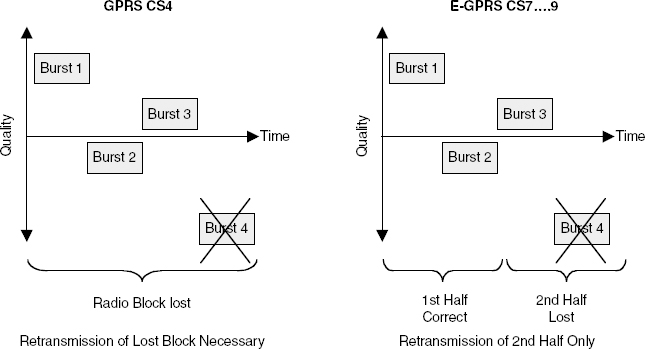
For the higher coding schemes within GPRS (MCS7 to 9), the interleaving procedure is changed. If frequency hopping is used, the radio channel is changing on a per-burst level. Because a radio block is interleaved and transmitted over four bursts for GPRS, each burst may experience a completely different interference environment. If, for example, one of the four bursts is not properly received, the whole radio block will be wrongly decoded and have to be retransmitted. In E-GPRS, the higher coding schemes MCS7, MCS8, and MCS9 transmit two radio blocks over the four bursts. The interleaving occurs over two bursts rather than four, which reduces the number of bursts that need to be transmitted if errors are detected. This is shown in Figure 11.14. The process is known as link adaptation.

These higher coding schemes work better when frequency hopping is used, but you lose the gain delivered from deep interleaving.

Link adaptation uses the radio link quality measurement by the handset on the downlink or base station on the uplink to decide on the channel coding and modulation that should be used. This is in addition to the power control and handover decisions being made. The modulation and coding scheme can be changed every frame (4.615 ms) or four times every 10 ms (the length of a frame in IMT2000).

E-GPRS is effectively adapting to the radio channel four times every 10 ms (at a 400 Hz rate). IMT2000 adapts to the radio channel every time slot, at a 1500 Hz rate. Although the codecs and modulation scheme can theoretically change every four bursts (every radio block), the measurement interval is generally slower.

The coding schemes are grouped into three families: A, B, and C. Depending on the payload size, resegmentation for retransmission is not always possible, thus determining which family of codes are used.

Table 11.10 shows the nine coding schemes used in E-GPRS, including the two modulation schemes (GMSK and 8PSK).

Table 11.10 E-GPRS Channel Coding Schemes

The performance of a handset sending and receiving packet data is therefore defined in terms of throughput, which is a product of the gross throughput less the retransmissions needed. The retransmission will introduce delay and delay variability, which will require buffering. If the delay variability exceeds the available buffer bandwidth, then the packet stream will become nonisochronous, which will cause problems at the application layer.

We can see that it becomes much harder to nail down performance in a packet-routed network.

As we will see in the next section, link budgets are still established on the basis of providing adequate voice quality across the target coverage area. Adaptive coding schemes if well implemented should mean that when users are closer to a base station, data throughput rates can adaptively increase. When a user is at the cell edge, data throughput will be lower, but in theory, bit error rates and retransmission overheads should remain relatively constant.

Having convinced ourselves that this may actually happen, we can now move on to radio system planning.

Radio Planning

With existing TDMA systems it has been relatively simple to derive base station and handset sensitivity. The interference is effectively steady-state. Coverage and capacity constraints can be described in terms of grade of service and are the product of network density.

In IMT2000, planning has to take into account noise rise within a (shared) 5 MHz channel, an allowance for fast power control headroom at the edge of the cell and soft handover gain. The interference margin is typically 1 to 3 dB for coverage-limited conditions and more for capacity-limited networks. Fast power control headroom is typically between 2 and 5 dB for slow-moving handsets. Soft handover gain—effectively uplink and downlink diversity gain—is typically between 2 and 3 dB. There are four power classes. Class 1 and 2 are for mobiles. Class 3 and 4 are for handsets (mobiles would, for example, be vehicle-mounted). These are shown in Table 11.11. Typical maximum power available at a Node B would be 5, 10, 15, 20, or 40 Watts.

In 3GPP, E_b/N_o targets are set that are intended to equate with the required service level. (As mentioned in earlier chapters, E_b/N_o is the energy per bit over the noise floor. It takes into account the channel coding predetermined by the service to be provided.) The E_b/N_o for 144 kbps real-time data is 1.5 dB. The E_b/N_o for 12.2 kbps voice is 5 dB.

Why does E_b/N_o reduce as bit rate increases? Well, as bit rate increases, the control overhead (a fixed 15 kbps overhead) reduces as a percentage of the overall channel rate. In addition, because more power is allocated to the DPCCH (the physical control channel), the channel estimation improves. However, as the bit rate increases, the spreading gain reduces.

IMT2000 planning is sensitive to both the volume of offered traffic and the required service properties of the traffic—the data rate, the bit error rate, the latency, and service-dependent processing gain (expressed as the required E_b/N_o).

System performance is also dependent on system implementation—how well the RAKE receiver adapts to highly variable delay spreads on the channel, how well fast fading power control is implemented, how well soft/softer handover is configured, and interleaving gain.

Downlink capacity can also be determined by OVSF code limitations (including nonorthogonality) and downlink code power. The power of the transmitter is effectively distributed among users in the code domain. 10 W, for example, gets distributed among a certain amount of code channels—the number of code channels available determines the number of users that can be supported. On the uplink, each user has his or her own PA, so this limitation does not apply.

A Node B will be exposed to intracell and intercell interference. Intracell interference is the interference created by the mobiles within the cell and is shown in Figure 11.15.

Table 11.11 Power Classes for Mobiles and Handsets

Figure 11.15 Intracell interference.

Intercell interference is the sum of all the received powers of all mobiles in all other cells and is shown in Figure 11.16.

Figure 11.16 Intercell interference.

Interference from adjacent cells initially exhibits a first-order increase. At a certain point, handsets start increasing their power to combat noise rise, which in turn increases noise rise! A first-order effect becomes a second-order effect; the cell has reached pole capacity. The rule of thumb is that a 50 percent cell load (50 percent pole capacity) will result in 3 dB of intracell interference. A 75 percent cell load implies 6 dB of intracell interference.

In other words, say you have a microcell with one transceiver. It will have a higher data rate handling capability than a macrocell with one transceiver because the microcell will not see so much interference as the macrocell.

Rules of Thumb in Planning

Macrocell performance can be improved by using adaptive downtilt to reduce interference visibility, which in turn will reduce noise rise. However, the downtilt also reduces the coverage footprint of the cell site. The other useful rule of thumb is to try and position Node B sites close to the offered traffic to limit uplink and downlink code power consumption. The effect is to increase cell range. Unfortunately, most sites are chosen pragmatically by real estate site acquisition specialists and are not really in the right place for a 3G network to deliver optimum performance.

Figure 11.17 shows how user geometry (how close users are to the Node B) determines cell footprint. As users move closer to the cell center they absorb less downlink code domain power. This means more code domain power is available for newcomers so the cell footprint grows (right-hand circle). If existing users are relatively distant from the Node B, they absorb more of the Node B's code domain power and the cell radius shrinks (left-hand circle).

Interference and noise rise can be reduced by using sectored antennas and arranging receive nulls in a cloverleaf pattern. Typical Node B configuration might therefore include, say, a single RF carrier omnidirectional antenna site for a lightly populated rural area, a three-sector site for a semi-rural area (using 1×RF carrier per sector), a three-sector site configuration with two RF carriers per sector for urban coverage, or alternatively, an eight-sector configuration with either one or two RF carriers per sector for dense urban applications.

Figure 11.17 Impact of user geometry on cell size.

These configurations are very dependent on whether or not network operators are allowed to share Node B transceivers, in which case four or more 5-MHz RF channels would need to be made available per sector to give one RF channel per operator.

How System Performance Can Be Compromised

System performance can be compromised by loss of orthogonality. OVSF codes, for example, are not particularly robust in dispersive channels (e.g., large macrocells). Degraded orthogonality increases intracell interference and is expressed in radio planning as an orthogonality factor. Orthogonality on the downlink is influenced by how far the users are away from the Node B. The further away they are, the more dispersive the channel and the more delay spread there will be. Loss of orthogonality produces code interference.

We said earlier that we can implement soft handover to improve coverage. Effectively, soft handover gives us uplink and downlink diversity gain; however, soft handover absorbs radio bandwidth and network bandwidth resources, long code energy on the radio physical layer, and Node B to RNC and RNC to RNC transmission bandwidth in the IP RAN. If lots of users are supported in soft handover, range will be optimized, but capacity (radio and network capacity) will be reduced. If very few users are supported on soft handover, range will be reduced, but (radio and network) capacity will increase.

In the radio network subsystem (RNS), the controlling RNC (CRNC) looks after load and congestion control of its own cells, admission control, and code allocation. The drift RNC (DRNC) is any RNC, other than the serving RNC, that controls cells used by the Node B. Node B looks after channel coding and interleaving, rate adaption, spreading, and inner-loop power control.

The RNC looks after combining—the aggregation of multiple uplinks and downlinks. Note that a handset can be simultaneously served by two Node Bs, each of which sends and receives long code energy to and from the handset. In addition, each Node B could be sending and receiving multiple OVSF code streams via two Node Bs to either the CRNC, or if the handset is between RNCs, to both the CRNC and DRNC. The CRNC and DRNC then have to talk to each other, and the CRNC has to decide which long code channel stream to use on a frame-by-frame basis or to combine the two long code channel streams together to maximize combining again. This is a nontrivial decision-making process that will need to be optimized over time. It will take at least 5 years for these soft handover algorithms to be optimized in IMT2000DS networks.

The RNC also has to respond to admission priorities set/predetermined by the admission policy, which is predetermined by individual user or group user service level agreements. The requirements of the traffic (tolerance to delay and delay variability) determine the admission policy and how offered traffic will be distributed between serving cells. There are four service classes in IMT2000. The low-delay data (LDD) services are equivalent to the constant bit rate and variable bit rate services available in ATM and are used to support conversational and streamed video services. The service classes are shown in Table 11.12.

Table 11.12 Classes of 3GPP Service

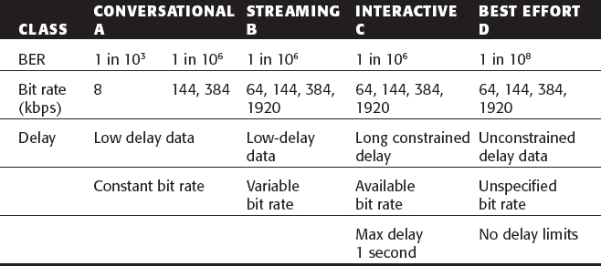
LCD and UDD are equivalent to the available bit rate and unspecified bit rate services available in ATM and are used to support interactive and best-effort services. Low bit error rates can be achieved if data is delay-tolerant. A higher-layer protocol, for example, TCP, detects packet-level error rates and requests a packet retransmission. It is possible to reduce bit error rates. The cost is delay and delay variability.

Link budgets (coverage and capacity planning) are therefore dependent on individual user bit rates, user QoS requirements, propagation conditions, power control, and service class. The offered traffic statistics will determine the noise rise in the cell. For example, a small number of high bit rate users will degrade low bit rate user's performance. The failure to meet these predefined service levels can be defined and described as an outage probability.

The job of the RNC (controlling RNCs and drift RNCs) is to allocate transmission resources to cells as the offered traffic changes. Loading can be balanced between RNCs using the IUR interface. This is known as slow dynamic channel allocation. An RNC balances loading across its own Node Bs over the IUB interface. RF resources (code channels) are allocated by the Node B transceivers. This is described as fast dynamic channel allocation, with the RNC allocating network bandwidth and radio bandwidth resources every 10 ms. Both the network bandwidth and radio bandwidth need to be adaptive. They have to be able to respond to significant peaks in offered traffic loading.

Timing Issues on the Radio Air Interface

We said that radio link budgets can be improved by putting handsets into soft handover. Care must however be taken to maintain time alignment between the serving Node B and soft handover target Node B. Path delay will be different between the two serving Node Bs and will change as the user moves. The downlink timing therefore has to be adjusted from the new serving Node B so that the handset RAKE receiver can coherently combine the downlink signal from each Node B. The new Node B adjusts downlink timing in steps of 256 chips (256×0.26 μs = 66.56 μs) until a short code lock is achieved in the handset. If the adjustment is greater than 10 ms, then the downlink has to be decoded to obtain the system frame number to reclock the second (soft handover) path with the appropriate delay.

Use of Measurement Reports

The measurement report in IMT2000DS does the same job as the measurement report in GSM. It provides the information needed for the Node B to decide on power control or channel coding or for the RNC to decide on soft handover.

In IMT2000DS, the measurement report is based on received signal power. This is the received power on one code after despreading defined on the pilot symbols. The decoded pilot symbols provide the basis for the measurement report, which provides the basis for power control or channel coding and soft handover. It also provides the basis for admission control and load balancing. Effectively, it is providing information on the noise floor as perceived by individual users on individual OVSF/long code channels. It provides additional information over and above wideband noise measurements (which can also be used to set admission control policy).

The measurement report includes E_b/N_o (the received signal code power divided by the total received power), signal-to-interference ratio (which is determined partly by cell orthogonality), and block error rate measurements (used for outer-loop power control).

Load estimation can be done either by measuring wideband received power, which will be the sum of intercell, intracell interference, and background receiver noise, or by measuring throughput, which can be measured in terms of bit rate or E_b/N_o. An additional option would be to measure buffer occupancy. Initially, wideband power estimation is probably an adequate way to decide on admission control and load balance at the RNC.

Cell sizes can be increased or decreased physically by increasing or decreasing downlink transmit power or by physically changing antenna patterns (see Chapter 13). It may, for example, be the case that interference patterns change through the day as traffic changes. The loading and interference from users traveling to work by car in the morning may be different from the loading and interference generated from users traveling home at night. The cell site configuration can be adapted to match the offered traffic (and offered noise) as it changes through the day.

In our later chapter on Service Level Agreements, we review how radio and network performance has to be integrated into provable performance platforms, providing proof that a requested grade of service has been delivered.

At radio system level we need to comprehend a number of factors. One important factor is soft handover gain. This is the effect of the handset serving two Node Bs. It can be considered as a macro diversity factor, both on the uplink and the downlink. Because the ultimate objective of network control is to maintain an acceptable BER, the additional factor of soft handover gain enables the handset transmission power to be decreased, which in turn reduces both the intercell and intracell interference and so may be expressed as a capacity gain. As the effective path gain is increased—by virtue of the aggregate signal up to two Node Bs—but the uplink transmit power is reduced, the receive power to the network remains the same.

However, the receive sensitivity is no longer a constant design factor of the handset but is also dependent on a number of dynamic factors.

Intercell and intracell interference adds to the noise power. Processing gain influences sensitivity. The E_b/N_o needed will vary (with service, data rate, speed, and multipath channel). In addition a fast fading margin needs to be added to account for the deterioration in E_b/N_o caused by power limiting at the cell edge.

The link budget will change depending on mobility factors as a user moves within the cell, as users move in other cells, and as users move into and out of cells. The link budget will also change on the service factor as users change data rate (the service factor).

We also need to take into account processing gain. Processing gain (see Table 11.13) is based on the ratio of the user data rate to the chip rate (whereas spreading gain is the ratio of the channel data rate to the chip rate—see Chapter 3). These figures need to include the coding gain available from convolutional encoding and interleaving. This will vary depending on what convolutional encoding or interleaving is used, which, in turn, is dependent on the service being supported. This is allowed for by changing the required E_b/N_o for each service.

Table 11.14 shows typical E_b/N_os needed for particular services. The E_b/N_o is lower for the UDD service (unconstrained delay). The delay tolerance effectively makes the data easier to send. Services at a higher mobile speed require a higher E_b/N_o because of power control errors (the inability to follow the fast fading envelope at higher speeds means the fade margin has to be increased). Services in rural areas need a higher E_b/N_o because the delay spread (and nonorthogonality) is greater.

Fast fading allows all handsets operating in a cell to have equally received powers at the Node B receiver. Fast fading power control effectively equalizes the fading character of the radio channel so that the receiver sees a Gaussian-like radio channel. The BER versus E_b/N_o will improve in a Gaussian channel. The improvement in E_b/N_o is called the fast power control gain.

Table 11.13 Link Budget Processing Gain

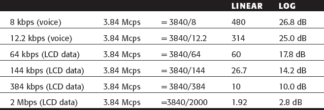
Table 11.14 Example E_b/N_o (Node B)

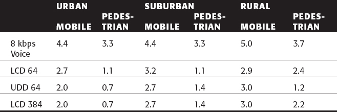
Coverage can actually improve for fast mobility users, since they become part of the channel averaging process. Fast power control works well for slow mobility users and provides useful gain particularly (as in the above example) where only minimal multipath diversity is available. Table 11.15 shows how important it is to optimize the power control algorithms in the handset and base station.

The process of power control is as follows:

Open-loop power control. This sets Tx power level based on the Rx power received by the mobile and compensates for path loss and slow fading.

Closed-loop power control. This responds to medium and fast fading and compensates for open-loop power control inaccuracies.

Outer-loop power control. This is implementation-specific, for example, the outer loop adjusts the closed loop control threshold in the base station to maintain the desired frame error rate. Closed-loop implementation at 1500 Hz uses 1/2 dB steps for urban and 1-dB steps for rural areas.

Table 11.15 Mobility Factors and Power Control Uplink E_b/N_o Requirements

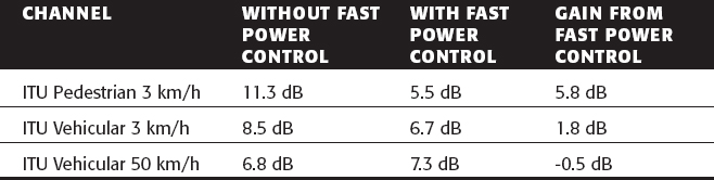
Power control needs to be optimized for certain operational conditions. Power control inaccuracies will substantially reduce capacity and coverage (by adding to noise rise). At higher speeds, fast power control is less effective in compensating channel fading. When carrying out a link budget for 3G, we therefore usually use an E_b/N_o figure for the service, channel type, and data rate assuming fast power control and then subtract a fast fading margin. The fast fading margin is approximately equivalent to the fast fading gain achieved by fast power control when the transmitter had no power limits. We normally expect the fast fading margin to be a few dB.

Uplink Budget Analysis

In previous cellular systems (1G and 2G) the link budget has been calculated on factors that are noninteractive and clearly definable (quantifiable) cell by cell. The differences between theoretical modeling results and practice have been mainly due to the inaccurate characterization of the propagation terrain and clutter factors. These problems still exist in 3G network planning but are added to by the interactive factors that we discussed earlier in this chapter. Link budget calculations will therefore have to take account of these additional factors.

We may consider some example assumptions:

Case 1

A 12.2 kbps voice service traveling at 120 kmph.

Assumptions:

• A 3 dB intracell interference rise (a cell loading of 50 percent).
• No intercell interference rise.
• Being voice, a soft handover is anticipated; hence, there will be some gain, let's assume 3 dB.
• A processing gain of 25 dB (10log3840/12.2).
• An E_b/N_o target of 5 dB.
• A fast fading margin of 0 dB—fast fading is ineffective at 120 kmph.

Case 2

144 kbps real-time data service traveling at 3 kmph.

Assumptions:

• Again, a 3 dB intracell interference rise (50 percent cell loading).
• A high transmit power is available as the mobile is away from the body. Hence, there are no body losses.
• An E_b/N_o target of 1.5 dB—as fast fading power control is effective at 3 kmph.
• Fast Fading Margin of 4 dB (the E_b/N_o target rises by 4 dB as the mobile moves to the cell edge).

It remains to be seen how true-to-life these considerations are (and become!).

Noise rise (as seen by the Node B) will be a function of the offered traffic measured as throughput. The amount, distribution, and burstiness of offered traffic all contribute to the achieved sensitivity in the Node B transceiver.

On the downlink, the capacity constraint may well be OVSF code-limited or orthogonality constraints (interrelated code domain effects). An orthogonality factor of 1 means the code streams are perfectly orthogonal. You will see orthogonality figures quoted in load factor calculations.

The downlink is more load-sensitive than the uplink. For example, one 10 W transmitter is shared amongst all users. On the uplink, each user has his or her own PA. The load limitation effectively limits downlink capacity. Increasing Node B power (downlink power) increases coverage and capacity but only at the cost of reducing the capacity and coverage available from adjacent cells.

Capacity calculations also need to take into account soft handover overheads. For a given number of cells, assumptions have to be made on uplink and downlink throughput and the number of users in soft handover.

Having established some capacity parameters, we need to establish the coverage available to users defined in terms of the service level being delivered to them. The coverage probability will be influenced by the mobility of the user—whether they are walking or driving or riding in a train.

Overall, the lessons learnt from 2G implementation 10 years ago were that early simulations based on (in GSM's case) relatively simple assumptions were overoptimistic. We might expect 3G simulations to be even wider off the mark, given the additional number of variables introduced into the simulation.

In practice, there will be a number of performance limitations in early 3G deployment that will make early link budget simulations hard to achieve.

Handset sensitivity generally improves as a technology matures partly because of device and design optimization and partly because volume product produces performance benefits (better control of component tolerance).

A similar pattern will probably emerge with IMT2000 handsets. Performance degrades if the air interface is required to do something it was not designed to do. This suggests that IMT2000 network performance will begin to settle down and provide good, consistent video and voice quality by 2005 to 2006.

A much more in-depth analysis of 3G system planning can be found in Radio Network Planning and Optimization for UMTS, published by Wiley and authored by Jaana Laiho, Achim Wacker, and Tomas Novosad, (ISBN 0-471-48653-1). Our thanks also to Mason Communications for their advice on system planning issues, some of which are referred to in the preceding text. Information on Mason Communications 3G system planning service is available at www.masoncom.com.

Long-Term Objectives in System Planning: Delivering Consistency

Radio bandwidth in a 3G network is more adaptive than radio bandwidth in a 2G network, which in turn is more adaptive than radio bandwidth in a 1G network. The OVSF code structure provides an elegant mechanism for balancing variable user data rates and allocating (code domain distributed) power. Pilot symbol based measurement reports provide a fast (1500 Hz) mechanism for measuring radio channel quality, which in turn provides the basis for accurate measurement reports, which in turn provides the basis for effective load balancing and admission control. Load balancing and admission control allow resources to be shared across the IP RAN network and radio layer in a more dynamically adaptable way than would be possible in existing legacy access networks (optimized for predominantly constant-rate offered traffic).

At the radio system level, load balancing between Node B transceivers helps to distribute offered noise. This helps improve average Node B sensitivity, which in turn helps improve coverage. Radio system capacity constraints are determined by the amount of RF power available both at the Node B and in the handset. The downlink can relatively quickly become code-limited because of the limited number of OVSF codes available. In larger cells, orthogonality can be a problem because of delay spread on the channel, and this can cause downlink performance degradation.

Coded channel streams (OVSF and long code streams) represent a phase argument that needs to be coherently demodulated, decorrelated, and combined by the receiver. Time, phase, or amplitude ambiguity on the radio channel will potentially impair performance (increase bit error rates).

Network performance is improved over time by optimizing radio layer and network layer performance parameters. There is a need for consistent quality, which in turn requires careful implementation of soft handover algorithms to avoid session discontinuity (or what used to be called high dropped call rates).

In the longer term (3 to 5 years), there is substantial gain potential in IMT2000, which will result in a more consistent radio channel. The challenge will be to deliver equivalent consistency into and through the IP RAN and IP core network to provide measurable and manageable end-to-end performance.

Wireless LAN Planning

In a number of countries, it is now permitted to provide public access services in the unlicensed industrial scientific medical bands. Bands of interest include the ISM band at 900 MHz (between 900 and 930 MHz) used for digital cordless phones in the United States, the ISM band at 2.4 GHz used for IEEE802 wireless LANs and Bluetooth, and the 5 GHz band used for wideband HIPERLANs (high-performance radio local area networks).

The availability of plug-in wireless LAN cards that include IEEE802 and Bluetooth have begun to focus attention on the need to integrate wide area wireless planning with in-building coverage planning.

One of the problems of planning in-building coverage is the unpredictability of in-building propagation, particularly at 2.4 GHz and 5 GHz (propagation unpredictability increases with frequency). Figure 11.18 shows a comparison between free space loss in an empty room and the loss in a room with cubicles partitioned off from one another. Signal levels received in the bare room are typically a few milliVolts. Signal levels received in the room with partitioning quickly attenuate down to a few microVolts. Losses are very dependent on the materials used in the partitioning. Fire-resistant silver foil, for example, will provide a high degree of shielding.

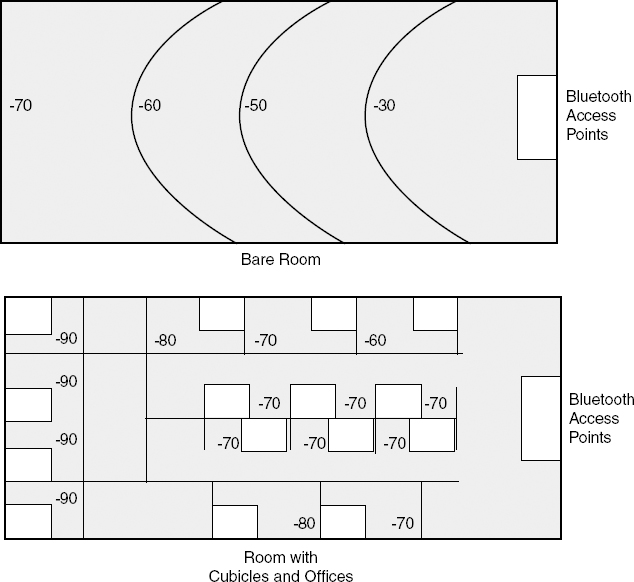
Figure 11.18 In-building received power.

In Figure 11.19 we show the minimum levels of attenuation normally experienced in a building, typically 6 or 7 dB floor to floor and 3 dB through a wall (without fire-resistant foil cladding). The attenuation through the exterior wall of the building will typically be 20 to 30 dB. This is good news and bad news. The good news is we probably do not want signals from inside the building to be visible outside the building and vice versa, both for security reasons and in order to deliver reasonable receive sensitivity.

However, present wireless LAN standards (IEEE802) include handover protocols that allow a user (theoretically) to move within a building (floor to floor) and into and out of buildings and still remain in continuous coverage. In practice, given the very substantial and rapid changes in signal level, it is very easy to drop a call under these conditions. It has also been proposed that wireless LAN to cellular handover should be supported. Again, in practice, this is hard to realize consistently because of the rapid fluctuation in received signal strength in the wireless LAN environment.

Figure 11.19 Minimum levels of attenuation in a building.

Designing a wireless LAN radio scheme is therefore a reasonably complex process and depends on having knowledge of the building configuration and building materials used. The process is not dissimilar to undertaking heat loss calculations/heat gain calculations from buildings where the sizing of the heating and cooling system is dependent on the building materials used, the size of windows, and whether windows are double or triple glazed. There are also many similarities with lighting design. Radio waves and light waves behave very similarly. In lighting calculations, we have to take into account the polar diagrams (also known as ISO candela diagrams) describing the light distribution available from the luminaire.

Unsurprisingly, this is very similar to looking at an RF antenna specification. Figure 11.20 shows a lighting product from Philips, and Figure 11.21 shows the related ISO candela diagram.

Figure 11.20 Example of a Philips lighting luminaire.

Figure 11.21 Isocandela flux intensity/polar intensity diagram for the luminaire in Figure 11.20.

It makes considerable sense to do a wireless coverage design at the same time as lighting design and heat loss calculations are being done for a building, since many of the inputs needed are common: the configuration and layout of the building and the materials used in the construction of the building. In lighting, we calculate lux intensity at various points in the room—the number of lumens on a desk, number of lumens reflecting off wall surfaces. In RF design, we calculate signal voltages available to RF receivers. The light output available from the luminaires (typically a few tens of Watts) is directly analogous to the RF power available from the wireless LAN transmitter (a few hundred milliWatts). Both lighting and RF design are directly affected by building geometry, user geometry (where people are in the building and what they are doing in the building), and the materials used in the building.

For further information on lighting design and integrated building services design, go to the Chartered Institute of Building Services Engineers Web site (www.cibse.org).

In designing for Bluetooth or IEEE802 RF wireless LAN coverage, we find, because of the wide variability of building geometry and building materials used, that range is not included in the specification, though there are guidelines offered based on the power output and receive sensitivity available. With Bluetooth, the guidelines suggest a range of 10 meters and 100-meter figures based on 0 dB and +20 dBm power output and assuming −70 dBm receiver sensitivity and −5 dBi antenna gain.

Although this may seem to be a reasonable assumption, in practice we have shown that there are typically attenuation effects of several tens of dBs to take into account. It is also in practice very difficult to deliver even moderate antenna efficiency because of space and size constraints and capacitive effects in handheld devices.

Cellular/Wireless LAN Integration

Ensuring consistent wireless LAN in building coverage is far from easy. Most installations are undertaken on the basis of rule of thumb estimates of how many transceivers are needed to provide continuous coverage across a given service area.

In many in-building environments, coverage from the cellular networks (either from outdoor microcells or indoor picocells) may well be more consistent than wireless LAN coverage. This makes handover protocols difficult to implement. Users will continuously be moved from wireless LAN to cellular coverage and back again. This in turn creates more discontinuity rather than less discontinuity in service provision. For these reasons, it is unlikely that wireless LAN/cellular technologies will be successfully integrated, at least for the immediately foreseeable future.

Distributed Antennas for In-Building Coverage

As we move from 2G to 3G technologies, base station form factor (at least temporarily) increases, the need to deliver more linearity increases base station Node B hardware footprint. At the same time, the minimum bandwidth available from a Node B transceiver is 5 MHz, compared to the minimum bandwidth of 200 kHz (an eight-slot, eight-channel single RF carrier mini GSM base station).

For in-building coverage we need small base stations and, often, not a lot of bandwidth. A base station in a small hotel foyer does not need 5 MHz of RF bandwidth. This makes distributed antennas quite attractive, certainly in the early stages of network deployment.

The idea of distributed antennas is to have a donor base station, say, in the basement of a large building. The RF signal is then distributed to a number of antennas mounted throughout the building. The problem with distributed antenna solutions is that losses in copper cable can be quite substantial.

One option is to use RF over fiber. The RF signal is converted to an optical signal using a linear laser and is then delivered down a fiber-optic cable. We cover RF over fiber in Chapter 13 (“Network Hardware Optimization”).

Summary

In this chapter we reviewed some of the important system design considerations implicit in implementing a 3G network with a 3G radio physical layer. We have said that the radio physical layer directly influences network performance, and we address this in more detail in future chapters.

We discussed some of the design and performance parameters of the Node B. We said that physical size (form factor) is driven by the ever-decreasing size and volume of 2G base stations and that a particular design challenge is to deliver the additional linearity needed in 3G hardware within a sufficiently compact, lightweight product footprint.

Node B hardware determines how much offered traffic can be supported and how the offered traffic will be accommodated in terms of cell sectorization. We introduced some of the radio layer enhancements that are available, such as downtilt antennas, and highlighted the differences between handset RF design and Node B design and some of the options for implementing Node B hardware (RF/IF and baseband processing). We emphasized that the RF performance of the Node B (code orthogonality on the downlink and receive sensitivity on the uplink) directly influences radio system planning.

In addition, we reviewed some of the lessons learned from system planning in 1G and 2G cellular networks and pointed out that initial coverage and capacity simulations are often overoptimistic. The additional number of variables in CDMA planning make it harder to pin down likely system performance.

We also reviewed some of the present simulations reviewed in the present planning literature and advised some caution in how the present figures should be interpreted. We pointed out that not only Node B RF performance but also handset RF performance is a major component of the RF link budget and that both Node B and handset RF performance increase as the network technology matures (particularly if market volume is achieved—the performance advantage of volume). A 1 dB improvement in Node B on handset sensitivity translates into a 10 percent decrease in network density

Finally, we reviewed indoor system planning and identified some of the significant attenuation effects introduced by building geometry and partitioning. We said that the rapid changes in signal level typical of in-building coverage presented particular challenges for managing handover in these environments. We suggested that there are commonalities between radio design or in-building coverage and lighting and heat loss/heat gain calculations.

In the longer term, a more integrated approach to radio planning and building design could well be beneficial.