CHAPTER 3

3G Handset Hardware

In the two previous chapters we identified that one of the principal design objectives in a cellular phone is to reduce component count, component complexity, and cost, and at the same time improve functionality. By functionality we mean dynamic range—that is, the range of operating conditions over which the phone will function—and the ability to support multiple simultaneous channels per user. We showed how GPRS could be implemented to provide a limited amount of bandwidth on demand and how GPRS could be configured to deliver, to a limited extent, a number of parallel channels, such as simultaneous voice and data. However, we also highlighted the additional cost and complexity that bandwidth on demand and multiple slots (multiple per user channel streams) introduced into a GSM or TDMA phone.

Getting Started

The general idea of a 3G air interface—IMT2000DS, TC, or MC—is to move the process of delivering sensitivity, selectivity, and stability from RF to baseband, saving on RF component count, RF component complexity, and cost, and increasing the channel selectivity available to individual users. You could, for example, support multiple channel streams by having multiple RF transceivers in a handset, but this would be expensive and tricky to implement, because too many RF frequencies would be mixing together in too small a space.

Our starting point is to review how the IMT2000DS air interface delivers sensitivity, selectivity, and stability, along with the associated handset hardware requirements. At radio frequencies, sensitivity is achieved by providing RF separation (duplex spacing) between send and receive, and selectivity is achieved by the spacing between RF channels—for example, 25 kHz (PMR), 30 kHz (AMPS or TDMA), 200 kHz (GSM), or 5 MHz (IMT2000DS).

At baseband, the same results can be achieved by using digital filtering; instead of RF channel spacing, we have coding distance, the measure of how separate—that is, how far apart—we can make our 0s and 1s. The greater the distance between a 0 and a 1, the more certain we are that the demodulated digital value is correct. An increase in coding distance equates to an increase in sensitivity.

Likewise, if we take two coded digital bit streams, the number of bit positions in which the two streams differ determines the difference or distance between the two code streams. The greater the distance between code streams, the better the selectivity The selectivity includes the separation of channels, the separation of users one from another, and the separation of users from any other interfering signal. The distance between the two codes (shown in Figure 3.1) is the number of bits in which the two codes differ (11!).

As code length increases, the opportunity for greater distance (that is, selectivity) increases. An increase in selectivity either requires an increase in RF bandwidth, or a lower bit rate.

Stability between two communicating devices can be achieved by locking two codes together (see Figure 3.2). This is used in TDMA systems to provide synchronization (the S burst in GSM is an example), with the base station providing a time reference to the handset.

In IMT2000DS, the code structure can be used to transfer a time reference from a Node B to a handset. In addition, a handset can obtain a time reference from a macro or micro site and transfer the reference to a simple, low-cost indoor picocell.

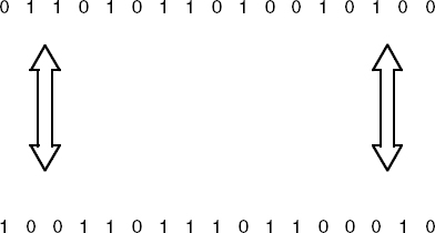
Figure 3.1 Coding distance–selectivity.

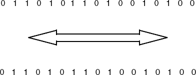
Figure 3.2 Code correlation–stability.

Code Properties

Direct-Sequence Spread Spectrum (DSSS) techniques create a wide RF bandwidth signal by multiplying the user data and control data with digital spreading codes. The wideband characteristics are used in 3G systems to help overcome propagation distortions.

As all users share the same frequency, it is necessary to create individual user discrimination by using unique code sequences. Whether a terminal has a dedicated communication link or is idle in a cell, it will require a number of defined parameters from the base station. For this reason, a number of parallel, or overlaying, codes are used (see Figure 3.3):

• Codes that are run at a higher clock, or chip, rate than the user or control data will expand the bandwidth as a function of the higher rate signal (code). These are spreading codes.
• Codes that run at the same rate as the spread signal are scrambling codes. They do not spread the bandwidth further.

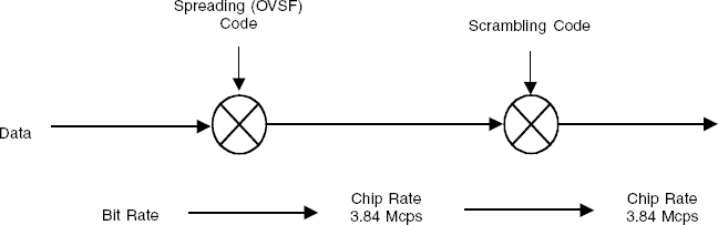
Figure 3.3 Spreading codes and scrambling codes.

The scrambling codes divide into long codes and short codes. Long codes are 38,400 chip length codes truncated to fit a 10-ms frame length. Short codes are 256 chips long and span one symbol period. On the downlink, long codes are used to separate cell energy of interest. Each Node B has a specific long code (one of 512). The handset uses the same long code to decorrelate the wanted signal (that is, the signal from the serving Node B). Scrambling codes are designed to have known and uniform limits to their mutual cross correlation; their distance from one another is known and should remain constant.

Code Properties—Orthogonality and Distance

Spreading codes are designed to be orthogonal. In a perfectly synchronous transmission, multiple codes co-sharing an RF channel will have no cross-code correlation; that is, they will exhibit perfect distance. The disadvantage with orthogonal codes is that they are limited in number for a given code length. Also, we need to find a family of codes that will support highly variable data rates while preserving most of their orthogonality. These are known as Orthogonal Variable Spreading Factor (OVSF) codes.

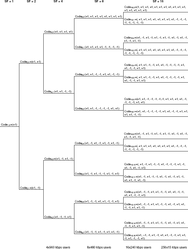
The variable is the number of symbols (also known as chips) used from the spreading code to cover the input data symbol. For a high bit rate (960 kbps) user, each data symbol will be multiplied with four spreading symbols, a 480 kbps user will have each data symbol multiplied with eight symbols, a 240 kbps user will have each data symbol multiplied with 16 symbols, and so on, ending up with a 15 kbps user having each data symbol multiplied with 256 symbols. In other words, as the input data/symbol rate increases, the chip cover decreases—and as a result, the spreading gain decreases.

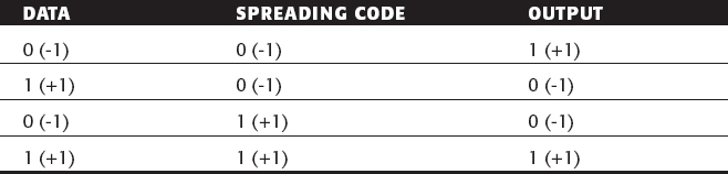
The input data (encoded voice, image, video, and channel coding) comes in as a 0 or a 1 and is described digitally as a +1 or as a −1. It is then multiplied with whatever the state of the spreading code is at any moment in time using the rule set shown in Tables 3.1 and 3.2.

Table 3.2 shows the OVSF code tree. We can use any of the codes from SF4 to SF256, though with a number of restrictions, which we will discuss in a moment.

Table 3.1 Exclusive NOR

Let's take a 480 kbps user with a chip cover of eight chips per data symbol, giving a spreading factor of 8 (SF 8).

User 1 is allocated Code 8.0

Input Data Symbol

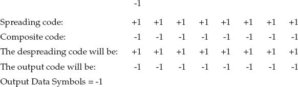
Effectively, we have qualified whether the data symbol is a +1 or −1 eight times and have hence increased its distance. In terms of voltage, our input data signal at −1 Volts will have become an output signal at −8 Volts when correlated over the eight symbol periods.

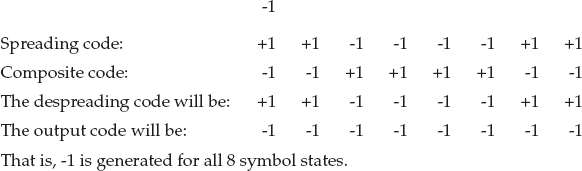
User 2 is allocated Code 8.3. The user's input symbol is also a −1.

Input Data Symbol

User 3 is allocated Code 8.5.

User 2's input data symbol will be exclusive NOR'd by User 3's despreading code as follows.

Input Data Symbol

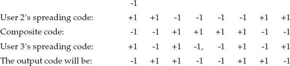
That is, the output is neither a +1 or a −1 but something in between. In other words, a distance has been created between User 2 and User 3 and the output stays in the noise floor.

Table 3.2 Spreading Codes

Code Capacity - Impact of the Code Tree and Non-Orthogonality

The rule set for the code tree is that if a user is, for example, allocated code 8.0, no users are allowed to occupy any of the codes to the right, since they would not be orthogonal.

A “fat” (480 kbps) user not only occupies Code 8.0 but effectively occupies 16.0 and 16.1, 32.0, 32.1, 32.2, 32.3, and so on down to 256.63. In other words, one “fat” user occupies 12.5% of all the available code bandwidth. You could theoretically have one high-bit-rate user on Code 8.0 and 192 “thin” (15 kbps) users on Code 256.65 through to Code 256.256:

• 1 × high-bit-rate user (Code 8)—Occupies 12.5% of the total code bandwidth.
• 192 × low-bit-rate users (Code 256)—Occupy all other codes 256.65 through 256.256.

In practice, the code tree can support rather less than the theoretical maximum, since orthogonality is compromised by other factors (essentially the impact of multipath delay on the code properties). Users can, however, be moved to left and right of the code tree, if necessary every 10 ms, delivering very flexible bandwidth on demand. These are very deterministic codes with a very simple and rigorously predefined structure. The useful property is the orthogonality, along with the ability to support variable data rates; the downside is the limited code bandwidth available.

From a hardware point of view, it is easy to move users left and right on the code tree, since it just involves moving the correlator to sample the spreading code at a faster or slower rate. On the downlink (Node B to handset), OVSF codes support individual users; that is, a single RF channel Node B (1 × 5 MHz) can theoretically support 4 high-bit-rate users (960 kbps), 256 × low-bit-rate (15 kbps) users, or any mix in between.

Alternatively, the Node B can support multiple (up to six) coded channels delivered to a single user—assuming the user's handset can decorrelate multiple code streams. Similarly, on the uplink, a handset can potentially deliver up to six simultaneously encoded code streams, each with a separate OVSF code. In practice, the peak-to-mean variation introduced by using multiple OVSF codes on the uplink is likely to prevent their use at least for the next three to five years, until such time as high degrees of power-efficient linearity are available in the handset PA.

We have said the following about the different code types:

Spreading codes. Run faster than the original input data. The particular class of code used for spreading is the OVSF code. It has very deterministic rules that help to preserve orthogonality in the presence of widely varying data rates.

Scrambling codes. Run at the same rate as the spread signal. They scramble but do not spread; the chip rate remains the same before and after scrambling. Scrambling codes are used to provide a second level of selectivity over and above the channel selectivity provided by the OVSF codes. They provide selectivity between different Node Bs on the downlink and selectivity between different users on the uplink. Scrambling codes, used in IMT2000DS, are Gold codes, a particular class of long code. While there is cross-correlation between long codes, the cross-correlation is uniform and bounded—rather like knowing that an adjacent RF channel creates a certain level of adjacent and co-channel interference. The outputs from the code-generating linear feedback register are generally configured, so that the code will exhibit good randomness to the extent that the code will appear noiselike but will follow a known rule set (needed for decorrelation). The codes are often described as Pseudo-Noise (PN) codes. When they are long, they have good distance properties.

Short codes. Short codes are good for fast correlation—for example, if we want to lock two codes together. We use short codes to help in code acquisition and synchronization.

In an IMT2000DS handset, user data is channel-coded, spread, then scrambled on the Tx side. Incoming data is descrambled then despread. The following section defines the hardware/software processes required to implement a typical W-CDMA receiver transmitter architecture. It is not a full description of the uplink and downlink protocol.

Common Channels

The downlink (Node B to handset) consists of a number of physical channels. One class (or group) of physical channels is the Common Control Physical CHannel (CCPCH). Information carried on the CCPCH is common to all handsets within a cell (or sector) and is used by handsets to synchronize to the network and assess the link characteristic when the mobile is in idle mode—that is, when it is not making a call. In dedicated connection mode—that is, making a call—the handset will still use part of the CCPCH information to assess cell handover and reselection processes, but will switch to using more specific handset information from the Dedicated CHannels (DCH) that are created in call setup.

The CCPCH consists of a Primary CCPCH (P-CCPCH) and a Secondary CCPCH (S-CCPCH). The P-CCPCH is time multiplexed together with the Synchronization CHannel (SCH) and carries the Broadcast CHannel (BCH).

Synchronization

The SCH consists of two channels: the primary SCH and the secondary SCH (see Figure 3.4). These are used to enable the mobile to synchronize to the network in order for the mobile to identify the base station-specific scrambling code.

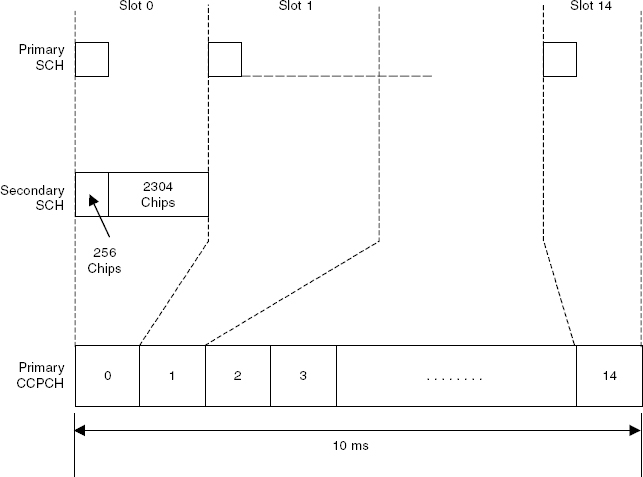
Figure 3.4 Primary and secondary SCH format.

The primary SCH is transmitted once every slot—that is, 15 times in a 10-ms frame. It is a 256-chip unmodulated spreading sequence that is common for the whole network—that is, identical in every cell. It is sent at the front of the 0.625-ms burst and defines the cell start boundary. Its primary function is to provide the handset with a timing reference for the secondary SCH. The secondary SCH, also 256 chips in length, is transmitted in every slot, but the code sequence, which is repeated for each frame, informs the handset of the long code (scrambling) group used by its current Node B.

As the primary SCH is the initial timing reference; in other words, it has no prior time indicator or marker, the receiver must be capable of detecting it at all times. For this reason, a matched filter is usually employed. The IF, produced by mixing the incoming RF with the LO, is applied to the matched filter. This is matching against the 256-bit primary SCH on the CCPCH. When a match is found, a pulse of output energy is produced. This pulse denotes the start of the slot and so is used to synchronize slot-recovery functions.

A 256 tap matched filter at a chip rate of 3.84 Mcps requires a billion calculations per second. However, as the filter coefficients are simply +1 −1 the implementation is reasonably straightforward. The remaining 2304 chips of the P-CCPCH slot form the BCH. As the BCH must be demodulated by all handsets, it is a fixed format. The channel rate is 30 kbps with a spreading ratio of 256, that is, producing a high process gain and consequently a robust signal. As the 256-bit SCH is taken out of the slot, the true bit rate is 27 kbps.

The Common Channels also include the Common PIlot CHannel (CPICH). This is an unmodulated channel that is sent as a continuous loop and is scrambled with the Node B primary scrambling code for the local cell. The CPICH assists the handset to estimate the channel propagation characteristic when it is in idle mode—that is, not in dedicated connection mode (making a call). In dedicated connection mode the handset will still use CPICH information (signal strength) to measure for cell handover and reselection. In connection mode the handset will use the pilot symbols carried in the dedicated channels to assess accurately the signal path characteristics (phase and amplitude) rather than the CPICH. The CPICH uses a spreading factor of 256—that is, high process gain for a robust signal.

Because the mobile only communicates to a Node B and not to any other handset, uplink common physical channels are not necessary. All uplink (handset to Node B) information—that is, data and reporting—is processed through dedicated channels.

Dedicated Channels

The second class of downlink physical channel is the Dedicated CHannel (DCH). The DCH is the mechanism through which specific user (handset) information (control + data) is conveyed. The DCH is used in both the downlink and uplink, although the channel format is different. The differences arise principally through the need to meet specific hardware objectives in the Node B and the handset—for example, conformance with EMC regulations, linearity/power trade-offs in the handset, handset complexity/processing power minimization, and so on.

The DCH is a time multiplex of the Dedicated Physical Control CHannel (DPCCH) and the Dedicated Physical Data CHannel (DPDCH), as shown in Figure 3.5. The DPCH is transmitted in time-multiplex with control information. The spreading factor of the physical channel (Pilot, TPC, and TFCI) may range from 512 to 4.

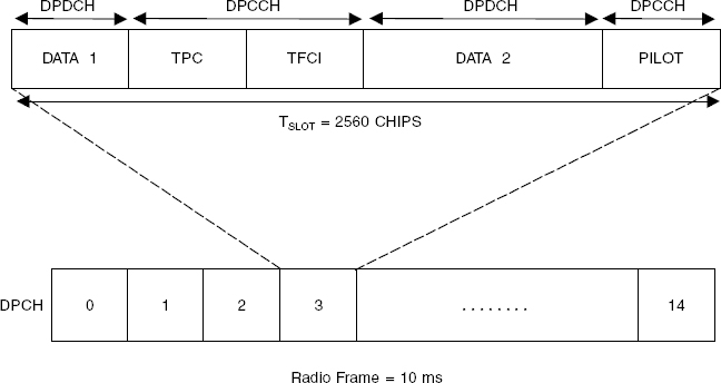
Figure 3.5 Dedicated channel frame structure.

The number of bits in each field may vary, that is:

• Pilot: 2 to 16
• TPC: 2 to 16
• TFCI: 0 to 16
• Data 1: 0 to 248
• Data 2: 2 to 1000

Certain bit/field combinations will require the use of DTX to maintain slot structure/timing.

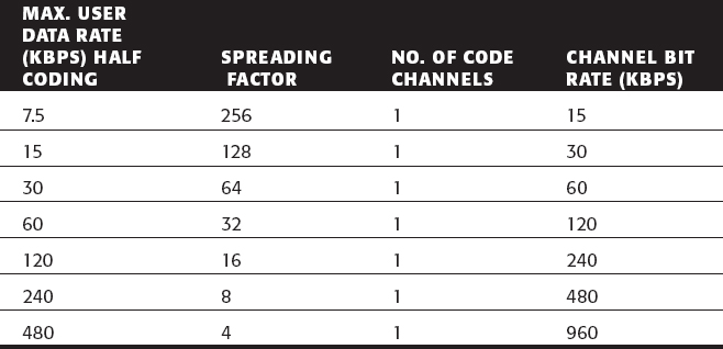
Table 3.3 shows spreading factors against user data rate. Low-bit-rate users have 24/25 dB of spreading gain, highest-bit-rate users 2/3 dB. From column 5, it is seen that the channel symbol rate can vary from 7.5 to 960 kbps. The dynamic range of the downlink channel is therefore 128:1, that is, 21 dB. The rate can change every 10 ms. In addition to spreading codes, scrambling codes are used on the downlink and uplink to deliver additional selectivity.

In the uplink, user data (DPDCH) is multiplexed together with control information (DPCCH) to form the uplink physical channel (DCH). Multiple DPDCH may be used with a single DPCCH. The DPCCH has a fixed spreading ratio of 256 and the DPDCH is variable (frame-by-frame), from 256 to 4 (see Table 3.4). Each DPCCH can contain four fields: Pilot, Transport Format Combination Indicator (TFCI), Transmission Power Control (TPC), and FeedBack Information (FBI). The FBI may consist of 0, 1, or 2 bits included when closed-loop transmit diversity is used in the downlink. The slot may or may not contain TFCI bits. The Pilot and TPC is always present, but the bit content compensates for the absence or presence of FBI or TFCI bits.

Table 3.3 Downlink Spreading Factors and Bit Rates

Table 3.4 Uplink DPDCH Rates

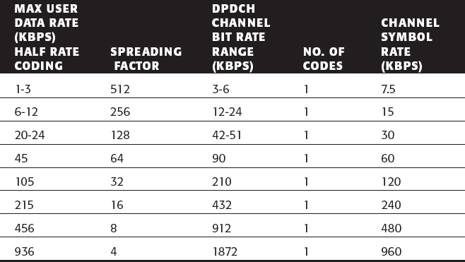
It is the variability of DPDCH (single to multiple channels) that define the dynamic range requirements of the transmitter PA, since multiple codes increase the peak-to-average ratio. From column 4, we see that the channel bit rate can vary from 15 to 960 kbps. The dynamic range of the channel is therefore 64:1—that is, 18 dB. The rate can change every 10 ms.

There are two types of physical channel on the uplink: dedicated physical data channel (DPDC) and dedicated physical control channel (DPCCH). The number of bits per uplink time slot can vary from 10 to 640 bits, corresponding with a user data rate of 15 kbps, to 0.96 Mbps. The user data rate includes channel coding, so the actual user bit rate may be 50 percent or even 25 percent of this rate.

Code Generation

Figure 3.6 shows how the OVSF codes and scrambling codes are applied on the transmit side and then used to decorrelate the signal energy of interest on the receive side, having been processed through a root raised cosine (RRC) filter. Channels are selected in the digital domain using a numerically controlled oscillator and a digital mixer.

Figure 3.7 shows steps in the uplink baseband generation. The DCCH is at a lower bit rate than the DTCH to ensure a robust control channel. Segmentation and matching is used to align the streams to a 10-ms frame structure. The composite signal is applied to the I stream component and the DPCCH carrying the pilot, power control, and TFCI bits with a spreading factor of 256 (providing good processing gain) applied to the Q stream.

The I and Q are coded with the scrambling code, and cross-coupled complex scrambling takes place to generate HPSK.

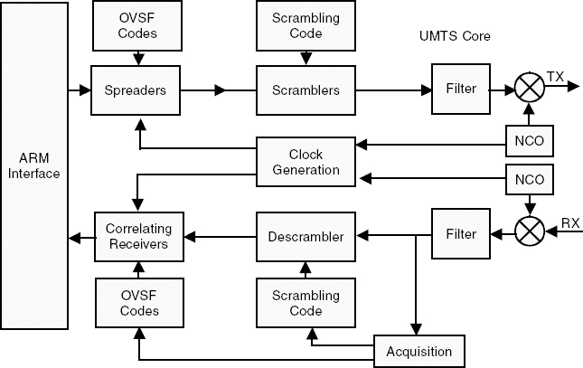
Figure 3.6 UMTS core for multimode 3G phones.

Hybrid phase shift keying, also known as orthogonal complex quadrature phase shift keying, allows handsets to transmit multiple channels at different amplitude levels while still maintaining acceptable peak-to-average power ratios. This process uses Walsh rotation, which effectively continuously rotates the modulation constellation to reduce the peak to average (PAR) of the signal prior to modulation.

Figure 3.7 is taken from Agilent's “Designing and Testing W-CDMA User Equipment” Application Note 1356. To summarize the processing so far, we have performed cyclic redundancy checking, forward error correction (FEC), interleaving, frame construction, rate matching, multiplexing of traffic and control channels, OVSF code generation and spreading, gain adjustment, spreading and multiplexing of the primary control channel, scrambling code generation, and HPSK modulation.

The feedback coefficients needed to implement the codes are specified in the 3GPP1 standards, as follows:

• Downlink:
  • 38,400 chips of 2¹⁸ Gold code
  • 512 different scrambling codes
  • Grouped for efficient cell search
• Uplink:
  • Long code: 38,400 chips of 225 Gold code
  • Short code: 256 chips of very large Kasami code

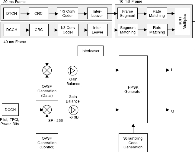
Figure 3.7 Uplink baseband generation.

An example hardware implementation might construct the function on a Xilinx Virtex device—it uses approximately 0.02 percent of the device, compared with the 25 percent required to implement an RRC/interpolator filter function.

Root Raised Cosine Filtering

We have now generated a source coded, 3.84 Mcps, I and Q streamed, HPSK formatted signal. Although the bandwidth occupancy of the signal is directly a function of the 3.84 Mcps spreading code, the signal will contain higher frequency components because of the digital composition of the signal. This may be verified by performing a Fourier analysis of the composite signal. However, we only have a 5 MHz bandwidth channel available to us, so the I and Q signals must be passed through filters to constrain the bandwidth. Although high-frequency components are removed from the signal, it is important that the consequent softening of the waveform has minimum impact on the channel BER. This objective can be met by using a class of filters referred to as Nyquist filters. A particular Nyquist filter is usually chosen, since it is easier to implement than other configurations: the raised cosine filter.

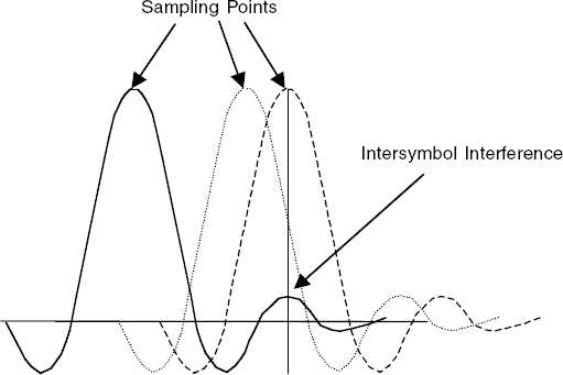
Figure 3.8 Filter pulse train showing ISI.

If an ideal pulse (hence, infinite bandwidth) representing a 1 is examined, it is seen that there is a large time window in which to test the amplitude of the pulse to check for its presence, that is, the total flat top. If the pulse is passed through a filter, it is seen that the optimum test time for the maximum amplitude is reduced to a very small time window. It is therefore important that each pulse (or bit) is able to develop its correct amplitude.

The frequency-limiting response of the filter has the effect of smearing or timestretching the energy of the pulse. When a train of pulses (bit stream) is passed through the filter, this ringing will cause an amount of energy from one pulse to still exist during the next. This carrying forward of energy is the cause of Inter-Symbol Interference (ISI), as shown in Figure 3.8.

The Nyquist filter has a response such that the ringing energy from one pulse passes through zero at the decision point of the next pulse and so has minimum effect on its level at this critical time (see Figure 3.9).

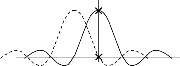
Figure 3.9 The Nyquist filter causes minimum ISI.

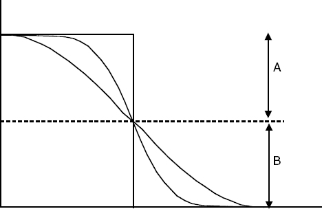
Figure 3.10 Symmetrical transition band.

The Nyquist filter exhibits a symmetrical transition band, as shown in Figure 3.10.

The cosine filter exhibits this characteristic and is referred to as a raised cosine filter, since its response is positioned above the base line.

It is the total communication channel that requires the Nyquist response (that is, the transmitter/receiver combination), and so half of the filter is implemented in the transmitter and the other half in the receiver. To create the correct overall response, a Root Raised Cosine (RRC) filter is used in each location as:

Modulation and Upconversion

Because the handset operates in a very power restrictive environment, all stages must be optimized not only for signal performance but also power efficiency. Following the RRC filtering, the signal must be modulated onto an IF and up-converted to the final transmission frequency. It is here the Node B and handset processes differ. The signal could continue to be processed digitally to generate a digitally sampled modulated IF to be converted in a fast DAC for analog up-conversion for final transmission. However, the power (DC) required for these stages prohibits this digital technique in the handset. (We will return to this process in Node B discussions.) Following the RRC filtering, the I and Q streams will be processed by matched DACs and the resulting analog signal applied to an analog vector modulator (see Figure 3.11).

A prime challenge in the design of a W-CDMA handset is to achieve the modulation and power amplification within a defined (low) power budget but with a minimum component count. This objective has been pursued aggressively in the design and implementation of later GSM handsets. Sufficient performance for a single-band (900 MHz) GSM phone was achieved in early-generation designs, but the inclusion of a second and third (and later fourth—800 MHz) band has driven the research toward minimum component architectures—especially filters. Chapter 2 introduced the offset loop transmitter architecture, which is successfully used for low-cost, low component count multiband GSM applications.

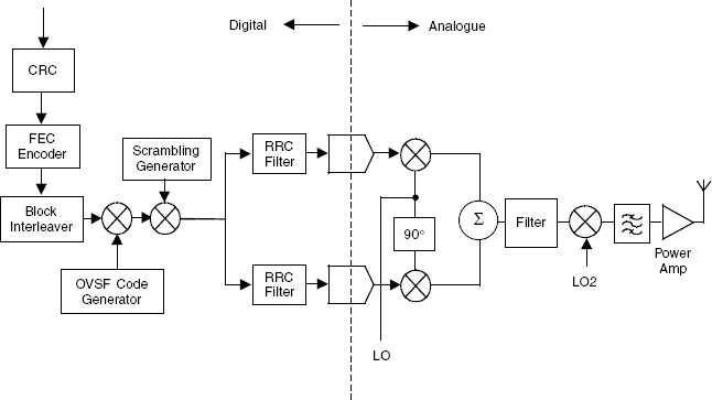
Figure 3.11 Typical digital/analog partitioning in a handset (analog vector modulator).

This architecture is very suitable for the GMSK modulation of GSM, as it has a constant amplitude envelope. The PLL configuration is only required to respond to the phase component of the carrier. The QPSK and HPSK modulation used in W-CDMA is non-constant envelope—that is, the modulated carrier contains both phase and amplitude components. Because the offset loop is unable to reproduce the amplitude components, it is unsuitable in its simple form. However, since it is particularly economic in components, there is considerable research directed toward using this technique for W-CDMA. To use the technique, the offset loop is used, with the amplitude components being removed by the loop function, but an amplitude modulator is used on the PA output to reproduce the amplitude components. This method of processing the carrier separately from its amplitude components is referred to as Envelope Elimination and Restoration (EER), as shown in Figure 3.12.

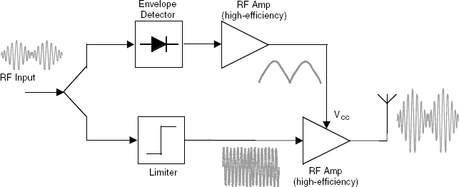
Figure 3.12 RF envelope elimination and restoration.

Other methods of producing sufficient PA linearity include adaptive predistortion and possibly the Cartesian loop technique although the latter is unlikely to stretch across the bandwidth/linearity requirement.

Power Control

All the decorrelation processes rely on coded channel streams being visible at the demodulator at similar received power levels (energy per bit) ideally within 1 dB of each other.

For every slot, the handset has to obtain channel estimates from the pilot bits, estimate the signal to interference ratio, and process the power control command (Transmission Power Control, or TPC), that is, power control takes place every 660 μs, or 1500 times per second. This is fast enough to track fast fading for users moving at up to 20 kmph. Every 10 ms, the handset decodes the Transport Format Combination Indicator (TFCI) which gives it the bit rate and channel decoding parameters for the next 10-ms frame. Data rates can change every 10 ms (dynamic rate matching) or at the establishment or teardown of a channel stream (static matching). The coding can change between 1/3 convolutional coding, 1/3 convolutional coding with additional block coding, /or turbo coding.

Power control hardware implementation will be similar to the detection methods outlined in Chapter 2 but the methods need to comprehend additional dynamic range and faster rates of change. The power control function also needs to be integrated with the linearization process.

The Receiver

As we have outlined in Chapter 2, there is a choice of superhet or zero/near-zero IF receiver architecture. If the superhet approach is chosen, it will certainly employ a sampled/digitized IF approach in order to provide the functional flexibility required. This approach enables us to realize a multimode—for example, GSM and W-CDMA—handset with a common hardware platform but with the modes differentiated by software. The following sections outline the functions that are required after sampling the IF in order to pass the signal to the RAKE receiver processes.

The Digital Receiver

The digital receiver consists of a digital local oscillator, digital mixer, and a decimating lowpass filter (see Figure 3.13). Digital samples from the ADC are split into two paths and applied to a pair of digital mixers. The mixers have digital local oscillator inputs of a quadrature signal—that is, sine and cosine—to enable the sampled IF to be mixed down to a lower frequency, usually positioned around 0 Hz (DC).

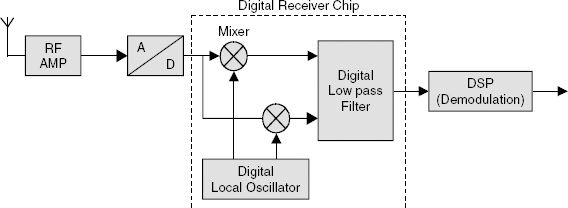
Figure 3.13 The digital receiver.

This process converts the digitized signal from a real to a complex signal, that is, a signal represented by its I and Q phase components. Because the signal is represented by two streams, the I and Q could be decimated by a factor of 2 at this point. However, because the down-shifted signal is usually processed for a single channel selection at this stage, the two decimation factors may be combined.

The LO waveform generation may be achieved by a number of different options—for example, by a Numerically Controlled Oscillator (NCO), also referred to as a Direct Digital Synthesizer (DDS)—if digital-to-analog converters are used on the I and Q outputs. In this process, a digital phase accumulator is used to address a lookup table (LUT), which is preprogrammed with sine/cosine samples. To maintain synchronization, the NCO is clocked by the ADC sampling/conversion clock.

The digital samples (sine/cosine) out of the local oscillator are generated at a sampling rate exactly equal to the ADC sample clock frequency fs. The sine frequency is programmable from DC to fs/2 and may be 32 bits. By the use of programmable phase advance, the resolution is usually sub-Hertz. The phase accumulator can maintain precise phase control, allowing phase-continuous switching. The mixer consists of two digital multipliers. Digital input samples from the ADC are mathematically multiplied by the digital sine and cosine samples from the LO. Because the data rates from the two mixer input sources match the ADC sampling rate (fs), the multipliers also operating at the same rate produce multiplied output product samples at fs. The I and Q outputs of the mixers are the frequency downshifted samples of the IF. The sample rate has not been changed; it is still the sample rate that was used to convert the IF.

The precision available in the mixing process allows processing down to DC (0 Hz). When the LO is tuned over its frequency range, any portion of the RF signal can be mixed down to DC; in other words, the wideband signal spectrums can be shifted around 0 Hz, left and right, by changing the LO frequency. The signal is now ready for filtering.

The decimating lowpass filter accepts input samples from the mixer output at the full ADC sampling frequency, fs. It uses digital signal processing to implement a finite impulse response (FIR) transfer function. The filter passes all signals from 0 Hz to a programmable cutoff frequency or bandwidth and rejects all signals higher than that cutoff frequency. The filter is a complex filter that processes both I and Q signals from the mixer. At the output either I or Q (complex) values or real values may be selected.

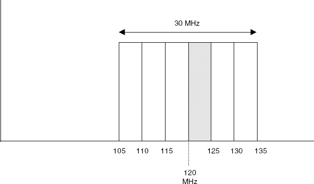
Figure 3.14 A 30 MHz signal digitized at an IF of 120 MHz.

An example will illustrate the processes involved in the digital receiver function (see Figure 3.14). The bandwidths—that is, number of channels sampled and digitized—in the sample may be outside a handset power budget; a practical design may convert only two or three channels. A 30 MHz (6 by 5 MHz W-CDMA RF channels) bandwidth signal has been sampled and digitized at an IF of 120 MHz.

It is required to process the channel occupying 120 to 125 MHz. When the LO is set to 122.5 MHz, the channel of interest is shifted down to a position around 0 Hz. When the decimating (lowpass) filter is set to cut off at 2.5 MHz, the channel of interest may be extracted (see Figure 3.15).

To set the filter bandwidth, you must set the decimation factor. The decimation factor is a function of both the output bandwidth and output sampling rate. The decimation factor, N, determines both the ratio between input and output sampling rates and the ratio between input and output bandwidths.

In the example in Figure 3.15, the input had a 30 MHz bandwidth input with a ±2.5 MHz bandwidth output. The decimation factor is therefore 30 MHz/2.5 MHz—that is, 12.

Digital receivers are divided into two classes, narrowband and wideband, defined by the range of decimation factors. Narrowband receivers range from 32 to 32,768 for real outputs, wideband receivers 1 to 32. When complex output samples are selected, the sampling rate is halved, as a pair of output samples are output with each sample clock. The downconverted, digitized, tuned around 0 Hz, filtered channel (bandwidth = 5 MHz) now exists as minimum sample rate I and Q bit streams. In this form it is now ready for baseband recovery and processing.

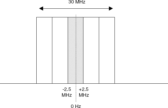
Figure 3.15 Selected channel shifted around 0 Hz.

The RAKE Receive Process

The signal, transmitted by the Node B or handset, will usually travel along several different paths to reach the receiver. This is due to the reflective and refractive surfaces that are encountered by the propagating signal. Because the multiple paths have different lengths, the transmitted signal has different arrival times (phases) at the receive antenna; in other words, the longer the path the greater the delay. 1G and 2G cellular technologies used techniques to select the strongest path for demodulation and processing. Spread spectrum technology, with its carrier time/phase recognition technique, is able to recover the signal energy from these multiple paths and combine it to yield a stronger signal.

Data signal energy is recovered in the spread spectrum process by multiplying synchronously, or despreading, the received RF with an exact copy of the code sequence that was used to spread it in the transmitter. Since there are several time-delayed versions of the received signal, the signal is applied simultaneously to a number of synchronous receivers, and if each receiver can be allocated to a separate multipath signal, there will be separate, despread, time-delayed recovered data streams. The data streams can be equalized in time (phase) and combined to produce a single output. This is the RAKE receiver.

To identify accurately the signal phase, the SCH is used. As already described, the received RF containing the SCH is applied to a 256-chip matched filter. This may be analog or sampled digitized IF. Multiple delayed versions of the same signal will produce multiple energy spikes at the output. Each spike defines the start of each delayed slot. (It is the same slot—the spikes define the multiple delays of the one slot.)

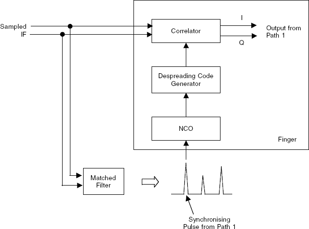
Figure 3.16 Matched filter for synchronizing I and Q.

Each spike is used as a timing reference for each RAKE receive correlator. The despreading code generator can be adjusted in phase by adjusting the phase of its clock. The clock is generated by an NCO—a digital waveform generator—that can be synchronized to a matched filter spike, that is, the SCH phase (see Figure 3.16).

Because the received signal has been processed with both scrambling and spreading codes, the code generators and correctors will generate scrambling codes to descramble (not despread) the signal and then OVSF codes to despread the signal. This process is done in parallel by multiple RAKE receivers or fingers. So now, each multipath echo has been despread but each finger correlator output is nonaligned in time. Part of the DPCCH, carried as part of the user-dedicated, or unique, channel is the pilot code. The known format of the pilot code bits enables the receiver to estimate the path characteristic—phase and attenuation. The result of this analysis is used to drive a phase rotator (one per RAKE finger) to rotate the phase of the signal of each finger to a common alignment. So, now we have multiple I and Q despread bit streams aligned in phase but at time-delayed intervals.

The last stage within each finger is to equalize the path delays, again using the matched filter information. Once the phase has been aligned, the delay has been aligned, and the various signal amplitudes have been weighted, the recovered energy of interest can be combined (see Figure 3.17).

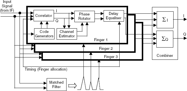
Figure 3.17 Combined signal energy of interest.

Path combining can be implemented in one of two ways. The simpler combining process uses equal gain; that is, the signal energy of each path is taken as received and, after phase and delay correction, is combined without any further weighting. Maximal ratio combining takes the received path signal amplitudes and weights the multipath signals by adding additional energy that is proportional to their recovered SNR. Although more complex, it does produce a consistently better composite signal quality. The complex amplitude estimate must be averaged over a sufficiently long period to obtain a mean value but not so long that the path (channel) characteristic changes over this time, that is, the coherence time.

Correlation

As we have described, optimum receive performance (BER) is dependent on the synchronous application of the despreading code to the received signal. Nonsynchronicity in the RAKE despreading process can be due to the random phase effects in the propagation path, accuracy and stability of the handset reference, and Doppler effects.

The process outlined in the previous section is capable of providing despreading alignment to an accuracy of one chip; however, this is not sufficient for low-BER, best demodulation. An accuracy of 1/8 chip or better is considered necessary for optimum performance.

As DSP/FPGA functions become increasingly power-efficient, greater use will be made of digital techniques (for example, digital filters) to address these requirements of fractional bit synchronization. Currently, methods employing delay lock loop (DLL) configurations are used to track and determine the received signal and despread code phase (see Figure 3.18). Code tracking can be achieved by the DLL tracking of PN signals. The principle of the DLL as an optimal device for tracking the delay difference between the acquired and the local sequence is very similar to that of the PLL that is used to track the frequency/phase of the carrier. Code tracking loops perform either coherently—that is, they have knowledge of the carrier phase—or noncoherently—that is, they do not have knowledge of the carrier phase.

Figure 3.18 The DLL.

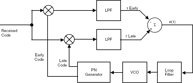
Two separate correlators are used, each with a separate code generator. One correlator is referred to as the early correlator and has a code reference waveform that is advanced in time (phase) by a fraction of a chip; the other correlator is the late correlator and is delayed but some fraction of a chip. The difference, or imbalance, between the correlations is indicative of the difference between the despread code timing and the received signal code.

The output signal e(τ) is the correction signal that is used to drive the PN generator clock (VCO or NCO—if digital). A third PN on time sequence can be generated from this process to be applied to an on-time correlator, or the correction could be applied to adjust the TCXO reference for synchronization.

A practical modification is usually applied to the DLL as described. The problem to be overcome is that of imbalance between the two correlators. Any imbalance will cause the loops to settle in an off-center condition—that is, not in synch. This is overcome by using the tau-dither early-late tracking loop.

The tau-dither loop uses one deciding correlator, one code generator, and a single loop, but it has the addition of a phase switch function to switch between an early and late phase—that is, advance and delay for the PN code tuning. In this way imbalance is avoided in the timing/synchronizing process, since all components are common to both early and late phases.

Receiver Link Budget Analysis

Because processing gain reduces as bit rate increases, receiver sensitivity must be determined across all possible data rates and for a required E_b/N_o (briefly, the ratio of energy per bit to the spectral noise density; we will discuss this further shortly). The calculation needs to comprehend the performance of the demodulator, which, in turn, is dependent on the level of modulation used. Other factors determining receiver sensitivity include the RF front end, mixer, IF stages, analog-to-digital converter, and baseband process (DSP). (See Figure 3.19.)

Let's look at a worked example in which we define receiver sensitivity. For example, let's determine receiver sensitivity at three data rates: 12.2 kbps, 64 kbps, and 1920 kbps at a BER of 1 in 10⁶.

The noise power is dimensioned by Boltzman's constant (k = 1.38 × 10⁻²³ J/K) and standardized to a temperature (T) of 290K (17° C). To make the value applicable to any calculation, it is normalized at a 1 Hz bandwidth. The value (k × T) is then multiplied up by the bandwidth (B) used.

The noise power value is then −174 dBm/Hz and is used as the floor reference in sensitivity/noise calculations. The receiver front end (RF + mixer) bandwidth is 60 MHz, in order to encompass IMT2000DS license options. The noise bandwidth of the front end is 10log₁₀(60MHz) = 77.8 dB. The receiver front noise floor reference is therefore −174 dBm +77.8 dB = −96.2 dBm. In the DSP, the CDMA signal is despread from 3.84 Mcps (occupying a 5 MHz bandwidth), to one of the three test data rates—12.2 kbps, 64 kbps, 1920 kbps—and can be further filtered to a bandwidth of approximately:

• Modulation bandwidth = Data rate × (1+ α)/log2(M) (where α = pulse-shaping filter roll-off and M = no of symbol states in modulation format)
• For IMT2000, α = 0.22 and M=4 (QPSK)

Thus, reduction in receiver noise due to despreading is as follows:

• = 10log₁₀(IF bandwidth/modulation BW)
• = 10log₁₀(5 MHz/7.5 kHz) = 28.2 dB for 12.2 kbps
• = 10log₁₀(5 MHz/39 kHz) = 21.1 dB for 64 kbps
• = 10log₁₀(5 MHz/1.25 MHz) = 6.0 dB for 1920 Mbps

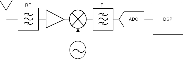
Figure 3.19 The digital IF receiver.

The effective receiver noise at each data detector due to input thermal noise is thus:

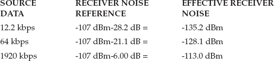
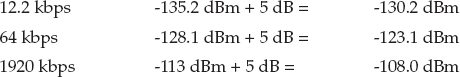
The real noise floor for a practical receiver will always be higher because of filter losses, LNA and mixer noise, synthesizer noise, and so on. In a well-designed receiver, 5 dB might be a reasonable figure. The practical effective noise floor of a receiver would then be

Using these figures as a basis, a calculation may be made of the receiver sensitivity. To determine receiver sensitivity, you must consider the minimum acceptable output quality from the radio. This minimum acceptable output quality (SINAD in analog systems, BER in digital systems) will be produced by a particular RF signal input level at the front end of the receiver. This signal input level defines the sensitivity of the receiver.

To achieve the target output quality (1 × 10⁻⁶ in this example), a specified signal (or carrier) quality is required at the input to the data demodulator. The quality of the demodulator signal is defined by its E_b/N_o value, where E_b is the energy per bit of information and N_o is the noise power density (that is, the thermal noise in 1 Hz of bandwidth). The demodulator output quality is expressed as BER, as shown in Figure 3.20. In the figure, a BER of 1 in 10⁶ requires an E_b/N_o of 10.5 dB.

Because receiver sensitivity is usually specified in terms of the input signal power (in dBm) for a given BER, and since we have determined the equivalent noise power in the data demodulator bandwidth, we need to express our E_b/N_o value as an S/N value. The S/N is obtained by applying both the data rate (R) and modulation bandwidth (B_M) to the signal, as follows:

• S/N = (E_b/N_o) × (R/B_M)
• For QPSK (M=4), B_M ~ R/2, thus:
• S/N = (E_b/No) × 2 = 14.5dB for BER = 1in 10⁶

Assuming a coding gain of 8 dB, we can now determine the required signal power (receive sensitivity) at the receiver to ensure we meet the (14.5–8) dB = 6.5 dB S/N target.

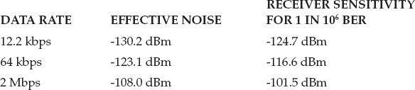
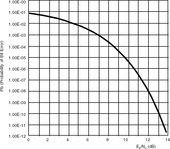
Figure 3.20 Bit error performance of a coherent QPSK system.

There is approximately 22 dB difference in sensitivity between 12.2 kbps speech and 2 Mbps data transfer, which will translate into a range reduction of approximately 50 percent, assuming r⁴ propagation, and a reduction in coverage area of some 75 percent!

IMT2000DS Carrier-to-Noise Ratio

In the 2G (GSM) system the quality of the signal through the receiver processing chain is determined primarily by the narrow bandwidth, that is, 200 kHz. This means that the SNR of the recovered baseband signal is determined by the 200 kHz IF filter positioned relatively early in the receive chain; little improvement in quality is available after this filter. Consequently the noise performance resolution and accuracy of the sampling ADC, which converts the CNR, must be sufficient to maintain this final quality SNR. When the W-CDMA process is considered, a different situation is seen. The sampled IF has a 5 MHz bandwidth and is very noisy—intentionally so. Because the CNR is poor, it does not require a high-resolution ADC at this point; large SNR improvement through the processing gain comes after the ADC. A fundamental product of the spreading/despreading process is the improvement in the CNR that can be obtained prior to demodulation and base band processing—the processing gain.

In direct-sequence spread spectrum the randomized (digital) data to be transmitted is multiplied together with a pseudorandom number (PN) binary sequence. The PN code is at a much higher rate than the modulating data, and so the resultant occupied bandwidth is defined by the PN code rate. The rate is referred to as the chip rate with the PN symbols as chips. The resultant wideband signal is transmitted and hence received by the spread spectrum receiver. The received wideband signal is multiplied by the same PN sequence that was used in the transmitter to spread it.

For the process to recover the original pre-spread signal energy it is necessary that the despreading multiplication be performed synchronously with the incoming signal. A key advantage of this process is the way in which interfering signals are handled. Since the despreading multiplication is synchronous with the transmitted signal, the modulation energy is recovered. However, the despreading multiplication is not synchronous with the interference, so spreads it out over the 5 MHz bandwidth. The result is that only a small portion of the interference energy (noise) appears in the recovered bandwidth.

Processing or despreading gain is the ratio of chip rate to the data rate. That is, if a 32-kbps data rate is spread with a chip rate of 3.84 Mcps, the processing gain is as follows:

The power of the processing gain can be seen by referring to the CNR required by the demodulation process. An E_b/N_o of 10.5 dB is required to demodulate a QPSK signal with a BER of 1 × 10⁻⁶. If a data rate of 960 kbps is transmitted with a chip cover of 3.84 Mcps, the processing gain is 6 dB. If a CNR of 10.5 dB is required at the demodulator and an improvement of 6.0 dB can be realized, the receiver will achieve the required performance with a CNR of just 4.5 dB in the RF/IF stages.

It must be considered at what point in the receiver chain this processing gain is obtained. The wideband IF is digitized and the despreading performed as a digital function after the ADC. Therefore, the ADC is working in a low-quality environment—4.5 dB CNR. The number of bits required to maintain compatibility with this signal is 6 or even 4 bits. The process gain is applied to the total spread signal content of the channel.

If the ADC dynamic range is to be restricted to 4 or 6 bits, consideration must be given to the incoming signal mean level dynamic range. Without some form of received signal dynamic range control, a variation of over 100 dB is typical; this would require at least an 18-bit ADC. To restrict the mean level variation within 4 or 6 bits, a system of variable-gain IF amplification (VGA) is used, controlled by the Received Signal Strength Indication (RSSI).

Prior to the change to 3.84 Mcps, the chip rate was at 4.096 Mcps, which when applied to a filter with a roll-off factor of 1.22 gave a bandwidth of 5 MHz. Maintaining the filter at 1.22 will give an improved adjacent channel performance. The process gain is applied to the total spread signal content of the channel. For example, a 9.6-kbps speech signal is channel-coded up to a rate of 32 kbps. The process gain is therefore 10 log(3.84/0.032) = 20.8 dB, not 10log(3.84/0.0096) = 26 dB, as may have been anticipated (or hoped for).

Receiver Front-End Processing

In a digitally sampled IF superhet receiver, the front end (filter, LNA, mixer, and IF filter/pre-amplifier) prepares the signal for analog to digital conversion. The parameters specifying the front end need to be evaluated in conjunction with the chosen ADC. An IMT2000DS example will be used to show an approach to this process.

The receiver performance will be noise-limited with no in-band spurs that would otherwise limit performance. This is reasonable because the LO and IF can be chosen such that unwanted products do not fall in-band. Spurs that may be generated within the ADC are usually not a problem, because they can be eliminated by adding dither or by carefully choosing the signal placement.

The superhet receiver will have a front-end bandwidth of 60 MHz, to encompass the total spectrum allocation and a digitizing, demodulation, and processing bandwidth of 5 MHz, as defined for W-CDMA. To meet the stringent power consumption and minimum components requirement, the receiver will be realized as a single conversion superhet (see Figure 3.21).

The first step is a gain and noise budget analysis to X——X. The dB figures are converted to ratios:

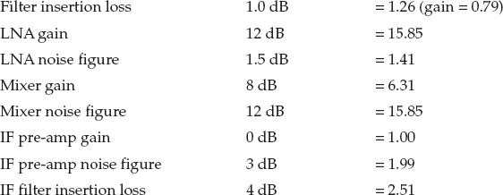
Using the Friis equation, the composite noise factor (linear) can be calculated:

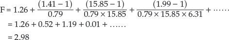
The noise figure is therefore:

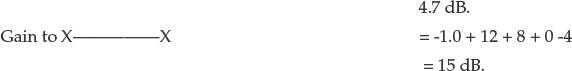
The front end has a noise figure of 4.7 dB and a conversion gain of 15 dB. An evaluation is made of the noise power reaching X——X (considered in a 5 MHz bandwidth).

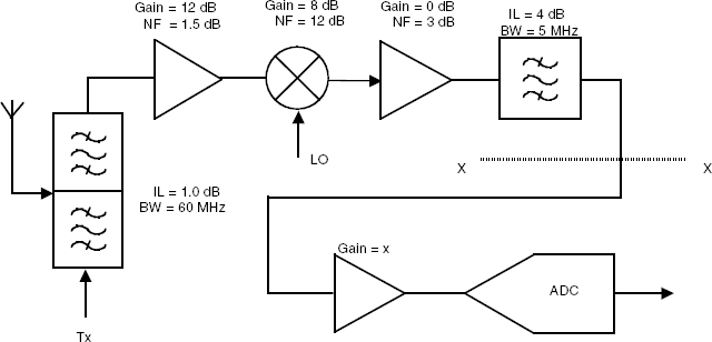
Figure 3.21 W-CDMA superhet receiver.

Noise power in a 5 MHz bandwidth, above the noise floor, is as follows:

= −174 dB/Hz + 10 log 5 MHz

= −174 + 67

= −107 dBm

The RF/IF noise power (in a 5 MHz bandwidth) to be presented to the ADC is as follows:

= −107 + 15 + 4.7

= −87.3 dBm

If the receiver input signal is −114.2 dBm (for a 64 kbps data stream with 10⁻³ BER), then the signal level at X——X is as follows:

= −114.2 dBm + 15

= −99.2 dBm

Therefore, the CNR in the analog IF is as follows:

= −87.3 (−)—92.2

= −11.9 dB.

It is necessary to calculate the minimum quantization level of the ADC. An 8-bit ADC with a full-scale input of 1 V pk-pk will be chosen:

1 bit level = 1 V/2^N

where N = the number of bits:

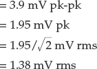
The output of the stage preceding the ADC will be assumed to have a 50-ohm impedance. It is necessary to normalize the ADC minimum quantization level to 50 ohms:

The noise power threshold presented to the ADC, however, is −87.3 dBm. For the ADC to see the minimum signal, the input must be raised to −44.2 dBm. This can be achieved by a gain stage, or stages, before the ADC, where gain

= −87.3 (−)−44.2

= 43.1 dB

An alternative process is to add out-of-band noise—to dither the ADC across the minimum quantization threshold. This minimizes the impact on the CNR of the signal but may not be necessary given the noisy nature of a W-CDMA signal.

Received Signal Strength

The received signal strength for both mobile handsets and fixed base stations in a cellular network is widely varying and unpredictable, because of the variable nature of the propagation path. Since the handset and Node B receiver front end must be extremely linear to prevent intermodulation occurring, the variation of signal strength persists through the RF stages (filter, LNA, mixer) and into the IF section.

A customary approach to IF and baseband processing in the superhet receiver is to sample and digitize the modulated IF. The IF + modulation must be sampled at a rate and a quality that maintains the integrity of the highest-frequency component—that is, IF + (modulation bandwidth/2). The digitization may be performed at a similar rate (oversampling) or at a lesser rate calculated from the modulation bandwidth (bandwidth or undersampling). Either digitization method must fulfill the Nyquist criteria based on the chosen process (oversampling or bandwidth sampling).

From an analysis of the sampling method, modulation bandwidth, required CNR, and analog-to-digital converter linearity, the necessary number of ADC bits (resolution) can be calculated. The number of bits and linearity of the ADC will give the spurious free dynamic range (SFDR) of the conversion process.

For TDMA handset requirements, the resolution will be in the order of 8 to 10 bits. For IMT2000DS/MC, 4 to 6 bits may be acceptable. Typical received signal strength variation can be in excess of 100 dB. This equates to a digital dynamic range of 16 or 18 bits. The implementation option is therefore to use a 16 to 18 bit ADC, or to reduce the signal strength variation presented to the ADC to fit within the chosen number of ADC bits.

A typical approach to signal dynamic range reduction is to alter the RF or IF gain, or both, inversely to the signal strength prior to analog-to-digital conversion. The process of gain control is referred to as AGC (automatic gain control) and uses variable-gain amplifiers controlled by the RSSI.

RSSI response time must be fast enough to track the rate of change of mean signal strength—to prevent momentary overload of subsequent circuits—but not so fast that it tracks the modulation envelope variation, removing or reducing modulation depth. The RSSI function may be performed by a detector working directly on the IF or by baseband processing that can average or integrate the signal over a period of time.

Simple diode detectors have been previously used to measure received signal strength. They suffer from limited dynamic range (20/25 dB), poor temperature stability, and inaccuracy. The preferred method is to use a multistage, wide-range logarithmic amplifier. The frequency response can be hundreds of MHz with a dynamic range typically of 80/90 dB.

The variable amplifiers require adequate frequency response, sufficient dynamic range control (typically 60 dB+), and low distortion. Additionally, the speed of response must track rate of mean signal level change. It is a bonus if they can directly drive the ADC input, that is, with a minimum of external buffering.

The concept of dynamic range control has a limited application in base station receivers, as weak and strong signals may be required simultaneously. If the gain was reduced by a strong signal, a weak signal may be depressed below the detection threshold. A wider dynamic range ADC must be used.

IMT2000TC

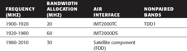
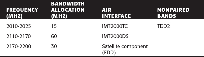
In Chapter 1 we identified that some operators were being allocated 2 × 10 MHz paired channel allocations for IMT2000 and 1 × 5 MHz nonpaired channel (see Table 3.5). There are two nonpaired bands:

• TDD1 covers 4 × 5 MHz channels between 1900 and 1920 MHz.
• TDD2 covers 3 × 5MHz channels between 2010 and 2025 MHz.

Table 3.5 Band Allocations Including Nonpaired Bands (TDD1 and TDD2)

Because the channel is not duplex spaced (the same RF channel is used for downlink and uplink), the channel is reciprocal. It is therefore theoretically possible to use the RAKE filter in the handset as a predistortion device. The benefit is that this allows the implementation of a relatively simple (i.e., RAKE-less) picocell base station.

The frame and code structure are slightly different to IMT2000DS. The 15-slot 10-ms frame is retained, but each of slots can support a separate user or channel. Each user or channel slot can then be subdivided into 16 OVSF spreading codes. The spreading factors are from 1 to 16. (Spreading factor 1 does not spread!)

The combination of time-division duplexing, time-division multiplexing, and a code multiplex provides additional flexibility in terms of bandwidth on demand, including the ability to support highly asymmetric channels. The duty cycle can also be actively reduced (a 1/15 duty cycle represents a 12 dB reduction in power). A mid-amble replaces the pilot tone and provides the basis for coherent detection. We revisit IMT2000TC access protocols in Part III of this book, “3G Network Hardware.”

GPS

In addition to producing a dual-mode IMT2000DS/IMT2000 TC handset, the designer may be required to integrate positioning capability. There are at least eight technology options for providing location information: cell ID (with accuracy dependent on network density), time difference of arrival, angle of arrival, enhanced observed time difference (handset-based measurement), two satellite options (GPS and GLONASS, or Global Navigation Satellite System), a possible third satellite option (Galileo), and assisted GPS (network measurements plus GPS).

GPS receives a signal from any of the 24 satellites (typically 3 or 4) providing global coverage either at 1.5 GHz or at 1.5 GHz and 1.1 GHz, for higher accuracy. The RF carrier carries a 50 bps navigational message from each satellite giving the current time (every 6 seconds), where the satellite is in its orbit (every 30 seconds) and information on all satellite positions (every 12.5 minutes). The 50 bps data stream is spread with a 1.023 Mcps PN code.

The huge spreading ratio (1,023,000,000 bps divided by 50) means that the GPS receiver can work with a very low received signal level—typically 70 nV into 50 ohms, compared to a handset receiving at 1 μV. In other words, the GPS signal is 143 times smaller. The received signal energy is typically −130 dBm. The noise floor of the receiver is between −112 dBm and −114 dBm (i.e., the received signal is 16 to 18 dB below the noise floor).

Although the GPS signal is at a much lower level, GPS and IMT2000DS do share a similar signal-to-noise ratio, which means that similar receiver processing can be used to recover both signals. The practical problem tends to be the low signal amplitudes and high gains needed with GPS, which can result in the GPS receiver becoming desensitized by the locally generated IMT2000 signal. The solution is to provide very good shielding, to be very careful on where the GPS antenna is placed in relation to the IMT2000 antenna, or to not receive when the handset is transmitting.

If the GPS receiver is only allowed to work when the cellular handset is idle, significant attention has to be paid to reducing acquisition time.

An additional option is to use assisted GPS (A-GPS). In A-GPS, because the network knows where the handset is physically and knows the time, it can tell the handset which PN codes to use (which correlate with the satellites known to be visible overhead). This reduces acquisition time to 100 ms or less for the three satellites needed for latitude, longitude, and altitude, or the four satellites needed for longitude, latitude, and altitude.

Bluetooth/IEEE802 Integration

Suppose that, after you've designed an IMT2000DS phone that can also support IMT2000TC and GSM 800, 900, 1800, the marketing team reminds you that you have to include a Bluetooth transceiver. Bluetooth is a low-power transceiver (maximum 100 mW) that uses simple FM modulation/demodulation and frequency hopping at 1600 hops per second over 79 × 1 MHz hop frequency between 2.402 and 2.480 GHz (the Industrial Scientific Medical, or ISM, band). Transmit power can be reduced from 100 mW (+20 dBm) to 0 dBm (1.00 mW) to −30 dBm (1μW) for very local access, such as phone-to-ear, applications.

Early implementations of Bluetooth were typically two-chip, which provided better sensitivity at a higher cost; however, present trends are to integrate RF and baseband into one chip, using CMOS for the integrated device, which is low-cost but noisy. The design challenge is to maintain receive sensitivity both in terms of device noise and interference from other functions within the phone.

Supporting IEEE 802 wireless LAN connectivity is also possible, though not necessarily easy or advisable. The IEEE 802 standard supports frequency hopping and direct-sequence transceivers in the same frequency allocation as Bluetooth. Direct sequence provides more processing gain and coherent demodulation (with 3 dB of sensitivity) compared to the frequency hopping option, but it needs a linear IQ modulator, automatic frequency control for I/Q spin control, and a linear power amplifier.

Infrared

Infrared provides an additional alternative option for local access wireless connectivity. The infrared port on many handsets is used for calibration as the handset moves down the production line, so it has paid for itself before it leaves the factory. Costs are also low, typically less than $1.50.

Infrared standards are evolving. The ETSI/ARIB IRDA AIR standard (area infrared) supports 120° beamwidths, 4 Mbps data rates over 4 meters, and 260 kbps over 8 meters. This compares to a maximum 432.6 kbps of symmetric bandwidth available for Bluetooth.

IEEE 802 also supports an infrared platform in the 850- to 950-nanometer band, giving up to 2 W peak power, 4- or 16-level pulse modulation, and a throughput of 2 Mbps. Higher bit rate RF options are available in the 5 GHz ISM band, but at present these are not included in mainstream 3G cellular handset specifications.

Radio Bandwidth Quality/Frequency Domain Issues

We have just described how code domain processing is used in IMT2000DS to improve radio bandwidth quality. Within the physical layer, we also need to comprehend frequency domain and time domain processing. If we wished to be very specific, we would include source coding gain (using processor bandwidth to improve the quality of the source coded content), coherence bandwidth gain (frequency domain processing), spreading gain (code domain processing), and processing gain (time domain processing, that is, block codes and convolutional encoders/decoders).

Let's first review some of the frequency domain processing issues (see Table 3.6). We said that the IMT2000 spectrum is tidily allocated in two 60 MHz paired bands between 1920-80 and 2110 and 2170 MHz with a 190 MHz duplex spacing. In practice, the allocations are not particularly tidy and vary in minor but significant ways country by country.

Table 3.6 IMT2000 Frequency Plan

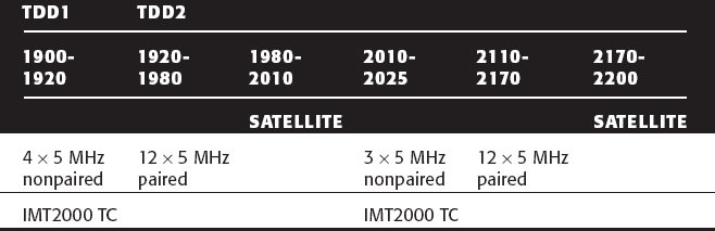
Figure 3.22 shows how spectrum was allocated/auctioned in the United Kingdom. It is not untypical of any country in which the spectrum is divided up between five operators, as follows:

• License A (Hutchison) has 14.6 MHz (3 × 5 MHz less a guard band) paired band allocation.
• License B (Vodafone) has 14.8 MHz (3 × 5 MHz less a guard band) paired band allocation.
• License C (BT3G) has 10 MHz (2 × 5 MHz allocation in the paired band) and 5 MHz at 1910 MHz in the TDD1 nonpaired band.
• License D (One2One) has 10 MHz (2 × 5 MHz allocation in the paired band) and 5 MHz at 1900 MHz in the TDD1 nonpaired band.
• License E (Orange) has 10 MHz (2 × 5 MHz in the paired band) and 5 MHz at 1905 MHz in the TDD1 nonpaired band.

The German allocation is different in that 10 MHz of paired bandwidth is allocated to six operators (6 × 10 MHz = 60 MHz), then all four of the TDD1 channels are allocated (1900 to 1920 MHz), along with one of the TDD2 channels (see Figure 3.23).

3GPP1 also specifies an optional duplex split of 134.8 and 245.2 MHz to support possible future pairing of the TDD1 and TDD2 bands. Although this is unlikely to be implemented, the flexible duplex is supported in a number of handset and Node B architectures.

The fact that 5 MHz channels are allocated differently in different countries means that operators must be prepared to do code planning and avoid the use of codes that cause adjacent channel interference to either other operators in the same country or other operators in immediately adjacent countries. It is therefore important to explore the interrelationship between particular combinations of spreading codes and adjacent channel performance.

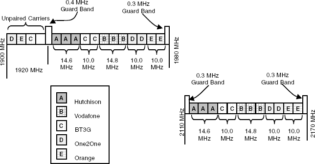
Figure 3.22 Countries with five operators–for example, United Kingdom.

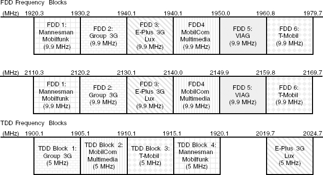
Figure 3.23 Countries with six operators–for example, Germany.

The three measurements used are as follows:

• ACLR (Adjacent Channel Leakage Ratio), formerly Adjacent Channel Power Ratio
• ACS (Adjacent Channel Selectivity)
• ACIR (Adjacent Channel Interference Ratio), formerly Adjacent Channel Protection Ratio.

OVSF code properties also determine peak-to-average ratios (PAR), in effect the AM components produced as a result of the composite code structure. PAR in turn determines RF PA (RF Power Amplifier) linearity requirements, which in turn determine adjacent channel performance. In other words, peak-to-average power ratios are a consequence of the properties of the offered traffic—the instantaneous bit rate and number of codes needed to support the per user multiplex.

We find ourselves in an interactive loop: We can only determine frequency domain performance if we know what the power spectral density of our modulated signal will be, and we only know this if we can identify statistically our likely offered traffic mix.

Out-of-channel performance is qualified using complementary cumulative distribution functions—the peak-to-average level in dB versus the statistical probability that this level or greater is attained. We use CCDF to calculate the required performance of particular system components and, for example, the RF PA.

ACLR is the ratio of transmitted power to the power measured after a receiver filter in the adjacent RF channel. It is used to qualify transmitter performance. ACS is the ratio of receiver filter attenuation on the assigned channel frequency to the receiver filter attenuation on the adjacent channel frequency and is used to qualify receiver performance. When we come to qualify system performance, we use ACIR—the adjacent channel interference ratio. ACIR is derived as follows:

(We review system performance in Chapter 11 on network hardware.)

As a handset designer, relaxing ACLR, in order to improve PA efficiency, would be useful. From a system design perspective, tightening ACLR would be helpful, in order to increase adjacent channel performance. ACLR is in effect a measure of the impact of nonlinearity in the handset and Node B RF PA.

We can establish a conformance specification for ACLR for the handset but need to qualify this by deciding what the PAR (ratio of the peak envelope power to the average envelope power of the signal) will be. We can minimize PAR, for example, by scrambling QPSK on the uplink (HPSK) or avoiding multicodes. Either way, we need to ensure the PA can handle the PAR while still maintaining good ACL performance. We can qualify this design trade-off using the complementary cumulative distribution function.

A typical IMT2000DS handset ACLR specification would be as follows:

• 33 dBc or −50 dBm at 5 MHz offset
• 43 dBc or −40 dBm at 10 MHz offset

Radio Bandwidth Quality/Time Domain Issues

We mentioned channel coding briefly in Chapter 1. 3G cellular handsets and Node Bs use many of the same channel coding techniques as 2G cellular—for example, block coding and convolutional coding. We showed how additional coding gain could be achieved by increasing the constraint length of a convolutional decoder. This was demonstrated to yield typically a 1/2 dB or 1 dB gain, but at the expense of additional decoder complexity, including processor overhead and processor delay.

In GPRS, adaptive coding has been, and is being, implemented to respond to changes in signal strength as a user moves away from a base station. This has a rather unfortunate side effect of increasing a user's file size as he or she moves away from the base station. At time of writing only CS1 and CS2 are implemented.

We also described interleaving in Chapter 1 and pointed out that increasing the interleaving depth increased the coding gain but at the cost of additional fixed delay (between 10 and 80 ms). Interleaving has the benefit of distributing bit errors, which means that convolutional decoders produce cleaner coding gain and do not cause error extension. If interleaving delay is allowable, additional coding gain can be achieved by using turbo coding.

IMT2000 Channel Coding

In IMT2000 the coding can be adaptive depending on the bit error rate required. The coding can be one of the following:

• Rate 1/3 convolutional coding for low-delay services with moderate error rate requirements (1 in 10³)
• 1/3 convolutional coding and outer Reed-Solomon coding plus interleaving for a 1 in 10⁶ bit error rate

In IMT2000 parallel code concatenation, turbo coding is used. Turbo codes have been applied to digital transmission technology since 1993 and show a practical tradeoff between performance and complexity. Parallel code concatenation uses two constituent encoders in parallel configuration with a turbo code internal interleaver. The turbo coder has a 1/3 coding rate. The final action is enhancement of E_b/N_o by employing puncturing.

Turbo coders are sometimes known as maximum a posteriori decoders. They use prior (a priori) and post (a posteriori) estimates of a code word to confer distance.

Reed-Solomon, Viterbi, and Turbo Codes in IMT2000

For IMT2000, Reed-Solomon block codes, Viterbi convolutional codes, and turbo codes are employed. The combination of Reed-Solomon and Viterbi coding can give an improvement in S/N for a given BER of 6 to 7 dB. Turbo coding used on the 1 × 10-6 traffic adds a further 1.5- to 3 dB improvement. Total coding gain is ∼ 8 dB.

The benefit of coding gain is only obtained above the coding threshold, that is, when a reasonable amount of E_b/N_o is available (rather analogous to wideband FM demodulator gain—the capture effect). Turbo coding needs 300 bits per TTI (Transmission Time Interval) to make turbo coding more effective than convolutional coding. This means turbo coding only works effectively when it is fed with a large block size (anything up to 5114 bits blocks). This adds to the delay budget and means that turbo coding is nonoptimum for delay-sensitive services.

Future Modulation Options

Present modulation schemes used in IMT2000DS are QPSK, along with HPSK on the uplink. 8 PSK EDGE modulation also needs to be supported. In 1xEV, 16-level QAM is also supported.

As the modulation trellis becomes more complex—that is, the phase and amplitude states become closer together and symbol time recovery becomes more critical—-it becomes worthwhile to consider trellis coding. In trellis coding, where modulation states are close together, the data is coded for maximal distance; when the data is far apart, they are coded for minimal distance. Trellis coding is used in certain satellite access and fixed access networks.

Characterizing Delay Spread

Delay spread is caused by multipath on the radio channel—that is, different multiple path lengths between transmitter and receiver. Radio waves reflecting off buildings will also change in phase and amplitude. Radio waves travel at 300,000 kmps. This means that in 1 ms they will have traveled 300 km, in 250 μ they will have traveled 75 km, and in 25 μs they will have traveled 7.5 km.

A 1 km flight time is equivalent to an elapsed time of 3.33 2 μ, and a 100 m flight time is equivalent to an elapsed time of 0.33 μs. In other words, delay spread is a function of flight time. Radio waves take approximately 3.33 2 μ to travel 1 km. A 100-m difference between two path lengths is equivalent to a delay difference of 0.33 μs. Chip duration in IMT2000 DS is 0.26 μs. Therefore, multipaths of >70 m are resolvable; multipaths of <70 m are not. If all the energy of each chip in a user's chip sequence falls within one chip period, you do not need a RAKE receiver.

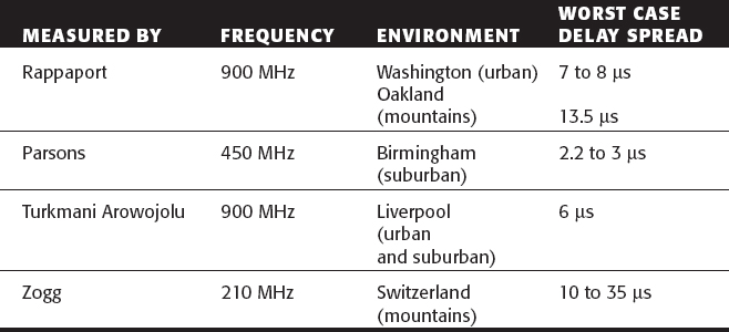
Delay spreads increase as you go from dense urban-to-urban to suburban and are largest, as you would expect, in mountainous areas (termed the “Swiss mountain effect”). Table 3.7 shows typical measured delay spreads. In GSM, the GSM equalizer specification defines that the equalizer should be capable of correcting a 4-bit shift on the channel (that is, a 16 μs delay spread, or a 4.8 km multipath). In practice, most GSM equalizers provide more dynamic range, but early GSM phones quite often suffered overrun in rural/mountainous areas. RAKE receiver dynamic range issues are not dissimilar. Delay spread is independent of frequency; it is a function of flight distance, not frequency.

Practical Time Domain Processing in a 3G Handset

We have established that a third-generation handset needs to process in the frequency domain, the code domain (chip level), and the time domain (bit level and symbol level). These processing mechanisms need to comprehend the ambiguities introduced by the radio path including time ambiguities (delay spread) and phase and frequency offsets.

Table 3.7 Typical Measured Delay Spreads

Bandwidth quality is a function of how well those processing tasks are undertaken and how well the processing adapts to changed loading conditions. Let's examine some of the measurements used to qualify adaptive radio bandwidth performance.

Figure 3.24 shows a 12.2 kbps uplink voice channel and 2.5 kbps of embedded signaling. The channels are punctured and rate-matched and multiplexed to give a channel rate of 60 kbps. Spreading factor 64 is applied to provide the 3.84 Mcps rate. Variable gain is applied to take into account the spreading gain. The control channel is 15 kbps and is therefore spread with SF256 and gain-scaled to be −6 dB down from the DPDCH.

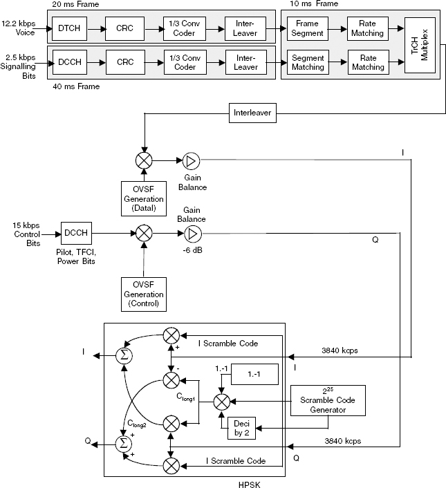
Figure 3.24 Uplink block diagram.

The complex scrambling applied to the uplink is a process known as Walsh rotation, which effectively continuously rotates the modulation constellation to reduce the PAR of the signal prior to modulation. It is also known as Hybrid Phase Shift Keying (HPSK) or sometimes orthogonal complex quadrature phase shift keying. HPSK allows handsets to transmit multiple channels at different amplitude levels while still maintaining acceptable peak-to-average power ratios.

Unlike the uplink, where the control bits are modulated onto the Q channel, the downlink multiplexes voice bits, signaling bits, and control bits together across the I and Q channels with slightly different rates resulting; voice and signaling bits are at 42 kbps, and pilot, power control, and TFCI control bits are at 18 kbps to give the 60 kbps channel rate.

Conformance/Performance Tests

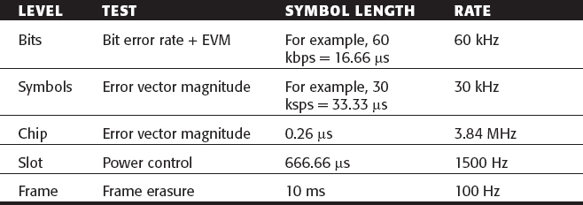
You can examine handset and Node B performance at bit level, symbol level, chip level, slot level, and frame level (as shown in Table 3.8), with the Node B exercised by any one of the four reference measurement channels (12.2, 64, 144, and 384 kbps) and the handset exercised by any one of five measurement channels (12.2, 64, 144, 384, and 786 kbps).

The measurement terms are E_b = energy in a user information bit, E_c = energy in every chip, E_b/N_o = ratio of bit energy to noise energy, and I_O = interference + noise density. You will also see the term E_b/N_t used to describe the narrowband thermal noise (for example, in adaptive RAKE design).

Chip level error vector magnitude includes spreading and HPSK scrambling. It cannot be used to identify OVSF or HPSK scrambling errors, but it can be used to detect baseband filtering, modulation, or RF impairments (the analog sections of the transmitter). It could, for example, be used to identify an I/Q quadrature error causing constellation distortion.

QPSK EVM measurement can be used to measure single DPDCH channels, but we are more interested in representing the effect of complex channels. This is done using the composite EVM measurement (3GPP modulation accuracy conformance test), as shown in Figure 3.25.

Table 3.8 Conformance Performance Tests

A reference signal is synthesized, downconverted (I and Q recovery), and passed through an RRC filter. Active channels are then descrambled, despread, and Binary Phase Shift Key (BPSK) decoded down to bit level. The despread bits are perfectly remodulated to obtain a reference signal to produce an error vector. Composite EVM can be used to identify all active channel spreading and scrambling problems and all baseband, IF, and RF impairments in the Tx chain.

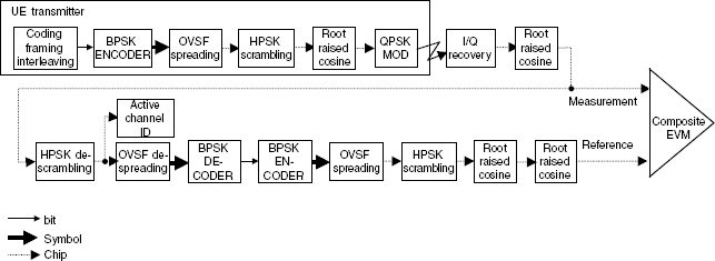
Figure 3.25 Composite EVM (bit-level EVM).

Impact of Technology Maturation on Handset and Network Performance

As devices improve and as design techniques improve handset sensitivity improves. There is also a performance benefit conferred by volume: better control of component tolerance. This could be observed as GSM matured over a 15-year period.

A similar performance evolution can be expected with IMT2000. Effectively the first two generations of cellular have followed a 15-year maturation cycle. It is reasonable to expect 3G technologies to follow a similar cycle.

3GPP2 Evolution

We have spent some time (some U.S. readers may say too much time) on the IMT2000DS/W-CDMA air interface. It is time to review the parallel evolution of CDMA2000/IS95. CDMA2000 is the term used to describe the air interface. IS2000 comprehends the air interface and network interfaces (interfaces to the IS41 network). Table 3.9 shows how IS95A/B has evolved with the adoption of variable length Walsh codes, use of QPSK on the downlink and HPSK on the uplink, more granular power control, supplemental code channels (multiple per-user channels on the downlink and uplink—one fundamental, up to seven supplemental), the option of multiple RF channels within a 5 MHz channel spacing (3xRTT), and the option of higher-level modulation (1xEV).

RC refers to radio configuration and specifies a set of data rates, spreading rates (SR) and coding.

In practice, it seems unlikely that 3xRTT will be implemented, and most deployment is presently focused on 1xEV using the present spreading rate of 1.288 Mcps as the most logical forward-evolution path. It may also be that fixed-length Walsh codes are used rather than variable length—variable data rates can be supported through adaptive modulation. However, variable-length Walsh codes do remain as an option in the standard.

Table 3.9 3GPP2 Evolution

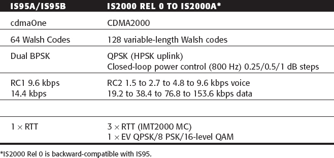
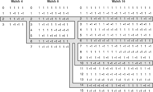
Figure 3.26 Variable length Walsh codes.

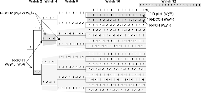
Figure 3.27 Reverse link code structure.

The length of the Walsh code is varied—from 4 to 128 chips—to accommodate different data rates. As the data rate increases, the symbol period gets shorter. The final chip rate stays constant—that is, fewer Walsh code chips are accommodated within the symbol period. If you re-order the code channels so that related code channels are adjacent to each other, you will have reproduced the OVSF code tree used in W-CDMA!

Figure 3.26 shows how, by rearranging the Walsh code tree you end up with an OVSF code tree. The dark portion represents a branch of the OVSF code tree.

As with W-CDMA, the use of HPSK on the uplink restricts which Walsh codes can be used to still keep PAR within acceptable limits. All the light gray codes shown in Figure 3.27. are nonorthogonal to the selected (dark gray) codes.

Table 3.10 gives examples of bit rate versus Walsh code length. Multiplying the code length by the data rate gives you the code rate.

Table 3.10 Bit Rate and Walsh Code Cover

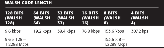
CDMA2000 Downlink and Uplink Comparison

The CDMA2000 downlink has not changed significantly from cdmaOne (IS95). There is one forward fundamental channel (F-FCH) and up to eight forward supplemental code channels (for RC2).

The uplink is significantly different because of the decision that handsets should be capable of transmitting more than one code simultaneously (a multicode uplink). This requires a reverse pilot (R-Pilot + power control), which allows the base station to do synchronous detection, and a reverse fundamental channel (R-FCH) for voice. Other supplemental channels (R-SCH) can be added in as required. The RDCCH (reverse dedicated control channel) is used to send data or signaling information. The channels can be assigned to either the I or the Q path and then complex-scrambled to generate the HPSK signal for modulation, to reduce the peak-to-average ratio.

Implementation Options

The original proposal from 3GPP2 to the ITU was based on the assumed need to fill 5 MHz of RF bandwidth. This could be achieved either by increasing the spreading ratio, as in SR3DS (direct sequence) shown in Figure 3.28, or by putting three CDMA2000 1.25 MHz channels together (SR3MC).

In practice, CDMA2000 is not being implemented into 5 MHz channels, and higher data rates are being achieved by using higher-level modulation schemes (8 PSK and 16-level QAM) in 1.25 MHz RF channels—the variant known as 1xEV.

Linearity and Modulation Quality

If higher levels of modulation are to be supported together with multiple codes per user on the uplink, then significant attention must be paid to PA linearity, both in the handset and the base station, if clipping is to be avoided. As mentioned, each coded channel represents a phase argument. The phase argument can be compromised by a loss of code-to-code orthogonality or AM to PM effects introduced by a PA in compression. It is important also to keep the code power well contained.

On the downlink, the BTS specification specifies that 91.2 percent of the correlated pilot power should be contained in the total transmission power. This means that 8.8 percent of the power produced potentially causes interference to other Walsh channels and embarrassment to the handset receive process.

As with IMT2000DS, modulation quality equates directly to capacity and coverage capability. Modulation quality in CDMA2000 is measured using RHO (equivalent to EVM). Causes of poor RHO could include RF PA compression, amplitude and phase errors in the IQ modulators, carrier feed-through, and spurious Tx signals.

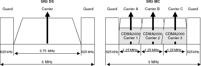
Figure 3.28 Implementation options for a 5 MHz channel.

Frequency Tolerance

Frequency tolerance also needs to be tightly specified. Failure of a GPS receiver will isolate a base station. The base station will still serve local handsets but will drift away from the rest of the network and become invisible—an island cell that takes with it the handsets it is presently supporting. Table 3.11 describes permitted frequency tolerance.

In IMT2000DS, a short code is used to bring the handset onto channel in terms of time synchronization. This helps to relax the frequency reference in the handset (reducing RF component count) but makes the long code acquisition process quite complex.

CDMA2000 is much simpler. All base stations share the same long code, but each base station is offset by 64 chips from the next base station. There are 512 possible offsets. When the handset is turned on, it should lock onto the long code with the shortest PN offset, because this will be, by implication, the nearest base station in terms of flight path.

The only disadvantage to this is that CDMA2000 timing errors need to be carefully managed to maintain acquisition performance and prevent false acquisition. A timing error in the offset higher than 3 μs can cause system performance degradation.

The orthogonality of Walsh codes and OVSF codes disappears if the codes are not time-aligned. Sources of timing errors can be within the application-specific integrated circuit (ASIC); time adjustment parameters), and delay in baseband signal paths or Walsh code intermodulation. The pilot to Walsh channel time tolerance is specified at <50 ns.

Table 3.11 Frequency Tolerance

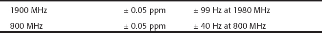
Phase errors between the receiver local oscillator and decorrelated Walsh channels create IQ interference and Walsh code intermodulation. The phase tolerance must be less than 2.86 degrees (50 milli-radians). The CDMA2000 handset uses the pilot channel phase as a reference. If the pilot channel phase is not aligned with the traffic channels, the traffic channels will not be demodulated!

Frequency/Power Profile

As with IMT2000DS, CDMA2000 is tightly specified in terms of spurious emissions, measured both for their impact in-band and out-of-channel, as shown in Figure 3.29.

In markets with legacy 30 kHz channel-spaced networks (US TDMA 800 MHz and 1900 MHz), adjacent channel power ratios need to be qualified with respect to adjacent narrowband channels. Similar specifications are required for out-of-band performance. The CDMA2000 specification requires spurious emissions outside the allocated system band (measured in a 30 kHz bandwidth) to be 60 dB below the mean output power in the channel bandwidth or −13 dBm, whichever is smaller.

Frame erasure rate can be used as a measure of receiver performance, provided coding and error correction is applied equally to all bits—that is, there are not classes of bits with different levels of error correction. Frame erasure rate is the ratio of the number of frames of data received that are deleted because of an unacceptable number of errors to the total number of frames transmitted. Frame erasure rate is used as a measure of receiver performance.

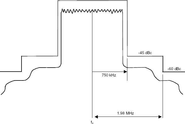
Figure 3.29 In-band/out-of-channel measurements.

We can use frame erasure rate to measure sensitivity and dynamic range, spurious immunity, and performance in AWGN and fading channels. CDMA2000 uses 20 ms frames. Base station receiver performance is expressed in terms of FER versus E_b /N_o. The E_b /N_o required will be a function of data rate and channel requirements.

At system level, the use of a continuous pilot in CDMA2000 provides better channel sounding, compared to IMT2000DS, but it uses more transmit energy. The continuous common pilot channel provides the following:

• More accurate estimation of the fading channel
• Faster detection of weak multipath rays than the per-user pilot approach
• Less overhead per user

Turbo coding is used for higher data rates with K = 9 constraint length.

The forward link coding is adaptive. Interleaving can either be 20 or 5 ms. A 6-bit, 8-bit, 10-bit, 12-bit, or 16-bit CRC is used for frame error checking with 1/2, 1/3, 1/4 rate K=9 convolutional coding. Equivalent rate turbo codes are used on supplemental channels. Each supplemental channel may use a different encoding scheme. Similarly, downlink coding is adaptive, using a 6-bit, 8-bit, 10-bit, 12-bit, or 16-bit CRC for frame error checking, and 9/16, 1/2, 1/3, 1/4 rate K=9 convolutional coding. Equivalent rate turbo codes are used on supplemental channels. Each supplemental channel may use a different encoding scheme. Interleaving is again either 5 ms or 20 ms.

Closed-loop power control is carried out at an 800 Hz control rate. The open loop sets Tx power level based on the Rx power received by the mobile and compensates for path loss and slow fading. The closed loop is for medium to fast fading and provides compensation for open-loop power control inaccuracies. The outer loop is implementation-specific and adjusts the closed-loop control threshold in the base station to maintain the desired frame error rate. The step size is adaptive, either 1 dB, 0.5 dB, or 0.25 dB. As with IMT2000DS, power control errors will directly subtract from the link budget.

The power control dynamic range is as follows:

• Open loop ±40 dB
• Closed loop ±24 dB

Power control errors are typically 1.3 dB (low mobility) or 2.7 dB (high mobility).

Dynamic range is similar to other existing networks:

Mobile	79 dB
Base station	52 dB
FDD isolation	(45 MHz, 800 MHz, 80 MHz at 1900 MHz)
Class II mobile	55 dB Tx to Rx
Base	90 dB (higher effective power, 5 dB lower noise floor)

Class IV handsets are equivalent to Power Class 3 handsets in IMT2000DS (250 mW). Class V handsets are equivalent to Power Class 4 handsets in IMT2000DS (125 mW). Both networks also support higher-power mobiles.

Class I:	28 dBm < EIRP < 33 dBm (2 W)
Class II:	23 dBm < EIRP < 30 dBm
Class III:	18 dBm < EIRP < 27 dBm
Class IV:	13 dBm < EIRP < 24 dBm (250 mW)
Class V:	8 dBm < EIRP <21 dBm (125 mW)

CDMA 1xEV has a high data rate option for the downlink, separate 1.25 MHz RF channel, QPSK, 8 PSK, 16-level QAM, and evolution to meet IMT2000MC requirements (3xRTT). 1xEV adds adaptive modulation as a mechanism for increasing data throughput.

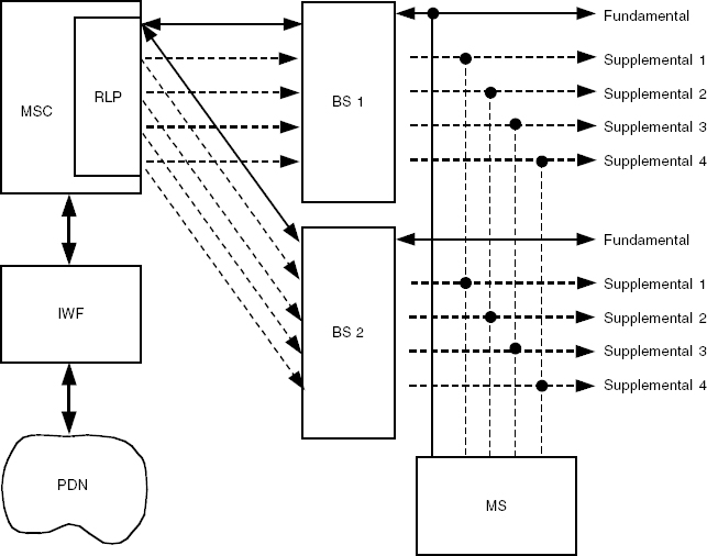
Figure 3.30 CDMA2000 handset in a soft handoff.

The Media Access Control (MAC) layer in IS2000 manages code allocation (the provision of physical layer resources to meet application layer requirements). An active high-rate mobile assigned a fundamental channel on origination negotiates high data rate service parameters. The mobile then sleeps but remains locked to a low-rate channel for synchronization and power control.

The handset signals a high data burst request by indicating to the base station (BS) its data backlog and maximum data rate requested. The handset includes pilot strength information for cells in its neighbor list, which indicates local interference levels. Additionally pilot strength measurements allow the base station to qualify instantaneous downlink capacity.

Supplemental code channels can then be allocated as required. In Figure 3.30, the handset communicates on the fundamental code channel with two base stations (BS1 and BS2). During a burst transmission, one or more supplemental code channels are assigned at BS1, BS2, or both. The MSC performs distribution on the forward link and selection on the reverse link. The Radio Link Protocol (RLP) does an Automatic Repeat Request (ARQ) and the interworking function (IWF) provides access to the packet data network.

When there is backlogged data, the mobile goes into active mode. If backlogged data exceeds a threshold, the mobile requests a supplementary channel (SCRM), sent on the fundamental code channel. The BS/MSC uses pilot strength measurements made by the mobile to decide on burst admission control and allocates supplementary channels. When backlogged data at the IWF exceeds a predetermined threshold, the IWF initiates a request for supplementary channels. The mobile is paged if not already in an active state.

In IS95B, a mobile is either active or dormant, and in CDMA2000, a handset can go into control hold, maintaining a dedicated control channel and power control (burst transmission with no added latency). In suspended state, there are no dedicated channels, although a virtual set of channels are maintained. In dormant state, there are no pre-allocated resources; in other words, the deeper the sleep, the lower the power consumption, but the longer it takes to wake up.

Summary

In this chapter we summarized the main tasks that need to be performed by a 3G handset, and we qualified code domain, frequency domain, and time domain performance issues. Typically, over a 15-year maturation cycle, handset performances improves on a year-by-year basis. and this delivers benefits in terms of network bandwidth quality.

In the following two chapters, we consider 3G handset hardware form factor and functionality and handset hardware evolution.