
CHAPTER 3 Discrete Revolution
Digital signal processing has taken over. First used in the 1950s at the service of analog signal processing to simulate analog transforms, digital algorithms have invaded most traditional fortresses, including phones, music recording, cameras, televisions, and all information processing. Analog computations performed with electronic circuits are faster than digital algorithms implemented with microprocessors but are less precise and less flexible. Thus, analog circuits are often replaced by digital chips once the computational performance of microprocessors is sufficient to operate in real time for a given application.
Whether sound recordings or images, most discrete signals are obtained by sampling an analog signal. An analog-to-digital conversion is a linear approximation that introduces an error dependent on the sampling rate. Once more, the Fourier transform is unavoidable because the eigenvectors of discrete time-invariant operators are sinusoidal waves. The Fourier transform is discretized for signals of finite size and implemented with a fast Fourier transform (FFT) algorithm.
3.1 SAMPLING ANALOG SIGNALS
The simplest way to discretize an analog signal f is to record its sample values ![]() at interval s. An approximation of f(t) at any t ∈
at interval s. An approximation of f(t) at any t ∈ ![]() may be recovered by interpolating these samples. The Shannon-Whittaker sampling theorem gives a sufficient condition on the support of the Fourier transform f to recover f(t) exactly. Aliasing and approximation errors are studied when this condition is not satisfied.
may be recovered by interpolating these samples. The Shannon-Whittaker sampling theorem gives a sufficient condition on the support of the Fourier transform f to recover f(t) exactly. Aliasing and approximation errors are studied when this condition is not satisfied.
Digital-acquisition devices often do not satisfy the restrictive hypothesis of the Shannon-Whittaker sampling theorem. General linear analog-to-discrete conversion is introduced in Section 3.1.3, showing that a stable uniform discretization is a linear approximation. A digital conversion also approximates discrete coefficients, with a given precision, to store them with a limited number of bits. This quantization aspect is studied in Chapter 10.
3.1.1 Shannon-Whittaker Sampling Theorem
Sampling is first studied from the more classic Shannon-Whittaker point of view, which tries to recover f(t) from its samples ![]() . A discrete signal can be represented as a sum of Diracs. We associate to any sample f(ns) a Dirac f(ns)δ(t – ns) located at t = ns. A uniform sampling of f thus corresponds to the weighted Dirac sum
. A discrete signal can be represented as a sum of Diracs. We associate to any sample f(ns) a Dirac f(ns)δ(t – ns) located at t = ns. A uniform sampling of f thus corresponds to the weighted Dirac sum
 (3.1)
(3.1)The Fourier transform of δ(t – ns) is e−insω, so the Fourier transform of fd is a Fourier series:
 (3.2)
(3.2)To understand how to compute f(t) from the sample values f(ns) and therefore f from fd, we relate their Fourier transforms ![]() and
and ![]() .
.
Theorem 3.1.
The Fourier transform of the discrete signal obtained by sampling f at interval s is
 (3.3)
(3.3)Proof.
Since S(t – ns) is zero outside t = ns,
we can rewrite (3.1) as multiplication with a Dirac comb:
Computing the Fourier transform yields
The Poisson formula (2.4) proves that
 (3.6)
(3.6)Since ![]() , inserting (3.6) into (3.5) proves (3.3).
, inserting (3.6) into (3.5) proves (3.3).
Theorem 3.1 proves that sampling f at interval s is equivalent to making its Fourier transform 2π/s periodic by summing all its translations ![]() . The resulting sampling theorem was first proved by Whittaker [482] in 1935 in a book on interpolation theory. Shannon rediscovered it in 1949 for applications to communication theory [429].
. The resulting sampling theorem was first proved by Whittaker [482] in 1935 in a book on interpolation theory. Shannon rediscovered it in 1949 for applications to communication theory [429].
Theorem 3.2:
Shannon, Whittaker. If the support of f is included in [–π/s, π/s], then
Proof.
If n ≠ 0, the support of ![]() does not intersect the support of
does not intersect the support of ![]() because
because ![]() ; so (3.3) implies
; so (3.3) implies
The Fourier transform of ϕs is ![]() . Since the support of
. Since the support of ![]() is in [–π/s, π/s], it results from (39) that
is in [–π/s, π/s], it results from (39) that ![]() . The inverse Fourier transform of this equality gives
. The inverse Fourier transform of this equality gives

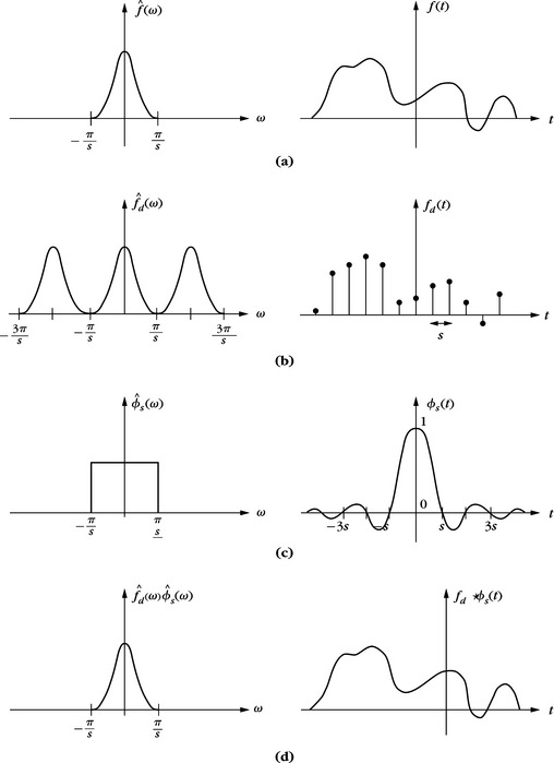
The sampling theorem supposes that the support of ![]() is included in [–π/s, π/s], which guarantees that f has no brutal variations between consecutive samples; thus, it can be recovered with a smooth interpolation. Section 3.1.3 shows that one can impose other smoothness conditions to recover f from its samples. Figure 3.1 illustrates the different steps for a sampling and reconstruction from samples, in both the time and Fourier domains.
is included in [–π/s, π/s], which guarantees that f has no brutal variations between consecutive samples; thus, it can be recovered with a smooth interpolation. Section 3.1.3 shows that one can impose other smoothness conditions to recover f from its samples. Figure 3.1 illustrates the different steps for a sampling and reconstruction from samples, in both the time and Fourier domains.
3.1.2 Aliasing
The sampling interval s is often imposed by computation or storage constraints and support of ![]() is generally not included in [–π/s, π/s]. In this case the interpolation formula (37) does not recover f. We analyze the resulting error and a filtering procedure to reduce it.
is generally not included in [–π/s, π/s]. In this case the interpolation formula (37) does not recover f. We analyze the resulting error and a filtering procedure to reduce it.
Theorem 3.1 proves that
 (3.10)
Suppose that support of ![]() goes beyond [–π/s, π/s]. In general, support of
goes beyond [–π/s, π/s]. In general, support of ![]() intersects [–π/s, π/s] for several k ≠ 0, as shown in Figure 3.2. This folding of high-frequency components over a low-frequency interval is called aliasing. In the presence of aliasing, the interpolated signal
intersects [–π/s, π/s] for several k ≠ 0, as shown in Figure 3.2. This folding of high-frequency components over a low-frequency interval is called aliasing. In the presence of aliasing, the interpolated signal

FIGURE 3.2 (a) Signal f and its Fourier transform ![]() (b) Aliasing produced by an overlapping of
(b) Aliasing produced by an overlapping of ![]() (ω – 2kπ/s) for different k, shown with dashed lines. (c) Ideal low-pass filter. (d) The filtering of (b) with (c) creates a low-frequency signal that is different from f.
(ω – 2kπ/s) for different k, shown with dashed lines. (c) Ideal low-pass filter. (d) The filtering of (b) with (c) creates a low-frequency signal that is different from f.

 (3.11)
which may be completely different from ![]() over [–π/s, π/s]. The signal
over [–π/s, π/s]. The signal ![]() may not even be a good approximation of f, as shown by Figure 3.2.
may not even be a good approximation of f, as shown by Figure 3.2.
EXAMPLE 3.1
Let us consider a high-frequency oscillation
If 2π/s > ω0 > π/s, then (3.11) yields
The aliasing reduces the high-frequency ω0 to a lower frequency 2π/s – ω0 ∈ [–π/s, π/s]. The same frequency folding is observed in a film that samples a fast-moving object without enough images per second. A wheel turning rapidly appears as though turning much more slowly in the film.
Removal of Aliasing
To apply the sampling theorem, f is approximated by the closest signal ![]() , the Fourier transform of which has a support in [–π/s, π/s]. The Plancherel formula (2.26) proves that
, the Fourier transform of which has a support in [–π/s, π/s]. The Plancherel formula (2.26) proves that

This distance is minimum when the second integral is zero and therefore
The filtering of f by ϕs avoids aliasing by removing any frequency larger than π/s. Since ![]() has a support in [–π/s, π/s], the sampling theorem proves that ˜(t) can be recovered from the samples ˜(ns). An analog-to-digital converter is therefore composed of a filter that limits the frequency band to [–π/s, π/s], followed by a uniform sampling at interval s.
has a support in [–π/s, π/s], the sampling theorem proves that ˜(t) can be recovered from the samples ˜(ns). An analog-to-digital converter is therefore composed of a filter that limits the frequency band to [–π/s, π/s], followed by a uniform sampling at interval s.
3.1.3 General Sampling and Linear Analog Conversions
The Shannon-Whittaker theorem is a particular example of linear discrete-to-analog conversion, which does not apply to all digital acquisition devices. This section describes general analog-to-discrete conversion and reverse discrete-to-analog conversion, with general linear filtering and uniform sampling. Analog signals are approximated by linear projections on approximation spaces.
Sampling Theorems
We want to recover a stable approximation of f ∈ L2 (![]() ) from a filtering and uniform sampling, which outputs
) from a filtering and uniform sampling, which outputs ![]() , for some real filter
, for some real filter ![]() . These samples can be written as inner products in L2 (
. These samples can be written as inner products in L2 (![]() ):
):
with ![]() . Let Us be the approximation space generated by linear combination of the
. Let Us be the approximation space generated by linear combination of the ![]() . The approximation f ∈ Us, which minimizes the maximum possible error ‖f – f‖, is the orthognal projection of f on Us (Exercice 3.5). The calculation of this orthogonal projection is stable if
. The approximation f ∈ Us, which minimizes the maximum possible error ‖f – f‖, is the orthognal projection of f on Us (Exercice 3.5). The calculation of this orthogonal projection is stable if ![]() is a Riesz basis of Us, as defined in Section 5.1.1.
is a Riesz basis of Us, as defined in Section 5.1.1.
Following Definition 5.1, a Riesz basis is a family of linearly independent functions that yields an inner product satisfying an energy equivalence. There exists B ≥ A > 0 such that for any f ∈ Us
 (3.14)
The basis is orthogonal if and only if A = B. The following generalized sampling theorem computes the orthogonal projection on the approximation space Us [468].
Theorem 3.3:
Linear sampling. Let ![]() be a Riesz basis of Us and
be a Riesz basis of Us and ![]() . There exists a biorthogonal basis
. There exists a biorthogonal basis ![]() of Us such that
of Us such that
 (3.15)
Proof.
For any Riesz basis, Section 5.1.2 proves that a biorthogonal basis ![]() exists that satisfies the biorthogonality relations
exists that satisfies the biorthogonality relations
Since ![]() and since the dual basis is unique, necessarily
and since the dual basis is unique, necessarily ![]() . Section 5.1.2 proves in (5.20) that the orthogonal projection in Us can be written
. Section 5.1.2 proves in (5.20) that the orthogonal projection in Us can be written

which proves (3.15).
The orthogonal projection (3.15) can be rewritten as an analog filtering of the discrete signal ![]() :
:
If f ∈ Us, then ![]() so it is exactly reconstructed by filtering the uniformly sampled discrete signal
so it is exactly reconstructed by filtering the uniformly sampled discrete signal ![]() with the analog filter
with the analog filter ![]() . If f ∈ Us, then (3.17) recovers the best linear approximation of f in Us. Section 9.1 shows that the linear approximation error
. If f ∈ Us, then (3.17) recovers the best linear approximation of f in Us. Section 9.1 shows that the linear approximation error ![]() essentially depends on the uniform regularity of f. Given some prior information on f, optimizing the analog discretization filter ϕs amounts to optimizing the approximation space Us to minimize this error. The following theorem characterizes filters ϕs that generate a Riesz basis and computes the dual filter.
essentially depends on the uniform regularity of f. Given some prior information on f, optimizing the analog discretization filter ϕs amounts to optimizing the approximation space Us to minimize this error. The following theorem characterizes filters ϕs that generate a Riesz basis and computes the dual filter.
Theorem 3.4.
A filter ϕs generates a Riesz basis ![]() of a space Us if and only if there exists B ≥ A > 0 such that
of a space Us if and only if there exists B ≥ A > 0 such that
 (3.18)
The biorthogonal basis ![]() is defined by the dual filter
is defined by the dual filter ![]() , which satisfies:
, which satisfies:
Proof.
Theorem 5.5 proves that ![]() is a Riesz basis of Us with Riesz bounds B ≥ A > 0 if and only if it is linearly independent and
is a Riesz basis of Us with Riesz bounds B ≥ A > 0 if and only if it is linearly independent and
Let us first write these conditions in the Fourier domain. The Fourier transform of ![]() is
is
 (3.21)
where â(ω) is the Fourier series ![]() . Let us relate the norm of f and â. Since â(ω) is 2π/s periodic, inserting (3.21) in the Plancherel formula (2.26) gives
. Let us relate the norm of f and â. Since â(ω) is 2π/s periodic, inserting (3.21) in the Plancherel formula (2.26) gives
 (3.22)
Section 3.2.2 on Fourier series proves that
 (3.23)
As a consequence of (3.22) and (3.23), the Riesz bound inequalities (3.20) are equivalent to
If ![]() satisfies (3.18), then clearly (3.24) and (3.25) are valid, which proves (3.22).
satisfies (3.18), then clearly (3.24) and (3.25) are valid, which proves (3.22).
Conversely, if ![]() is a Riesz basis. Suppose that either the upper or the lower bound of (3.18) is not satisfied for ω in a set of nonzero measures. Let â be the indicator function of this set. Then either (3.24) or (3.25) is not valid for this â. This implies that the Riesz bounds (3.20) are not valid for a and therefore that it is not a Riesz basis, which contradicts our hypothesis. So (3.18) is indeed valid for almost all ω ∈ [0, 2π/s].
is a Riesz basis. Suppose that either the upper or the lower bound of (3.18) is not satisfied for ω in a set of nonzero measures. Let â be the indicator function of this set. Then either (3.24) or (3.25) is not valid for this â. This implies that the Riesz bounds (3.20) are not valid for a and therefore that it is not a Riesz basis, which contradicts our hypothesis. So (3.18) is indeed valid for almost all ω ∈ [0, 2π/s].
To compute the biorthogonal basis, we are looking for ![]() such that
such that ![]() satisfies the biorthogonal relations (3.16). Since
satisfies the biorthogonal relations (3.16). Since ![]() we saw in (3.21) that its Fourier transform can be written
we saw in (3.21) that its Fourier transform can be written ![]() , where â(ω) is 2π/s periodic. Let us define
, where â(ω) is 2π/s periodic. Let us define ![]() . Its Fourier transform is
. Its Fourier transform is
The biorthogonal relations (3.16) are satisfied if and only if g(ns) = 0 if n ≠ 0 and g(0) = 1. It results that ![]() . Theorem 3.1 derives in (3.3) that
. Theorem 3.1 derives in (3.3) that

which proves (3.19).
This theorem gives a necessary and sufficient condition on the low-pass filter ![]() to recover a stable signal approximation from uniform sampling at interval s. For various sampling interval s, the low-pass filter can be obtained by dilating a single filter
to recover a stable signal approximation from uniform sampling at interval s. For various sampling interval s, the low-pass filter can be obtained by dilating a single filter ![]() and thus
and thus ![]() . The necessary and sufficient Riesz basis condition (3.18) is then satisfied if and only if
. The necessary and sufficient Riesz basis condition (3.18) is then satisfied if and only if
 (3.26)
It results from (3.19) that the dual filter satisfies ![]() and therefore
and therefore ![]() . When A = B = 1, the Riesz basis is an orthonormal basis, which proves Corollary 3.1.
. When A = B = 1, the Riesz basis is an orthonormal basis, which proves Corollary 3.1.
 (3.27)
Shannon-Whittaker Revisited
Shannon-Whittaker, Theorem 3.2, is defined with a sine-cardinal perfect low-pass filter ϕs, which we renormalize here to have a unit norm. The following theorem proves that it samples functions on an orthonormal basis.
Theorem 3.5.
If ϕs(t) = s1/2 sin(πs−1 t)/(πt) then ![]() is an orthonormal basis of the space Us of functions whose Fourier transforms have a support included in [–π/s, π/s]. If f ∈ Us, then
is an orthonormal basis of the space Us of functions whose Fourier transforms have a support included in [–π/s, π/s]. If f ∈ Us, then
Proof.
The filter satisfies ϕs(t) = s−1/2 ϕ(t/s) with ϕ(t) = sin(πt)/(πt). The Fourier transform ![]() satisfies the condition (3.27) of Corollary 3.1, which proves that
satisfies the condition (3.27) of Corollary 3.1, which proves that ![]() is an orthonormal basis of a space Us.
is an orthonormal basis of a space Us.
Any ![]() has a Fourier transform that can be written
has a Fourier transform that can be written
 (3.29)
which implies that f ∈ Us if and only if f has a Fourier transform supported in [–π/s, π/s].
If f ∈ Us, then decomposing it on the orthonormal basis ![]() gives
gives
Since ϕs(ps) = s−1/2δ[ps] and ϕs(–t) = ϕs(t), the result is that
This theorem proves that in the particular case of the Shannon-Whittaker sampling theorem, if f ∈ Us then the sampled low-pass filtered values ![]() are proportional to the signal samples f(ns). This comes from the fact that the sine-cardinal ϕ(t) = sin(πt/s)/(πt/s) satisfies the interpolation property ϕ(ns) = δ[ns]. A generalization of such multiscale interpolations is studied in Section 7.6.
are proportional to the signal samples f(ns). This comes from the fact that the sine-cardinal ϕ(t) = sin(πt/s)/(πt/s) satisfies the interpolation property ϕ(ns) = δ[ns]. A generalization of such multiscale interpolations is studied in Section 7.6.
Shannon-Whittaker sampling approximates signals by restricting their Fourier transform to a low-frequency interval. It is particularly effective for smooth signals with a Fourier transform that has energy concentrated at low frequencies. It is also adapted for sound recordings, which are sufficiently approximated by lower-frequency harmonics.
For discontinuous signals, such as images, a low-frequency restriction produces Gibbs oscillations, as described in Section 2.3.3. The image visual quality is degraded by these oscillations, which have a total variation (2.65) that is infinite. A piecewise constant approximation has the advantage of creating no such spurious oscillations.
Block Sampler
A block sampler approximates signals with piecewise constant functions. The approximation space Us is the set of all functions that are constant on intervals [ns, (n + 1)s], for any n ∈ ![]() . Let ϕs(t) = s−1/2 1[0,s](t). The family
. Let ϕs(t) = s−1/2 1[0,s](t). The family ![]() is an orthonormal basis of Us (Exercise 3.1). If f ∈ Us, then its orthogonal projection on Us is calculated with a partial decomposition in the block orthonormal basis of Us
is an orthonormal basis of Us (Exercise 3.1). If f ∈ Us, then its orthogonal projection on Us is calculated with a partial decomposition in the block orthonormal basis of Us
and each coefficient is proportional to the signal average on [ns, (n + 1)s]:
This block analog-to-digital conversion is particularly simple to implement in analog electronics, where integration is performed by a capacity.
In domains where f is a regular function, a piecewise constant approximation ![]() is not very precise and can be significantly improved. More precise approximations are obtained with approximation spaces Us of higher-order polynomial splines. The resulting approximations can introduce small Gibbs oscillations, but these oscillations have a finite total variation.
is not very precise and can be significantly improved. More precise approximations are obtained with approximation spaces Us of higher-order polynomial splines. The resulting approximations can introduce small Gibbs oscillations, but these oscillations have a finite total variation.
Spline Sampling
Block samplers are generalized by spline sampling with a space Us of spline functions that are m – 1 times continuously differentiable and equal to a polynomial of degree m on any interval [ns, (n + 1)s), for n ∈ ![]() . When m = 1, functions in Us are piecewise linear and continuous.
. When m = 1, functions in Us are piecewise linear and continuous.
A Riesz basis of polynomial splines is constructed with box splines. A box spline ϕ of degree m is computed by convolving the box window 1[0,1] with itself m + 1 times and centering it at 0 or 1/2. Its Fourier transform is
If m is even, then ε = 1 and ϕ have a support centered at t = 1/2. If m is odd, then ε = 0 and ϕ(t) are symmetric about t = 0. One can verify that ![]() satisfies the sampling condition (3.26) using a closed-form expression (7.20) of the resulting series. This means that for any s > 0, a box splines family
satisfies the sampling condition (3.26) using a closed-form expression (7.20) of the resulting series. This means that for any s > 0, a box splines family ![]() defines a Riesz basis of Us, and thus is a stable sampling.
defines a Riesz basis of Us, and thus is a stable sampling.
3.2 DISCRETE TIME-INVARIANT FILTERS
3.2.1 Impulse Response and Transfer Function
Classic discrete signal-processing algorithms most generally are based on time-invariant linear operators [51, 55]. The time invariance is limited to translations on the sampling grid. To simplify notation, the sampling interval is normalized s = 1, and we denote f[n] the sample values. A linear discrete operator L is time-invariant if an input f[n], delayed by p ∈ ![]() , fp[n] = f[n – p], produces an output also delayed by p:
, fp[n] = f[n – p], produces an output also delayed by p:
Impulse Response
We denote by δ[n] the discrete Dirac
Any signal f[n] can be decomposed as a sum of shifted Diracs:
Let Lδ[n] = h[n] be the discrete impulse response. Linearity and time invariance implies that
 (3.33)
A discrete linear time-invariant operator is thus computed with a discrete convolution. If h[n] has a finite support, the sum (3.33) is calculated with a finite number of operations. These are called finite impulse response (FIR) filters. Convolutions with infinite impulse response filters may also be calculated with a finite number of operations if they can be rewritten with a recursive equation (3.45).
Causality and Stability
A discrete filter L is causal if Lf[p] depends only on the values of f[n] for n ≤ p. The convolution formula (333) implies that h[n] = 0 if n < 0.
The filter is stable if any bounded input signal f[n] produces a bounded output signal Lf[n]. Since

it is sufficient that ![]() , which means that h ∈
, which means that h ∈ ![]() 1(
1(![]() ). One can verify that this sufficient condition is also necessary. Thus, the filter is stable if and only if h ∈
). One can verify that this sufficient condition is also necessary. Thus, the filter is stable if and only if h ∈ ![]() 1(
1(![]() ) (Exercise 3.6).
) (Exercise 3.6).
 (3.34)
 (3.35)
 (3.36)
3.2.2 Fourier Series
The properties of Fourier series are essentially the same as the properties of the Fourier transform since Fourier series are particular instances of Fourier transforms for Dirac sums. If ![]() , then
, then ![]() .
.
For any n ∈ ![]() , e−iωn has period 2π, so Fourier series have period 2π. An important issue to understand is whether all functions with period 2π can be written as Fourier series. Such functions are characterized by their restriction to [–π, π]. We therefore consider functions â ∈ L2 [– π, π] that are square integrable over [–π, π]. The space L2 [– π, π] is a Hilbert space with the inner product
, e−iωn has period 2π, so Fourier series have period 2π. An important issue to understand is whether all functions with period 2π can be written as Fourier series. Such functions are characterized by their restriction to [–π, π]. We therefore consider functions â ∈ L2 [– π, π] that are square integrable over [–π, π]. The space L2 [– π, π] is a Hilbert space with the inner product
Theorem 3.6 proves that any function in L2[– π, π] can be written as a Fourier series.
Theorem 3.6.
The family of functions ![]() is an orthonormal basis of L2[–π, π].
is an orthonormal basis of L2[–π, π].
Proof.
The orthogonality with respect to the inner product (3.37) is established with a direct integration. To prove that ![]() is a basis, we must show that linear expansions of these vectors are dense in L2 [– π, π].
is a basis, we must show that linear expansions of these vectors are dense in L2 [– π, π].
We first prove that any continuously differentiable function ![]() with a support included in [–π, π] satisfies
with a support included in [–π, π] satisfies
 (3.38)
with a pointwise convergence for any ω ∈[–π, π]. Let us compute the partial sum

The Poisson formula (2.37) proves the distribution equality
and since the support of ![]() is in [–π, π], we get
is in [–π, π], we get
Since ![]() is continuously differentiable, following the steps (2.38–2.40) in the proof of the Poisson formula shows that SN(ω) converges uniformly to
is continuously differentiable, following the steps (2.38–2.40) in the proof of the Poisson formula shows that SN(ω) converges uniformly to ![]() (ω) on [–π, π].
(ω) on [–π, π].
To prove that linear expansions of sinusoidal waves ![]() are dense in L2[–π, π], let us verify that the distance between â ∈ L2[–π, π] and such a linear expansion is less than ε, for any ε > 0. Continuously differentiable functions with a support included in [–π, π] are dense in L2[–π, π]; thus, there exists
are dense in L2[–π, π], let us verify that the distance between â ∈ L2[–π, π] and such a linear expansion is less than ε, for any ε > 0. Continuously differentiable functions with a support included in [–π, π] are dense in L2[–π, π]; thus, there exists ![]() such that
such that ![]() . The uniform pointwise convergence proves that there exists N for which
. The uniform pointwise convergence proves that there exists N for which
It follows that â is approximated by the Fourier series SN with an error
Theorem 3.6 proves that if f ∈ ![]() 2(
2(![]() ), the Fourier series
), the Fourier series
 (3.39)
can be interpreted as the decomposition of ![]() in an orthonormal basis of L2 [– π, π]. The Fourier series coefficients can thus be written as inner products in L2 [– π, π]:
in an orthonormal basis of L2 [– π, π]. The Fourier series coefficients can thus be written as inner products in L2 [– π, π]:
The energy conservation of orthonormal bases (A.10) yields a Plancherel identity:
 (3.41)
Pointwise Convergence
The equality (3.39) is meant in the sense of mean-square convergence

It does not imply a pointwise convergence ![]()
In 1873, Dubois-Reymond constructed a periodic function ![]() that is continuous and has a Fourier series that diverges at some point. On the other hand, if
that is continuous and has a Fourier series that diverges at some point. On the other hand, if ![]() is continuously differentiable, then the proof of Theorem 3.6 shows that its Fourier series converges uniformly to
is continuously differentiable, then the proof of Theorem 3.6 shows that its Fourier series converges uniformly to ![]() on [–π, π]. It was only in 1966 that Carleson [149] was able to prove that if
on [–π, π]. It was only in 1966 that Carleson [149] was able to prove that if ![]() ∈ L2 [– π, π] then its Fourier series converges almost everywhere. The proof is very technical.
∈ L2 [– π, π] then its Fourier series converges almost everywhere. The proof is very technical.
Convolutions
Since ![]() are eigenvectors of discrete convolution operators, we also have a discrete convolution theorem.
are eigenvectors of discrete convolution operators, we also have a discrete convolution theorem.
Theorem 3.7.
If f ∈ ![]() 1 (
1 (![]() ) and h ∈
) and h ∈ ![]() 1 (
1 (![]() ), then
), then ![]() and
and
The proof is identical to the proof of the convolution, Theorem 2.2, if we replace integrals by discrete sums. The reconstruction formula (3.40) shows that a filtered signal can be written
The transfer function ĥ(ω) amplifies or attenuates the frequency components ![]() of f[n].
of f[n].
EXAMPLE 3.4
A recursive filter computes g = Lf, which is a solution of a recursive equation
 (3.45)
with b0 ≠ 0. If g[n] = 0 and f[n] = 0 for n < 0, then g has a linear and time-invariant dependency on f and thus can be written ![]() . The transfer function is obtained by computing the Fourier transform of (3.45). The Fourier transform of fk[n] = f[n – k] is
. The transfer function is obtained by computing the Fourier transform of (3.45). The Fourier transform of fk[n] = f[n – k] is ![]() so
so
It is a rational function of e−iω. If bk ≠ 0 for some k > 0, then one can verify that the impulse response h has an infinite support. The stability of such filters is studied in Exercise 3.18. A direct calculation of the convolution sum g[n] = f ![]() h[n] would require an infinite number of operations, whereas (3.45) computes g[n] with K + M additions and multiplications from its past values.
h[n] would require an infinite number of operations, whereas (3.45) computes g[n] with K + M additions and multiplications from its past values.
Window Multiplication
An infinite impulse response filter h, such as the ideal low-pass filter (3.44), may be approximated by a finite response filter h by multiplying h with a window g of finite support:
One can verify (Exercise 3.6) that a multiplication in time is equivalent to a convolution in the frequency domain:
Clearly ![]() only if ĝ = 2πδ, which would imply that g has an infinite support and g[n] = 1. The approximation
only if ĝ = 2πδ, which would imply that g has an infinite support and g[n] = 1. The approximation ![]() is close to ĥ only if ĝ approximates a Dirac, which means that all its energy is concentrated at low frequencies. In time, g should therefore have smooth variations.
is close to ĥ only if ĝ approximates a Dirac, which means that all its energy is concentrated at low frequencies. In time, g should therefore have smooth variations.
The rectangular window g = 1[–N, N] has a Fourier transform ĝ computed in (3.36). It has important side lobes far away from ω = 0. The resulting ![]() is a poor approximation of ĥ. The Hanning window
is a poor approximation of ĥ. The Hanning window
is smoother and thus has a Fourier transform better concentrated at low frequencies. The spectral properties of other windows are studied in Section 4.2.2.
3.3 FINITE SIGNALS
Up to now we have considered discrete signals f[n] defined for all n ∈ ![]() . In practice, f[n] is known over a finite domain, say 0 ≤ n < N. Convolutions therefore must be modified to take into account the border effects at n = 0 and n = N – 1. The Fourier transform also must be redefined over finite sequences for numerical computations. The fast Fourier transform algorithm is explained as well as its application to fast convolutions.
. In practice, f[n] is known over a finite domain, say 0 ≤ n < N. Convolutions therefore must be modified to take into account the border effects at n = 0 and n = N – 1. The Fourier transform also must be redefined over finite sequences for numerical computations. The fast Fourier transform algorithm is explained as well as its application to fast convolutions.
3.3.1 Circular Convolutions
Let f and h be signals of N samples. To compute the convolution product

we must know f[n] and h;[n] beyond 0 ≤ n < N. One approach is to extend f and h with a periodization over N samples, and to define
The circular convolution of two such signals, both with period N, is defined as a sum over their period:

It is also a signal of period N.
The eigenvectors of a circular convolution operator
are the discrete complex exponentials ek[n] = exp (i2πkn/N). Indeed,

and the eigenvalue is the discrete Fourier transform of h:
3.3.2 Discrete Fourier Transform
The space of signals of period N is an Euclidean space of dimension N and the inner product of two such signals f and g is
 (3.47)
Theorem 3.8 proves that any signal with period N can be decomposed as a sum of discrete sinusoidal waves.
Theorem 3.8.
is an orthogonal basis of the space of signals of period N.
Since the space is of dimension N, any orthogonal family of N vectors is an orthogonal basis. To prove this theorem, it is sufficient to verify that {ek}0≤k<N is orthogonal with respect to the inner product (3.47) (Exercise 3.8). Any signal f of period N can be decomposed on this basis:
 (3.48)
By definition, the discrete Fourier transform (DFT) of f is
 (3.49)
Since ‖ek‖2 = N, (3.48) gives an inverse discrete Fourier formula:
 (3.50)
The orthogonality of the basis also implies a Plancherel formula:
 (3.51)
The discrete Fourier tranform (DFT) of a signal f of period N is computed from its values for 0 ≤ n < N. Then why is it important to consider it a periodic signal with period N rather than a finite signal of N samples? The answer lies in the interpretation of the Fourier coefficients. The discrete Fourier sum (3.50) defines a signal of period N for which the samples f[0] and f[N – 1] are side by side. If f[0] and f[N – 1] are very different, this produces a brutal transition in the periodic signal, creating relatively high-amplitude Fourier coefficients at high frequencies. For example, Figure 3.3 shows that the “smooth” ramp f[n] = n for 0 ≤ n < N has sharp transitions at n = 0 and n = N once made periodic.

Circular Convolutions
Since {exp (i2πkn/N)}0≤k<N are eigenvectors of circular convolutions, we derive a convolution theorem.
Theorem 3.9.
If f and h have period N, then the discrete Fourier transform of ![]() is
is
The proof is similar to the proof of the two previous convolution theorems—2.2 and 3.7. This theorem shows that a circular convolution can be interpreted as a discrete frequency filtering. It also opens the door to fast computations of convolutions using the fast Fourier transform.
3.3.3 Fast Fourier Transform
For a signal f of N points, a direct calculation of the N discrete Fourier sums
 (3.53)
requires N2 complex multiplications and additions. The FFT algorithm reduces the numerical complexity to O(N log2N) by reorganizing the calculations.
When the frequency index is even, we group the terms n and n + N/2:
 (3.54)
When the frequency index is odd, the same grouping becomes
 (3.55)
Equation (3.54) proves that even frequencies are obtained by calculating the DFT of the N/2 periodic signal
Odd frequencies are derived from (355) by computing the Fourier transform of the N/2 periodic signal:
A DFT of size N may thus be calculated with two discrete Fourier transforms of size N/2 plus O(N) operations.
The inverse FFT of ![]() is derived from the forward fast Fourier transform of its complex conjugate
is derived from the forward fast Fourier transform of its complex conjugate ![]() by observing that
by observing that
 (3.56)
Complexity
Let C(N) be the number of elementary operations needed to compute a DFT with the FFT. Since f is complex, the calculation of fe and fo requires N complex additions and N/2 complex multiplications. Let KN be the corresponding number of elementary operations. We have
since the Fourier transform of a single point is equal to itself, C(1) = 0. With the change of variable l = log2 N and the change of function ![]() , from (3.57) we derive
, from (3.57) we derive
Since T(0) = 0, we get T(l) = K l and therefore
Several variations of this fast algorithm exist [49, 237]. The goal is to minimize the constant K. The most efficient fast DFT to this date is the split-radix FFT algorithm, which is slightly more complicated than the procedure just described; however; it requires only N log2 N real multiplications and 3N log2 N additions. When the input signal f is real, there are half as many parameters to compute, since ![]() [–k] =
[–k] = ![]() *[k]. The number of multiplications and additions is thus reduced by 2.
*[k]. The number of multiplications and additions is thus reduced by 2.
3.3.4 Fast Convolutions
The low computational complexity of a FFT makes it efficient to compute finite discrete convolutions by using the circular convolution, Theorem 3.9. Let f and h be two signals with samples that are nonzero only for 0 ≤ n < M. The causal signal
 (3.58)
is nonzero only for 0 ≤ n < 2M. If h and f have M nonzero samples, calculating this convolution product with the sum (3.58) requires M(M + 1) multiplications and additions. When M ≥ 32, the number of computations is reduced by using the FFT [11, 49].
To use the fast Fourier transform with the circular convolution, Theorem 3.9, the noncircular convolution (3.58) is written as a circular convolution. We define two signals of period 2M:
By letting ![]() , one can verify that c[n] = g[n] for 0 ≤ n < 2M. The 2M nonzero coefficients of g are thus obtained by computing â and
, one can verify that c[n] = g[n] for 0 ≤ n < 2M. The 2M nonzero coefficients of g are thus obtained by computing â and ![]() from a and b and then calculating the inverse DFT of ĉ = a b.
from a and b and then calculating the inverse DFT of ĉ = a b.
With the fast Fourier transform algorithm, this requires a total of O(M log2M) additions and multiplications instead of M(M + 1). A single FFT or inverse FFT of a real signal of size N is calculated with 2−1N log2 N multiplications, using a split-radix algorithm. The FFT convolution is thus performed with a total of 3M log2 M + 11M real multiplications. For M ≥ 32, the FFT algorithm is faster than the direct convolution approach. For M ≤ 16, it is faster to use a direct convolution sum.
Fast Overlap-Add Convolutions
The convolution of a signal f of L nonzero samples with a smaller causal signal h of M samples is calculated with an overlap-add procedure that is faster than the previous algorithm. The signal f is decomposed with a sum of L/M blocks fr having M nonzero samples:
 (3.61)
For each 0 ≤ r < L/M, the 2M nonzero samples of  are computed with the FFT-based convolution algorithm, which requires O(M log2 M) operations. These L/M convolutions are thus obtained with O(L log2 M) operations. The block decomposition (3.61) implies that
The addition of these L/M translated signals of size 2M is done with 2L additions. The overall convolution is thus performed with O(L log2 M) operations.
3.4 DISCRETE IMAGE PROCESSING
Two-dimensional signal processing poses many specific geometric and topological problems that do not exist in one dimension [21, 33]. For example, a simple concept, such as causality, is not well defined in two dimensions. We can avoid the complexity introduced by the second dimension by extending one-dimensional algorithms with a separable approach. This not only simplifies the mathematics but also leads to fast numerical algorithms along the rows and columns of images. Section A.5 in the Appendix reviews the properties of tensor products for separable calculations.
3.4.1 Two-Dimensional Sampling Theorems
The light intensity measured by a camera is generally sampled over a rectangular array of picture elements, called pixels. One-dimensional sampling theorems are extended to this two-dimensional sampling array. Other two-dimensional sampling grids such as hexagonal, are also possible, but nonrectangular sampling arrays are not used often.
Let s1 and s2 be the sampling intervals along the x1 and x2 axes of an infinite rectangular sampling grid. The following renormalizes the axes so that s1 = s2 = s. A discrete image obtained by sampling f(x) with x = (x1, x2) can be represented as a sum of Diracs located at the grid points:
The two-dimensional Fourier transform of δ(x – sn) is e−isn·ω with ω = ω1, ω2) and n · ω = n1ω1 + n2ω2. Thus, the Fourier transform of fd is a two-dimensional Fourier series:
It is 2π/s periodic along ω1 and along ω2. An extension of Theorem 3.1 relates ![]() d to the two-dimensional Fourier transform
d to the two-dimensional Fourier transform ![]() of f.
of f.
Theorem 3.10.
The Fourier transform of the discrete image fd(x) is
We derive the following two-dimensional sampling theorem, which is analogous to Theorem 3.2.
Theorem 3.11.
If f has a support included in [–π/s, π/s]2, then
If the support of ![]() is not included in the low-frequency rectangle [–π/s, π/s]2, the interpolation formula (3.65) introduces aliasing errors. Such aliasing is eliminated by prefiltering f with the ideal low-pass separable filter ϕs (x) having a Fourier transform equal to 1 on [–π/s, π/s]2.
is not included in the low-frequency rectangle [–π/s, π/s]2, the interpolation formula (3.65) introduces aliasing errors. Such aliasing is eliminated by prefiltering f with the ideal low-pass separable filter ϕs (x) having a Fourier transform equal to 1 on [–π/s, π/s]2.
General Sampling Theorems
As explained in Section 3.1.3, the Shannon-Whittaker sampling theorem is a particular case of more general linear sampling theorems with low-pass filters. The following theorem is a two-dimensional extension of Theorems 3.3 and 3.4; it characterizes these filters to obtain a stable reconstruction.
Theorem 3.12.
If there exists B ≥ A > 0 such that the Fourier transform of ϕs ∈ L2(![]() 2) satisfies
2) satisfies
then ![]() is a Riesz basis of a space Us. The Fourier transform of the dual filter
is a Riesz basis of a space Us. The Fourier transform of the dual filter ![]() is
is ![]() , and the orthogonal projection of f ∈ L2(
, and the orthogonal projection of f ∈ L2(![]() 2) in Us is
2) in Us is
This theorem gives a necessary and sufficient condition to obtain a stable linear reconstruction from samples computed with a linear filter. The proof is a direct extension of the proofs of Theorems 3.3 and 3.4. It recovers a signal approximation as an orthogonal projection by filtering the discrete signal ![]() :
:
The same as in one dimension, the filter ϕs can be obtained by scaling a single filter ϕs(x) = s−1ϕ(s−1x). The two-dimensional Shannon-Whittaker theorem is a particular example, where ![]() , which defines an orthonormal basis of the space Us of functions having a Fourier transform supported in [–π/s, π/s]2.
, which defines an orthonormal basis of the space Us of functions having a Fourier transform supported in [–π/s, π/s]2.
3.4.2 Discrete Image Filtering
The properties of two-dimensional space-invariant operators are essentially the same as in one dimension. The sampling interval s is normalized to 1. A pixel value located at n = (n1, n2) is written f[n]. A linear operator L is space-invariant if Lfp[n] = Lf[n – p] for any fp[n] = f[n – p], with p = (p1, p2) ∈![]() 2. A discrete Dirac is defined by δ[n] = 1 if n = (0, 0) and δ[n] = 0 if n ≠ (0, 0).
2. A discrete Dirac is defined by δ[n] = 1 if n = (0, 0) and δ[n] = 0 if n ≠ (0, 0).
Impulse Response
Since ![]() , linearity and time invariance implies
, linearity and time invariance implies
where h[n] is the response of the impulse h[n] = Lδ[n]. If the impulse response is separable
then the two-dimensional convolution (3.68) is computed as one-dimensional convolutions along the columns of the image followed by one-dimensional convolutions along the rows (or vice versa):
 (3.70)
This factorization reduces the number of operations. If h1 and h2 are finite impulse response filters of size M1 and M2 respectively, then the separable calculation (3.70) requires M1 + M2 additions and multiplications per point (n1, n2) as opposed to M1 M2 in a nonseparable computation (3.68).
Transfer Function
The Fourier transform of a discrete image f is defined by the Fourier series:
The two-dimensional extension of the convolution, Theorem 3.7, proves that if g[n] =Lf[n] = f ![]() h[n] then its Fourier transform is ĝ(ω) = f(ω) h(ω), and h(ω) is the transfer function of the filter. When a filter is separable h[n1, n2] = h1[n1] h2[n2], its transfer function is also separable:
h[n] then its Fourier transform is ĝ(ω) = f(ω) h(ω), and h(ω) is the transfer function of the filter. When a filter is separable h[n1, n2] = h1[n1] h2[n2], its transfer function is also separable:
3.4.3 Circular Convolutions and Fourier Basis
The discrete convolution of a finite image f raises border problems. As in one dimension, these border issues are solved by extending the image, making it periodic along its rows and columns:
where N = N1 N2 is the image size. The resulting periodic image f[n1, n2] is defined for all (n1, n2) ∈ ![]() 2, and each of its rows and columns are periodic one-dimension signals.
2, and each of its rows and columns are periodic one-dimension signals.
A discrete convolution is replaced by a circular convolution over the image period. If f and h have a periodicity N1 and N2 along (n1, n2), then
 (3.73)
Discrete Fourier Transform
The eigenvectors of circular convolutions are two-dimensional discrete sinusoidal waves:
This family of N = N1 N2 discrete vectors is the separable product of two one-dimensional discrete Fourier bases ![]() and
and ![]() . Thus, Theorem A.3 proves that the family
. Thus, Theorem A.3 proves that the family ![]() is an orthogonal basis of
is an orthogonal basis of ![]() (Exercise 3.23). Any image f ∈
(Exercise 3.23). Any image f ∈ ![]() N can be decomposed in this orthogonal basis:
N can be decomposed in this orthogonal basis:
 (3.74)
where ![]() is the two-dimensional DFT of f
is the two-dimensional DFT of f
 (3.75)
Fast Convolutions
Since ![]() are eigenvectors of two-dimensional circular convolutions, the DFT of
are eigenvectors of two-dimensional circular convolutions, the DFT of ![]() is
is
A direct computation of ![]() with the summation (3.73) requires O(N2) multiplications. With the two-dimensional FFT described next,
with the summation (3.73) requires O(N2) multiplications. With the two-dimensional FFT described next, ![]() x[k] and h[k] as well as the inverse DFT of their product (3.76) are calculated with O(N log N) operations. Noncircular convolutions are computed with a fast algorithm by reducing them to circular convolutions, with the same approach as in Section 3.3.4.
x[k] and h[k] as well as the inverse DFT of their product (3.76) are calculated with O(N log N) operations. Noncircular convolutions are computed with a fast algorithm by reducing them to circular convolutions, with the same approach as in Section 3.3.4.
Separable Basis Decomposition
Let ![]() and
and ![]() be two orthogonal bases of
be two orthogonal bases of ![]() and
and ![]() . Suppose the calculation of decomposition coefficients of
. Suppose the calculation of decomposition coefficients of ![]() in the basis B1 requires C1 (N1) operations and of
in the basis B1 requires C1 (N1) operations and of ![]() in the basis B2 requires C2(N2) operations. One can verify (Exercise 3.23) that the family
in the basis B2 requires C2(N2) operations. One can verify (Exercise 3.23) that the family ![]() is an orthogonal basis of the space
is an orthogonal basis of the space ![]() of images f[n1, n2] of N =N1N2 pixels. We describe a fast separable algorithm that computes the decomposition coefficients of an image f in B with N2 C1 (N1) + N1 C2 (N2) operations as opposed to N2. A fast two-dimensional FFT is derived.
of images f[n1, n2] of N =N1N2 pixels. We describe a fast separable algorithm that computes the decomposition coefficients of an image f in B with N2 C1 (N1) + N1 C2 (N2) operations as opposed to N2. A fast two-dimensional FFT is derived.
Two-dimensional inner products are calculated with
 (3.77)
For 0 ≤ n1 < N1, we must compute

which are the decomposition coefficients of the N1 image rows of size N2 in the basis B2. The coefficients ![]() are calculated in (3.77) as the inner products of the columns of the transformed image U f[n1, k2] in the basis B1. The overall algorithm thus requires performing N1 one-dimensional transforms in the basis B2 plus N2 one-dimensional transforms in the basis B1; it therefore requires N2 C1 (N1) + N1 C2(N2) operations.
are calculated in (3.77) as the inner products of the columns of the transformed image U f[n1, k2] in the basis B1. The overall algorithm thus requires performing N1 one-dimensional transforms in the basis B2 plus N2 one-dimensional transforms in the basis B1; it therefore requires N2 C1 (N1) + N1 C2(N2) operations.
The fast Fourier transform algorithm of Section 3.3.3 decomposes signals of size N1 and N2 in the discrete Fourier bases ![]() and
and ![]() , with C1(N1) = KN1 log2N1 and C2(N2) = KN2 log2 N2 operations. A separable implementation of a two-dimensional FFT thus requires N2 C1(N1) + N1 C2(N2) = KN log2 N operations, with N = N1 N2. A split-radix FFT corresponds to K = 3.
, with C1(N1) = KN1 log2N1 and C2(N2) = KN2 log2 N2 operations. A separable implementation of a two-dimensional FFT thus requires N2 C1(N1) + N1 C2(N2) = KN log2 N operations, with N = N1 N2. A split-radix FFT corresponds to K = 3.
3.5 EXERCISES
3.1. 1 Show that if ϕs(t) =s−1/2 1[0,s) (t), then ![]() is an orthonormal basis of the space of piecewise constant function on intervals [ns, (n + 1)s) for any n ∈
is an orthonormal basis of the space of piecewise constant function on intervals [ns, (n + 1)s) for any n ∈ ![]() .
.
3.2. 2 Prove that if f has a Fourier transform included in [–π/s, π/s], then
3.3. 2 An interpolation function f(t) satisfies f(n) = δ[n] for any n ∈ ![]() .
.
3.4. 2 Prove that if f ∈ L2(![]() ) and
) and ![]() , then
, then

3.5. 1 We want to approximate f by a signal f in an approximation space Us. Prove that the approximation f that minimizes ‖f – f‖, is the orthogonal projection of f in Us.
3.6. 2 Prove that the discrete filter Lf[n] = f ![]() h[n] is stable if and only if h ∈
h[n] is stable if and only if h ∈ ![]() 1 (
1 (![]() ).
).
3.7. 2 If ĥ(ω) and ĝ(ω) are the Fourier transforms of h[n] and g[n], we write
Prove that if f[n] = g[n] h[n], then f(ω) = (2π)−1 ĥ ![]() ĝ(ω).
ĝ(ω).
3.8. 1 Prove that {ei2πkn/N}0≤k<N is an orthogonal family and thus an orthogonal basis of ![]() N. What renormalization factor is needed to obtain an orthonormal basis?
N. What renormalization factor is needed to obtain an orthonormal basis?
3.9. 2 Suppose that f has a support in [– (n + 1)π/s, – nπ/s] ∪ [nπ/s, (n + 1)π/s] and that f(t) is real. Find an interpolation formula that recovers f(t) from {f(ns)}n∈![]() .
.
3.10. 3 Suppose that ![]() has a support in [–π/s, π/s].
has a support in [–π/s, π/s].
3.11. 2 The linear box spline ϕ(t) is defined in (331) for m = 1.
3.12. 1 If f[n] is defined for 0 ≤ n < N, prove that ![]() for any 0 ≤ < N.
for any 0 ≤ < N.
3.13. 2 The discrete and periodic total variation is

3.14. 1 Let g[n] = (–1)n h[n]. Relate ĝ(ω) to h(ω). If h is a low-pass filter, what kind of filter is g?
3.15. 2 Prove the convolution Theorem 3.7.
3.16. 2 Let h−1 be the inverse of h defined by h ![]() h−1 [n] = δ[n].
h−1 [n] = δ[n].

Write ĥ(ω) as a function of the parameters ak and bk.
3.19. 1 Discrete interpolation. Let f[k] be the DFT of a signal f[n] of size N. We define a signal f[n] of size 2N by ![]() and
and
Prove that f is an interpolation of f that satisfies f[2n] = f[n].
3.20. 2 Decimation. Let x[n] = y[Mn] with M > 1.
3.21. 3 We want to compute numerically the Fourier transform of f(t). Let fd[n] = f(ns) and ![]() .
.

3.22. 2 The analytic part fa[n] of a real discrete signal f[n] of size N is defined by
3.23. 1 Prove that if ![]() is an orthonormal basis of
is an orthonormal basis of ![]() and
and ![]() is an orthonormal basis of
is an orthonormal basis of ![]() , then
, then ![]() is an orthogonal basis of the space
is an orthogonal basis of the space ![]() of images f[n1, n2] of N = N1 N2 pixels.
of images f[n1, n2] of N = N1 N2 pixels.
3.24. 2 Let h[n1, n2] be a nonseparable filter that is nonzero for 0 ≤ n1, n2 < M. Let f[n1, n2] be a square image defined for 0 ≤ n1, n2 ≤ L M of N = (L M)2 pixels. Describe an overlap-add algorithm to compute g[n1, n2] = f ![]() h[n1, n2]. By using an FFT that requires K P log P operators to compute the Fourier transform of an image of P pixels, how many operations does your algorithm require? If K = 6, for what range of M is it better to compute the convolution with a direct summation?
h[n1, n2]. By using an FFT that requires K P log P operators to compute the Fourier transform of an image of P pixels, how many operations does your algorithm require? If K = 6, for what range of M is it better to compute the convolution with a direct summation?
3.25. 2 Let f[n1, n2, n3] be a three-dimensional signal of size N = N1 N2 N3. The discrete Fourier transform is defined as a decomposition in a separable discrete Fourier basis. Give a separable algorithm that decomposes f in this basis with K N log N operations, by using a one-dimensional FFT algorithm that requires K P log P operations for a one-dimensional signal of size P.