
CHAPTER 12 Sparsity in Redundant Dictionaries
Complex signals such as audio recordings or images often include structures that are not well represented by few vectors in any single basis. Indeed, small dictionaries such as bases have a limited capability of sparse expression. Natural languages build sparsity from large redundant dictionaries of words, which evolve in time. Biological perception systems also seem to incorporate robust and redundant representations that generate sparse encodings at later stages. Larger dictionaries incorporating more patterns can increase sparsity and thus improve applications to compression, denoising, inverse problems, and pattern recognition.
Finding the set of M dictionary vectors that approximate a signal with a minimum error is NP-hard in redundant dictionaries. Thus, it is necessary to rely on “good” but nonoptimal approximations, obtained with computational algorithms. Several strategies and algorithms are investigated. Best-basis algorithms restrict the approximations to families of orthogonal vectors selected in dictionaries of orthonormal bases. They lead to fast algorithms, illustrated with wavelet packets, local cosine, and bandlet orthonormal bases. To avoid the rigidity of orthogonality, matching pursuits find freedom in greediness. One by one they select the best approximation vectors in the dictionary. But greediness has it own pitfalls. A basis pursuit implements more global optimizations, which enforce sparsity by minimizing the l1 norm of decomposition coefficients.
Sparse signal decompositions in redundant dictionaries are applied to noise removal, signal compression, and pattern recognition, and multichannel signals such as color images are studied. Pursuit algorithms can nearly reach optimal M-term approximations in incoherent dictionaries that include vectors that are sufficiently different. Learning and updating dictionaries are studied by optimizing the approximation of signal examples.
12.1 IDEAL SPARSE PROCESSING IN DICTIONARIES
Computing an optimal M-term approximation in redundant dictionaries is computationally intractable, but it sets a goal that will guide most of the following sections and algorithms. The resulting compression algorithms and denoising estimators are described in Sections 12.1.2 and 12.1.3.
12.1.1 Best M-Term Approximations
Let ![]() be a dictionary of P unit norm vectors
be a dictionary of P unit norm vectors ![]() in a signal space
in a signal space ![]() N. We study sparse approximations of f ∈
N. We study sparse approximations of f ∈ ![]() N with vectors selected in D. Let
N with vectors selected in D. Let ![]() be a subset of vectors in D. We denote by |Λ| the cardinal of the index set Λ. The orthogonal projection of f on the space VΛ; generated by these vectors is
be a subset of vectors in D. We denote by |Λ| the cardinal of the index set Λ. The orthogonal projection of f on the space VΛ; generated by these vectors is
The set ![]() is called the support of the approximation coefficients a[p]. Its cardinal
is called the support of the approximation coefficients a[p]. Its cardinal ![]() is the 10 pseudo-norm giving the number of nonzero coefficients of a. This support carries geometrical information about f relative to D. In a wavelet basis, it gives the multiscale location of singularities and edges. In a time-frequency dictionary, it provides the location of transients and time-frequency evolution of harmonics.
is the 10 pseudo-norm giving the number of nonzero coefficients of a. This support carries geometrical information about f relative to D. In a wavelet basis, it gives the multiscale location of singularities and edges. In a time-frequency dictionary, it provides the location of transients and time-frequency evolution of harmonics.
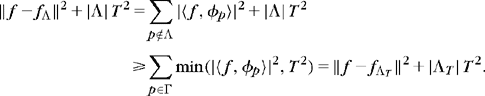
The best M-term approximation fΛ; minimizes the approximation error ‖f–fΛ‖ with |Λ| = M dictionary vectors. If D is an orthonormal basis, then Section 9.2.1 proves that the best approximation vectors are obtained by thresholding the orthogonal signal coefficients at some level T. This is not valid if D is redundant, but Theorem 12.1 proves that a best approximation is still obtained by minimizing an 10 Lagrangian where T appears as a Lagrange multiplier:
This Lagrangian penalizes the approximation error ‖f–fΛ‖2 by the number of approximation vectors.
Theorem 12.1.
is a best approximation support, which satisfies for all ![]() ,
,
Proof.
The minimization (12.3) implies that any ![]() satisfies
satisfies
Therefore, if ![]() , then
, then ![]() , which proves (12.4).
, which proves (12.4).

This theorem proves in (12.4) that minimizing the 10 Lagrangian yields a best approximation fM = fΛT of f with M = |ΛT| terms in D. The decay of the approximation error is controlled in (12.5) by the Lagrangian decay as a function of T. If D is an orthonormal basis, Theorem 12.2 derives that the resulting approximation is a thresholding at T.
NP-Hard Support Covering
In general, computing the approximation support (12.3) which minimizes the 10 Lagrangian is proved by Davis, Mallat, and Avellaneda [201] to be an NP-hard problem. This means that there exists dictionaries where finding this solution belongs to a class of NP-complete problems, for which it has been conjectured for the last 40 years that the solution cannot be found with algorithms of polynomial complexity.
The proof [201] shows that for particular dictionaries, finding a best approximation is equivalent to a set-covering problem, which is known to be NP-hard. Let us consider a simple dictionary ![]() with vectors having exactly three nonzero coordinates in an orthonormal basis
with vectors having exactly three nonzero coordinates in an orthonormal basis ![]() ,
,
If the sets ![]() define an exact partition of a subset Ω of {0,…, N – 1}, then
define an exact partition of a subset Ω of {0,…, N – 1}, then ![]() has an exact and optimal dictionary decomposition:
has an exact and optimal dictionary decomposition:
Finding such an exact decomposition for any Ω, if it exists, is an NP-hard three-sets covering problem. Indeed, the choice of one element in the solution influences the choice of all others, which essentially requires us to try all possibilities. This argument shows that redundancy makes the approximation problem much more complex. In some dictionaries such as orthonormal bases, it is possible to find optimal M-term approximations with fast algorithms, but these are particular cases.
Since optimal solutions cannot be calculated exactly, it is necessary to find algorithms of reasonable complexity that find “good” if not optimal solutions. Section 12.2 describes the search for optimal solutions restricted to sets of orthogonal vectors in well-structured tree dictionaries. Sections 12.3 and 12.4 study pursuit algorithms that search for more flexible and thus nonorthogonal sets of vectors, but that are not always optimal. Pursuit algorithms may yield optimal solutions, if the optimal support Λ satisfies exact recovery properties (studied in Section 12.5).
12.1.2 Compression by Support Coding
Chapter 10 describes transform code algorithms that quantize and code signal coefficients in an orthonormal basis. Increasing the dictionary size can reduce the approximation error by offering more choices. However, it also increases the number of bits needed to code which approximation vectors compress a signal. Optimizing the distortion rate is a trade-off between both effects.
We consider a transform code that approximates f by its orthogonal projection fΛ on the space VΛ generated by the dictionary vectors ![]() , and that quantizes the resulting coefficients. The quantization error is reduced by orthogonalizing the family
, and that quantizes the resulting coefficients. The quantization error is reduced by orthogonalizing the family ![]() , for example, with a Gram-Schmidt algorithm, which yields an orthonormal basis
, for example, with a Gram-Schmidt algorithm, which yields an orthonormal basis ![]() of VΛ. The orthogonal projection on VΛ can then be written as
of VΛ. The orthogonal projection on VΛ can then be written as
These coefficients are uniformly quantized with
and the signal recovered from quantized coefficients is
The set Λ is further restricted to coefficients ![]() , and thus
, and thus ![]() , and thus, which has no impact on
, and thus, which has no impact on ![]() .
.
Distortion Rate
Let us compute the distortion rate as a function of the dictionary size P. The compression distortion is decomposed in an approximation error plus a quantization error:
 (12.12)
With (12.11), we derive that the coding distortion is smaller than the 10 Lagrangian (12.2):
This result shows that minimizing the 10 Lagrangian reduces the compression distortion.
Having a larger dictionary offers more possibilities to choose A and further reduce the Lagrangian. Suppose that some optimization process finds an approximation support ΛT such that
where C and s depend on the dictionary design and size. The number M of nonzero quantized coefficients is ![]() . Thus, the distortion rate satisfies
. Thus, the distortion rate satisfies
where R is the total number of bits required to code the quantized coefficients of ![]() with a variable-length code.
with a variable-length code.
As in Section 10.4.1, the bit budget R is decomposed into R0 bits that code the support set ![]() , plus R1 bits to code the M nonzero quantized values Q({f, gp)) for p ∈ Λ. Let P be the dictionary size. We first code M = |ΛT| ≤ P with log2 P bits. There are
, plus R1 bits to code the M nonzero quantized values Q({f, gp)) for p ∈ Λ. Let P be the dictionary size. We first code M = |ΛT| ≤ P with log2 P bits. There are ![]() subsets of size M in a set of size P. Coding ΛT without any other prior geometric information thus requires
subsets of size M in a set of size P. Coding ΛT without any other prior geometric information thus requires ![]() bits. As in (10.48), this can be implemented with an entropy coding of the binary significance map
bits. As in (10.48), this can be implemented with an entropy coding of the binary significance map
The proportion pk of quantized coefficients of amplitude |QΔ(f, gp))| = kΔ typically has a decay of pk = (k−1+ε) for ε > 0, as in (10.57). We saw in (10.58) that coding the amplitude of the M nonzero coefficients with a logarithmic variable length lk = log2 (π2/6) + 2 log2 k, and coding their sign, requires a total number of bits R1 ~ M bits. For M ![]() P, it results that the total bit budget is dominated by the number of bits R0 to code the approximation support ΛT,
P, it results that the total bit budget is dominated by the number of bits R0 to code the approximation support ΛT,
and hence that
For a distortion satisfying (12.15), we get
When coding the approximation support ΛT in a large dictionary of size P as opposed to an orthonormal basis of size N, it introduces a factor log2 P in the distortion rate (12.17) instead of the log2N factor in (10.8). This is worth it only if it is compensated by a reduction of the approximaton constant C or an increase of the decay exponent s.
Distortion Rate for Analog Signals
A discrete signal f [n] is most often obtained with a linear discretization that projects an analog signal ![]() (x) on an approximation space UN of size N. This linear approximation error typically decays like O(N−β). From the discrete compressed signal
(x) on an approximation space UN of size N. This linear approximation error typically decays like O(N−β). From the discrete compressed signal ![]() [n], a discrete-to-analog conversion restores an analog approximation fN(x) ∈UN of
[n], a discrete-to-analog conversion restores an analog approximation fN(x) ∈UN of ![]() (x).
(x).
Let us choose a discrete resolution N~R(2s−1)/β. If the dictionary has a polynomial size P=O(Nγ), then similar to (10.62), we derive from (12.17) that
Thus, the distortion rate in a dictionary of polynomial size essentially depends on the constant C and the exponent s of the 10 Lagrangian decay ![]() in (12.14). To optimize the asymptotic distortion rate decay, one must find dictionaries of polynomial sizes that maximize s. Section 12.2.4 gives an example of a bandlet dictionary providing such optimal approximations for piecewise regular images.
in (12.14). To optimize the asymptotic distortion rate decay, one must find dictionaries of polynomial sizes that maximize s. Section 12.2.4 gives an example of a bandlet dictionary providing such optimal approximations for piecewise regular images.
12.1.3 Denoising by Support Selection in a Dictionary
A hard thresholding in an orthonormal basis is an efficient nonlinear projection estimator, if the basis defines a sparse signal approximation. Such estimators can be improved by increasing the dictionary size. A denoising estimator in a redundant dictionary also projects the observed data on a space generated by an optimized set Λ of vectors. Selecting this support is more difficult than for signal approximation or compression because the noise impacts the choice of Λ. The model selection theory proves that a nearly optimal set is estimated by minimizing the 10 Lagrangian, with an appropriate multiplier T.
Noisy signal observations are written as
where W[n] is a Gaussian white noise of variance σ2. Let ![]() be a dictionary of P-unit norm vectors. To any subfamily of vectors,
be a dictionary of P-unit norm vectors. To any subfamily of vectors, ![]() corresponds an orthogonal projection estimator on the space VΛ generated by these vectors:
corresponds an orthogonal projection estimator on the space VΛ generated by these vectors:
The orthogonal projection in VΛ satisfies ![]() , so
, so
The bias term ‖f–f‖2 is the signal approximation error, which decreases when |Λ| increases. On the contrary, the noise energy ‖WΛ‖2 in VΛ increases when |Λ| increases. Reducing the risk amounts to finding a projection support A that balances these two terms to minimize their sum.
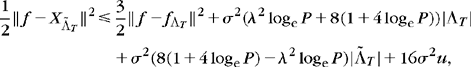
Since VΛ is a space of dimension |Λ|, the projection of a white noise of variance σ2 satisfies E{‖WΛ‖2} = |Λ| σ2. However, there are 2P possible subsets Λ in Γ, and ‖WΛ;‖2 may potentially take much larger values than |Λ|σ2 for some particular sets Λ. A concentration inequality proved in Lemma 12.1 of Theorem 12.3 shows that for any subset Λ of Γ,
with a probability that tends to 1 as P increases for Λ large enough. It results that the estimation error is bounded by the approximation Lagrangian:
However, the set ΛT that minimizes this Lagrangian,
can only be found by an oracle because it depends on f, which is unknown. Thus, we need to find an estimator that is nearly as efficient as the oracle projector on this subset ΛT of vectors.
Penalized Empirical Error
Estimating the oracle set ΛT in (12.21) requires us to estimate ‖f−fΛ‖2 for any Λ ⊂ Γ. A crude estimator is given by the empirical norm
This may seem naive because it yields a large error,
Since X = f + W and ![]() , the expected error is
, the expected error is
which is of the order of Nσ2 if |Λ| ![]() N. However, the first large term does not influence the choice of Λ. The component that depends on Λ is the smaller term
N. However, the first large term does not influence the choice of Λ. The component that depends on Λ is the smaller term ![]() , which is only of the order |Λ|σ2.
, which is only of the order |Λ|σ2.
Thus, we estimate ![]() with
with ![]() in the oracle formula (12.21), and define the best empirical estimation
in the oracle formula (12.21), and define the best empirical estimation ![]() as the orthogonal projection on a space
as the orthogonal projection on a space ![]() , where
, where ![]() minimizes the penalized empirical risk:
minimizes the penalized empirical risk:
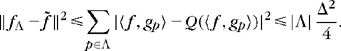
Theorem 12.3 proves that this estimated set ![]() yields a risk that is within a factor of 4 of the risk obtained by the oracle set ΛT in (12.21). This theorem is a consequence of the more general model selection theory of Barron, Birge, and Massart [97], where the optimization of Λ is interpreted as a model selection. Theorem 12.3 was also proved by Donoho and Johnstone [220] for estimating a best basis in a dictionary of orthonormal bases.
yields a risk that is within a factor of 4 of the risk obtained by the oracle set ΛT in (12.21). This theorem is a consequence of the more general model selection theory of Barron, Birge, and Massart [97], where the optimization of Λ is interpreted as a model selection. Theorem 12.3 was also proved by Donoho and Johnstone [220] for estimating a best basis in a dictionary of orthonormal bases.
Theorem 12.3: Barron, Birgé, Massart, Donoho, Johnstone. Let σ2 be the noise variance and ![]() with
with ![]() . For any f ∈
. For any f ∈ ![]() N, the best empirical set
N, the best empirical set
yields a projection estimator ![]() of f, which satisfies
of f, which satisfies
Proof.
Concentration inequalities are at the core of this result. Indeed, the penalty T2 |Λ| must dominate the random fluctuations of the projected noise. We give a simplified proof provided in [233]. Lemma 12.1 uses a concentration inequality for Gaussian variables to ensure with high probability that the noise energy is simultaneously small in all the subspaces VΛ spanned by subsets of vectors in D.
Lemma 12.1.
with a probability greater than 1−2e−u/P.
This lemma is based on Tsirelson’s lemma which proves that for any function L from ![]() N to
N to ![]() that is 1-Lipschitz (|L(f)−L(g)| ≤ ‖f−g‖), and for any normalized Gaussian white noise vector W of variance σ2 = 1,
that is 1-Lipschitz (|L(f)−L(g)| ≤ ‖f−g‖), and for any normalized Gaussian white noise vector W of variance σ2 = 1,
The orthogonal projection’s norm L(W) = ‖WΛ;‖ is 1-Lipschitz. Applying Tsirelson’s lemma to ![]() for
for ![]() yields
yields
Let us now compute the probability of the existence of a set ![]() that does not satisfy the lemma condition (12.25), by considering each subset of Γ:
that does not satisfy the lemma condition (12.25), by considering each subset of Γ:

from which we get (12.25) by observing that ![]() because
because ![]() . This finishes the proof of Lemma 12.1.
. This finishes the proof of Lemma 12.1.
By construction, the best empirical set ![]() compared to the oracle set ΛT in (12.21) satisfies
compared to the oracle set ΛT in (12.21) satisfies
By using ![]() and a similar equality for
and a similar equality for ![]() together with the equalities
together with the equalities ![]() and
and ![]() , we derive that
, we derive that
The vectors ![]() generate a space
generate a space ![]() of dimension smaller or equal to
of dimension smaller or equal to ![]() . We denote by
. We denote by ![]() the orthogonal projection of the noise W on this space. The inner product is bounded by writing
the orthogonal projection of the noise W on this space. The inner product is bounded by writing
Lemma 12.1 implies
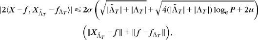
with a probability greater than ![]() . Applying
. Applying ![]() successively with β = 1/2 and β = 1 gives
successively with β = 1/2 and β = 1 gives

Inserting this bound in (12.26) yields
So that if ![]() ,
,
which implies for ![]() that
that
where this result holds with probability greater than ![]() .
.
Since this is valid for all u ≤ 0, one has
which implies by integration over u that
which proves the theorem result (12.24).
This theorem proves that the selection of a best-penalized empirical projection produces a risk that is within a factor of 4 of the minimal oracle risk obtained by selecting the best dictionary vectors that approximate f. Birge and Massart [114] obtain a better lower bound for Λ (roughly ![]() and thus
and thus ![]() ) and a multiplicative factor smaller than 4 with a more complex proof using Talgrand’s concentration inequalities.
) and a multiplicative factor smaller than 4 with a more complex proof using Talgrand’s concentration inequalities.
If D is an orthonormal basis, then Theorem 12.2 proves that the optimal estimator ![]() is a hard-thresholding estimator at T. Thus, this theorem generalizes the thresholding estimation theorem (11.7) of Donoho and Johnstone that computes an upper bound of the thresholding risk in an orthonormal basis with P = N.
is a hard-thresholding estimator at T. Thus, this theorem generalizes the thresholding estimation theorem (11.7) of Donoho and Johnstone that computes an upper bound of the thresholding risk in an orthonormal basis with P = N.
The minimum Lagrangian value L0(T, f, ΛT) is reduced by increasing the size of the dictionary D. However, this is paid by also increasing T proportionally to logeP, so that the penalization term T2|Λ| is big enough to dominate the impact of the noise on the selection of dictionary vectors. Increasing D is thus worth it only if the decay of L0(T, f, ΛT) compensates the increase of T, as in the compression application of Section 12.1.2.
Estimation Risk for Analog Signals
Discrete signals are most often obtained by discretizing analog signals, and the estimation risk can also be computed on the input analog signal, as in Section 11.5.3. Let f[n] be the discrete signal obtained by approximating an analog signal f(x) in an approximation space UN of size N. An estimator ![]() of f[n] is converted into an analog estimation F(x) ∈ UN of f(x), with a discrete-to-analog conversion. We verify as in (11.141) that the total risk is the sum of the discrete estimation risk plus a linear approximaton error:
of f[n] is converted into an analog estimation F(x) ∈ UN of f(x), with a discrete-to-analog conversion. We verify as in (11.141) that the total risk is the sum of the discrete estimation risk plus a linear approximaton error:
Suppose that the dictionary has a polynomial size P = O(Nγ) and that the 10 Lagrangian decay satisfies
If the linear approximation error satisfies ![]() , then by choosing
, then by choosing ![]() , we derive from (12.24) in Theorem 12.3 that
, we derive from (12.24) in Theorem 12.3 that
When the noise variance σ2 decreases, the risk decay depends on the decay exponent s of the 10 Lagrangian. Optimized dictionaries should thus increase s as much as possible for any given class Θ of signals.
12.2 DICTIONARIES OF ORTHONORMAL BASES
To reduce the complexity of sparse approximations selected in a redundant dictionary, this section restricts such approximations to families of orthogonal vectors. Eliminating approximations from nonorthogonal vectors reduces the number of possible approximation sets Λ in D, which simplifies the optimization. In an orthonormal basis, an optimal nonlinear approximation selects the largest-amplitude coefficients. Dictionaries of orthonormal bases take advantage of this property by regrouping orthogonal dictionary vectors in a multitude of orthonormal bases.
Definition 12.1. A dictionary D is said to be a dictionary of orthonormal bases of ![]() N if any family of orthogonal vectors in D also belongs to an orthonormal basis B of
N if any family of orthogonal vectors in D also belongs to an orthonormal basis B of ![]() N included in D.
N included in D.
A dictionary of orthonormal bases ![]() is thus a family of P>N vectors that can also be viewed as a union of orthonormal bases, many of which share common vectors. Wavelet packets and local cosine bases in Chapter 8 define dictionaries of orthonormal bases. In Section 12.2.1 we prove that finding a best signal approximation with orthogonal dictionary vectors can be casted as a search for a best orthonormal basis in which orthogonal vectors are selected by a thresholding. Compression and denoising algorithms are implemented in such a best basis. Tree-structured dictionaries are introduced in Section 12.2.2, in order to compute best bases with a fast dynamic programming algorithm.
is thus a family of P>N vectors that can also be viewed as a union of orthonormal bases, many of which share common vectors. Wavelet packets and local cosine bases in Chapter 8 define dictionaries of orthonormal bases. In Section 12.2.1 we prove that finding a best signal approximation with orthogonal dictionary vectors can be casted as a search for a best orthonormal basis in which orthogonal vectors are selected by a thresholding. Compression and denoising algorithms are implemented in such a best basis. Tree-structured dictionaries are introduced in Section 12.2.2, in order to compute best bases with a fast dynamic programming algorithm.
12.2.1 Approximation, Compression, and Denoising in a Best Basis
Sparse approximations of signals f ∈ ![]() N are constructed with orthogonal vectors selected from a dictionary
N are constructed with orthogonal vectors selected from a dictionary ![]() of orthonormal bases with compression and denoising applications.
of orthonormal bases with compression and denoising applications.
Best Basis
We denote by Λo ⊂ γ a collection of orthonormal vectors in D. Sets of nonorthogonal vectors are not considered. The orthogonal projection of f on the space generated by these vectors is then ![]() .
.
In an orthonormal basis ![]() , Theorem 12.2 proves that the Lagrangian
, Theorem 12.2 proves that the Lagrangian ![]() is minimized by selecting coefficients above T. The resulting minimum is
is minimized by selecting coefficients above T. The resulting minimum is
Theorem 12.4 derives that a best approximation from orthogonal vectors in D is obtained by thresholding coefficients in a best basis that minimizes this 10 Lagrangian.
Theorem 12.4.
the thresholded set ![]() satisfies
satisfies
and for all Λo ⊂ γ,
Proof.
Since any vector in D belongs to an orthonormal basis B ⊂ D, we can write ![]() , so (12.28) with (12.29) implies (12.30). The optimal approximation result (12.31), like (12.4), comes from the fact that
, so (12.28) with (12.29) implies (12.30). The optimal approximation result (12.31), like (12.4), comes from the fact that ![]() .
.
This theorem proves in (12.31) that the thresholding approximation ![]() of f in the best orthonormal basis BT is the best approximation of f from M = |ΛT| orthogonal vectors in D.
of f in the best orthonormal basis BT is the best approximation of f from M = |ΛT| orthogonal vectors in D.
Compression in a Best Orthonormal Basis
Section 12.1.2 shows that quantizing signal coefficients over orthogonal dictionary vectors ![]() yields a distortion
yields a distortion
where 2T = Δ is the quantization step. A best transform code that minimizes this Lagrangian upper bound is thus implemented in the best orthonormal basis ![]() T in (12.29).
T in (12.29).
With an entropy coding of the significance map (12.16), the number of bits R0 to code the indexes of the M nonzero quantized coefficients among P dictionary elements is ![]() . However, the number of sets Λo of orthogonal vectors in D is typically much smaller than the number 2P of subsets Λ in γ and the resulting number R0 of bits is thus smaller.
. However, the number of sets Λo of orthogonal vectors in D is typically much smaller than the number 2P of subsets Λ in γ and the resulting number R0 of bits is thus smaller.
A best-basis search improves the distortion rate d(R, f) if the Lagrangian approximation reduction is not compensated by the increase of R0 due to the increase of the number of orthogonal vector sets. For example, if the original signal is piecewise smooth, then a best wavelet packet basis does not concentrate the signal energy much more efficiently than a wavelet basis. Despite the fact that a wavelet packet dictionary includes a wavelet basis, the distortion rate in a best wavelet packet basis is then larger than in a single wavelet basis. For geometrically regular images, Section 12.2.4 shows that a dictionary of bandlet orthonormal bases reduces the distortion rate of a wavelet basis.
Denoising in a Best Orthonormal Basis
To estimate a signal f from noisy signal observations
where W[n] is a Gaussian white noise, Theorem 12.3 proves that a nearly optimal estimator is obtained by minimizing a penalized empirical Lagrangian,
Restricting Λ to be a set Λo of orthogonal vectors in ![]() reduces the set of possible signal models. As a consequence, Theorem 12.3 remains valid for this subfamily of models. Theorem 12.4 proves in (12.30) that the Lagrangian (12.32) is minimized by thresholding coefficients in a best basis. A best-basis thresholding thus yields a risk that is within a factor of 4 of the best estimation obtained by an oracle. This best basis can be calculated with a fast algorithm described in Section 12.2.2.
reduces the set of possible signal models. As a consequence, Theorem 12.3 remains valid for this subfamily of models. Theorem 12.4 proves in (12.30) that the Lagrangian (12.32) is minimized by thresholding coefficients in a best basis. A best-basis thresholding thus yields a risk that is within a factor of 4 of the best estimation obtained by an oracle. This best basis can be calculated with a fast algorithm described in Section 12.2.2.
12.2.2 Fast Best-Basis Search in Tree Dictionaries
Tree dictionaries of orthonormal bases are constructed with a recursive split of orthogonal vector spaces and by defining specific orthonormal bases in each subspace. For any additive cost function such as the 10 Lagrangian (12.2), a fast dynamic programming algorithm finds a best basis with a number of operations proportional to the size P of the dictionary.
Recursive Split of Vectors Spaces
A tree dictionary ![]() is obtained by recursively dividing vector spaces into q orthogonal subspaces, up to a maximum recursive depth. This recursive split is represented by a tree. A vector space Wld is associated to each tree node at a depth d and position l. The q children of this node correspond to an orthogonal partition of Wld into q orthogonal subspaces
is obtained by recursively dividing vector spaces into q orthogonal subspaces, up to a maximum recursive depth. This recursive split is represented by a tree. A vector space Wld is associated to each tree node at a depth d and position l. The q children of this node correspond to an orthogonal partition of Wld into q orthogonal subspaces ![]() at depth d + 1, located at the positions ql+iO≤i<q:
at depth d + 1, located at the positions ql+iO≤i<q:
 (12.33)
Space ![]() at the root of the tree is the full signal space
at the root of the tree is the full signal space ![]() N. One or several specific orthonormal bases are constructed for each space Wld. The dictionary D is the union of all these specific orthonormal bases for all the spaces Wld of the tree.
N. One or several specific orthonormal bases are constructed for each space Wld. The dictionary D is the union of all these specific orthonormal bases for all the spaces Wld of the tree.
Chapter 8 defines dictionaries of wavelet packet and local cosine bases along binary trees (q = 2) for one-dimensional signals and along quad-trees (q = 4) for images. These dictionaries are constructed with a single basis for each space Wld. For signals of size N, they have P = N log2 N vectors. The bandlet dictionary in Section 12.2.4 is also defined along a quad-tree, but each space Wld has several specific orthonormal bases corresponding to different image geometries.
An admissible subtree of a full dictionary tree is a subtree where each node is either a leaf or has its q children. Figure 12.1(b) gives an example of a binary admissible tree. We verify by induction that the vector spaces at the leaves of an admissible tree define an orthogonal partition of W00 = ![]() N into orthogonal subspaces. The union of orthonormal bases of these spaces is therefore an orthonormal basis of
N into orthogonal subspaces. The union of orthonormal bases of these spaces is therefore an orthonormal basis of ![]() N.
N.

Additive Costs
A best basis can be defined with a cost function that is not necessarily the 10 Lagrangian (12.2). An additive cost function of a signal f in a basis ![]() is defined as a sum of independent contributions from each coefficient in
is defined as a sum of independent contributions from each coefficient in ![]() :
:
A best basis of ![]() N in
N in ![]() minimizes the resulting cost,
minimizes the resulting cost,
The 10 Lagrangian (12.2) is an example of additive cost function,
The minimization of an 11 norm is obtained with
In Section 12.4.1 we introduce a basis pursuit algorithm that also minimizes the 11 norm of signal coefficients in a redundant dictionary. A basis pursuit selects a best basis but without imposing any orthogonal constraint.
Fast Best-Basis Selection
The fast best-basis search algorithm, introduced by Coifman and Wickerhauser [180], relies on the dictionary tree structure and on the cost additivity. This algorithm is a particular instance of the Classification and Regression Tree (CART) algorithm by Breiman et al. [9]. It explores all tree nodes, from bottom to top, and at each node it computes the best basis ![]() of the corresponding space Wld.
of the corresponding space Wld.
The cost additivity property (12.34) implies that an orthonormal basis ![]() , which is a union of q orthonormal families Bi, has a cost equal to the sum of their cost:
, which is a union of q orthonormal families Bi, has a cost equal to the sum of their cost:

As a result, the best basis ![]() , which minimizes this cost among all bases of
, which minimizes this cost among all bases of ![]() , is either one of the specific bases of
, is either one of the specific bases of ![]() or a union of the best bases
or a union of the best bases ![]() that were previously calculated for each of its subspace
that were previously calculated for each of its subspace ![]() for 0 ≤ i<q. The decision is thus performed by minimizing the resulting cost, as described in Algorithm 12.1.
for 0 ≤ i<q. The decision is thus performed by minimizing the resulting cost, as described in Algorithm 12.1.
ALGORITHM 12.1
![]() Compute all dictionary coefficients
Compute all dictionary coefficients ![]() .
.
![]() Initialize the cost of each tree space
Initialize the cost of each tree space ![]() by finding the basis
by finding the basis ![]() of minimum cost among all specific bases
of minimum cost among all specific bases ![]() of
of ![]() :
:
![]() For each tree node (d,l), visited from the bottom to the top (d decreasing), if we are not at the bottom and if
For each tree node (d,l), visited from the bottom to the top (d decreasing), if we are not at the bottom and if

then set ![]() ; otherwise set
; otherwise set ![]() .
.
This algorithm outputs the best basis ![]() that has a minimum cost among all bases of the dictionary. For wavelet packet and local cosine dictionaries, there is a single specific basis per space
that has a minimum cost among all bases of the dictionary. For wavelet packet and local cosine dictionaries, there is a single specific basis per space ![]() , so (12.38) is reduced to computing the cost in this basis. In a bandlet dictionary there are many specific bases for each
, so (12.38) is reduced to computing the cost in this basis. In a bandlet dictionary there are many specific bases for each ![]() corresponding to different geometric image models.
corresponding to different geometric image models.
For a dictionary of size P, the number of comparisons and additions to construct this best basis is O(P). The algorithmic complexity is thus dominated by the computation of the P dictionary coefficients ![]() . If implemented with O(P) operations with a fast transform, then the overall computational algorithmic complexity is O(P). This is the case for wavelet packet, local cosine, and bandlet dictionaries.
. If implemented with O(P) operations with a fast transform, then the overall computational algorithmic complexity is O(P). This is the case for wavelet packet, local cosine, and bandlet dictionaries.
12.2.3 Wavelet Packet and Local Cosine Best Bases
A best wavelet packet or local cosine basis selects time-frequency atoms that match the time-frequency resolution of signal structures. Therefore, it adapts the time-frequency geometry of the approximation support ΛT. Wavelet packet and local cosine dictionaries are constructed in Chapter 8. We evaluate these approximations through examples that also reveal their limitations.
Best Orthogonal Wavelet Packet Approximations
A wavelet packet orthogonal basis divides the frequency axis into intervals of varying dyadic sizes 2. Each frequency interval is covered by a wavelet packet function that is uniformly translated in time. A best wavelet packet basis can thus be interpreted as a “best” segmentation of the frequency axis in dyadic sizes intervals.
A signal is well approximated by a best wavelet packet basis, if in any frequency interval, the high-energy structures have a similar time-frequency spread. The time translation of the wavelet packet that covers this frequency interval is then well adapted to approximating all the signal structures in this frequency range that appear at different times. In the best basis computed by minimizing the 10 Lagrangian in (12.36), Theorem 12.4 proves that the set of ΛT of wavelet packet coefficients above T correspond to the orthogonal wavelet packet vectors that best approximate f in the whole wavelet packet dictionary. These wavelet packets are represented by Heisenberg boxes, as explained in Section 8.1.2.
Figure 12.2 gives the best wavelet packet approximation set ΛT of a signal composed of two hyperbolic chirps. The proportion of wavelet packet coefficients that are retained is M/N = |ΛT|/N = 8%. The resulting best M-term orthogonal approximaton ![]() has a relative error
has a relative error ![]() . The wavelet packet tree was calculated with the symmlet 8 conjugate mirror filter. The time support of chosen wavelet packets is reduced at high frequencies to adapt itself to the chirps’ rapid modification of frequency content. The energy distribution revealed by the wavelet packet Heisenberg boxes in ΛT is similar to the scalogram calculated in Figure 4.17.
. The wavelet packet tree was calculated with the symmlet 8 conjugate mirror filter. The time support of chosen wavelet packets is reduced at high frequencies to adapt itself to the chirps’ rapid modification of frequency content. The energy distribution revealed by the wavelet packet Heisenberg boxes in ΛT is similar to the scalogram calculated in Figure 4.17.
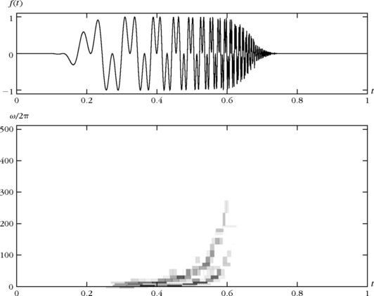
FIGURE 12.2 The top signal includes two hyperbolic chirps. The Heisenberg boxes of the best orthogonal wavelet packets in ΛT are shown in the bottom image. The darkness of each rectangle is proportional to the amplitude of the corresponding wavelet packet coefficient.
Figure 8.6 gives another example of a best wavelet packet basis for a different multichirp signal, calculated with the entropy cost C(x) = |x| loge |x| in (12.34).
Let us mention that the application of best wavelet packet bases to pattern recognition is difficult because these dictionaries are not translation invariant. If the signal is translated, its wavelet packet coefficients are severely modified and the Lagrangian minimization may yield a different basis. This remark applies to local cosine bases as well.
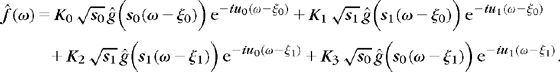
If the signal includes different types of high-energy structures, located at different times but in the same frequency interval, there is no wavelet packet basis that is well adapted to all of them. Consider, for example, a sum of four transients centered, respectively, at u0 and u1 at two different frequencies ζ0 and ζ1:
 (12.39)
The smooth window g has a Fourier transform g whose energy is concentrated at low frequencies. The Fourier transform of the four transients have their energy concentrated in frequency bands centered, respectively, at ζ0 and ζ1:
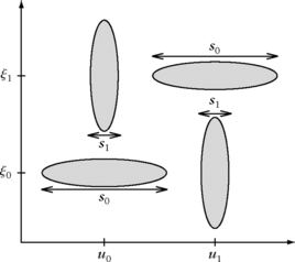
If s0 and s1 have different values, the time and frequency spread of these transients is different, which is illustrated in Figure 12.3. In the best wavelet packet basis selection, the first transient ![]() “votes” for a wavelet packet basis with a scale 2j that is of the order s0 at the frequency ζ0 whereas
“votes” for a wavelet packet basis with a scale 2j that is of the order s0 at the frequency ζ0 whereas ![]() “votes” for a wavelet packet basis with a scale 2j that is close to s1 at the same frequency. The “best” wavelet packet is adapted to the transient of highest energy. The energy of the smaller transient is then spread across many “best” wavelet packets. The same thing happens for the second pair of transients located in the frequency neighborhood of ξ1.
“votes” for a wavelet packet basis with a scale 2j that is close to s1 at the same frequency. The “best” wavelet packet is adapted to the transient of highest energy. The energy of the smaller transient is then spread across many “best” wavelet packets. The same thing happens for the second pair of transients located in the frequency neighborhood of ξ1.
Speech recordings are examples of signals that have properties that rapidly change in time. At two different instants in the same frequency neighborhood, the signal may have totally different energy distributions. A best orthogonal wavelet packet basis is not adapted to this time variation and gives poor nonlinear approximations. Sections 12.3 and 12.4 show that a more flexible nonorthogonal approximation with wavelet packets, computed with a pursuit algorithm, can have the required flexibility.
As in one dimension, an image is well approximated in a best wavelet packet basis if its structures within a given frequency band have similar properties across the whole image. For natural scene images, a best wavelet packet often does not provide much better nonlinear approximations than the wavelet basis included in this wavelet packet dictionary. However, for specific classes of images such as fingerprints, one may find wavelet packet bases that significantly outperform the wavelet basis [122].
Best Orthogonal Local Cosine Representations
Tree dictionaries of local cosine bases are constructed in Section 8.5 with P = N log2 N local cosine vectors. They divide the time axis into intervals of varying dyadic sizes. A best local cosine basis adapts the time segmentation to the variations of the signal time-frequency structures. It is computed with O(Nlog2N) operations with the best-basis search algorithm from Section 12.2.2.
In comparison with wavelet packets, we gain time adaptation but we lose frequency flexibility. A best local cosine basis is therefore well adapted to approximating signals with properties that may vary in time, but that do not include structures of very different time and frequency spreads at any given time. Figure 12.4 shows the Heisenberg boxes of the set ΛT of orthogonal local cosine vectors that best approximate the recording of a bird song, computed by minimizing the 10 Lagrangian (12.36). The chosen threshold T yields a relative approximation error ![]() with |ΛT|/N = 11% coefficients. The selected local cosine vectors have a time and frequency resolution adapted to the transients and harmonic structures of the signal. Figure 8.19 shows a best local cosine basis that is calculated with an entropy cost function for a speech recording.
with |ΛT|/N = 11% coefficients. The selected local cosine vectors have a time and frequency resolution adapted to the transients and harmonic structures of the signal. Figure 8.19 shows a best local cosine basis that is calculated with an entropy cost function for a speech recording.
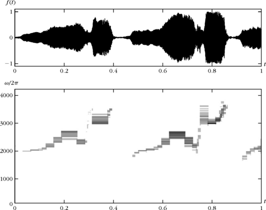
FIGURE 12.4 Recording of a bird song (top). The Heisenberg boxes of the best orthogonal local cosine vectors in ΛT are shown in the bottom image. The darkness of each rectangle is proportional to the amplitude of the local cosine coefficient.
The sum of four transients (12.39) is not efficiently represented in a wavelet packet basis but neither is it well approximated in a best local cosine basis. Indeed, if the scales s0 and s1 are very different, at u0 and u1 this signal includes two transients at the frequency ζ0 and ζ1, respectively, that have a very different time-frequency spread. In each time neighborhood, the size of the window is adapted to the transient of highest energy. The energy of the second transient is spread across many local cosine vectors. Efficient approximations of such signals require more flexibility, which is provided by the pursuit algorithms from Sections 12.3 and 12.4. Figure 12.5 gives a denoising example with a best local cosine estimator. The signal in Figure 12.5(b) is the bird song contaminated by an additive Gaussian white noise of variance σ2 with an SNR of 12 db. According to Theorem 12.3, a best orthogonal projection estimator is computed by selecting a set ![]() of best orthogonal local cosine dictionary vectors, which minimizes an empirical penalized risk. This penalized risk corresponds to the empirical 10 Lagrangian (12.23), which is minimized by the best-basis algorithm. The chosen threshold of T = 3.5 σ is well below the theoretical universal threshold of
of best orthogonal local cosine dictionary vectors, which minimizes an empirical penalized risk. This penalized risk corresponds to the empirical 10 Lagrangian (12.23), which is minimized by the best-basis algorithm. The chosen threshold of T = 3.5 σ is well below the theoretical universal threshold of ![]() , which improves the SNR. The Heisenberg boxes of local cosine vectors indexed by
, which improves the SNR. The Heisenberg boxes of local cosine vectors indexed by ![]() are shown in boxes of the remaining coefficients in Figure 12.5(c). The orthogonal projection
are shown in boxes of the remaining coefficients in Figure 12.5(c). The orthogonal projection ![]() is shown in Figure 12.5(d).
is shown in Figure 12.5(d).

FIGURE 12.5 (a) Original bird song. (b) Noisy signal (SNR = 12 db). (c) Heisenberg boxes of the set ![]() of estimated best orthogonal local cosine vectors. (d) Estimation reconstructed from noisy local cosine coefficients in
of estimated best orthogonal local cosine vectors. (d) Estimation reconstructed from noisy local cosine coefficients in ![]() (SNR = 15.5db).
(SNR = 15.5db).
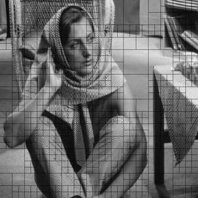
In two dimensions, a best local cosine basis divides an image into square windows that have a size adapted to the spatial variations of local image structures. Figure 12.6 shows the best-basis segmentation of the Barbara image, computed by minimizing the 11 norm of its coefficients, with the 11 cost function (12.37). The squares are bigger in regions where the image structures remain nearly the same. Figure 8.22 shows another example of image segmentation with a best local cosine basis, also computed with an 11 norm.
12.2.4 Bandlets for Geometric Image Regularity
Bandlet dictionaries are constructed to improve image representations by taking advantage of their geometric regularity. Wavelet coefficients are not optimally sparse but inherit geometric image regularity. A bandlet transform applies a directional wavelet transform over wavelet coefficients to reduce the number of large coefficients. This directional transformation depends on a geometric approximation model calculated from the image. Le Pennec, Mallat, and Peyre [342, 365, 396] introduced dictionaries of orthogonal bandlet bases, where the best-basis selection optimizes the geometric approximation model. For piecewise Cα images, the resulting M-term bandlet approximations have an optimal asymptotic decay in O(M−α).
Approximation of Piecewise Cα Images
Definition 9.1 defines a piecewise Cα image f as a function that is uniformly Lipschitz α everywhere outside a set of edge curves, which are also uniformly Lipschitz α. This image may also be blurred by an unknown convolution kernel. If f is uniformly Lipschitz α without edges, then Theorem 9.16 proves that a linear wavelet approximation has an optimal error decay ![]() . Edges produce a larger linear approximation error
. Edges produce a larger linear approximation error ![]() , which is improved by a nonlinear wavelet approximation
, which is improved by a nonlinear wavelet approximation ![]() , but without recovering the O(M−α) decay. For α = 2, Section 93 shows that a piecewise linear approximation over an optimized adaptive triangulation with M triangles reaches the error decay O(M−2). Thresholding curvelet frame coefficients also yields a nonlinear approximation error
, but without recovering the O(M−α) decay. For α = 2, Section 93 shows that a piecewise linear approximation over an optimized adaptive triangulation with M triangles reaches the error decay O(M−2). Thresholding curvelet frame coefficients also yields a nonlinear approximation error ![]() that is nearly optimal. However, curvelet approximations are not as efficient as wavelets for less regular functions such as bounded variation images. If f is piecewise Cα with α > 2, curvelets cannot improve the M−2 decay either.
that is nearly optimal. However, curvelet approximations are not as efficient as wavelets for less regular functions such as bounded variation images. If f is piecewise Cα with α > 2, curvelets cannot improve the M−2 decay either.
The beauty of wavelet and curvelet approximation comes from their simplicity. A simple thresholding directly selects the signal approximation support. However, for images with geometric structures of various regularity, these approximations do not remain optimal when the regularity exponent α changes. It does not seem possible to achieve this result without using a redundant dictionary, which requires a more sophisticated approximation scheme.
Elegant adaptive approximation schemes in redundant dictionaries have been developed for images having some geometric regularity. Several algorithms are based on the lifting technique described in Section 7.8, with lifting coefficients that depend on the estimated image regularity [155, 234, 296, 373, 477]. The image can also be segmented adaptively in dyadic squares of various sizes, and approximated on each square by a finite element such as a wedglet, which is a step edge along a straight line with an orientation that is adjusted [216]. Refinements with polynomial edges have also been studied [436], but these algorithms do not provide M-term approximation errors that decay like O(M−α) for all piecewise regular Cα images.
Bandletization of Wavelet Coefficients
A bandlet transform takes advantage of the geometric regularity captured by a wavelet transform. The decomposition coefficients of f in an orthogonal wavelet basis can be written as
for x = (x1, x2) and n = (n1, n2). The function ![]() has the directional regularity of f, for example along an edge, and it is regularized by the convolution with
has the directional regularity of f, for example along an edge, and it is regularized by the convolution with ![]() . Figure 12.7 shows a zoom on wavelet coefficients near an edge.
. Figure 12.7 shows a zoom on wavelet coefficients near an edge.

FIGURE 12.7 Orthogonal wavelet coefficients at a scale 2j are samples of a function ![]() , shown in (a). The filtered image
, shown in (a). The filtered image ![]() varies regularly when moving along an edge γ (b).
varies regularly when moving along an edge γ (b).
Bandlets retransform wavelet coefficients to take advantage of their directional regularity. This is implemented with a directional wavelet transform applied over wavelet coefficients, which creates new vanishing moments in appropriate directions. The resulting bandlets are written as
where ![]() is a directional wavelet of length 2i, of width 2l, and that has a position indexed by m in the wavelet coefficient array. The bandlet function
is a directional wavelet of length 2i, of width 2l, and that has a position indexed by m in the wavelet coefficient array. The bandlet function ![]() is a finite linear combination of wavelets
is a finite linear combination of wavelets ![]() and thus has the same regularity as these wavelets. Since
and thus has the same regularity as these wavelets. Since ![]() has a square support of width proportional to 2j, the bandlet φp has a support length proportional to 2j+i and a support width proportional to 2j.
has a square support of width proportional to 2j, the bandlet φp has a support length proportional to 2j+i and a support width proportional to 2j.
If the regularity exponent α is known then in a neighborhood of an edge, one would like to have elongated bandlets with an aspect ratio defined by 2l+j = (2i+j)α, and thus l = αi + (a − 1)j. Curvelets satisfy this property for α = 2. However, when α is not known in advance and may change, the scale parameters i and l must be adjusted adaptively.
As a result of (12.41), the bandlet coefficients of a signal ![]() can be written as
can be written as
They are computed by applying a discrete directional wavelet tranform on the signal wavelet coefficients ![]() for each k and 2j. This is also a called a bandletization of wavelet coefficients.
for each k and 2j. This is also a called a bandletization of wavelet coefficients.
Geometric Approximation Model
The discrete directional wavelets ![]() are defined with a geometric approximation model providing information about the directional image regularity. Many constructions are possible [359]. We describe here a geometric approximation model that is piecewise parallel and yields orthogonal bandlet bases.
are defined with a geometric approximation model providing information about the directional image regularity. Many constructions are possible [359]. We describe here a geometric approximation model that is piecewise parallel and yields orthogonal bandlet bases.
For each scale 2j and direction k, the array of wavelet transform coefficients ![]() is divided into squares of various sizes, as shown in Figure 12.8(b). In regular image regions, wavelet coefficients are small and do not need to be retransformed. Near junctions, the image is irregular in all directions and these few wavelet coefficients are not retransformed either. It is in the neighborhood of edges and directional image structures that an appropriate retransformation can improve the wavelet sparsity.
is divided into squares of various sizes, as shown in Figure 12.8(b). In regular image regions, wavelet coefficients are small and do not need to be retransformed. Near junctions, the image is irregular in all directions and these few wavelet coefficients are not retransformed either. It is in the neighborhood of edges and directional image structures that an appropriate retransformation can improve the wavelet sparsity.

FIGURE 12.8 (a) Wavelet coefficients of the image. (b) Example of segmentation of an array of wavelet coefficients ![]() for a particular direction k and scale 2j.
for a particular direction k and scale 2j.
A geometric flow is defined over each edge square. It provides the direction along which the discrete bandlets ![]() are constructed. It is a vector field, which is parallel horizontally or vertically and points in local directions in which
are constructed. It is a vector field, which is parallel horizontally or vertically and points in local directions in which ![]() is the most regular. Figure 12.9(a) gives an example. The segmentation of wavelet coefficients in squares and the specification of a geometric flow in each square defines a geometric approximation model that is used to construct a bandlet basis.
is the most regular. Figure 12.9(a) gives an example. The segmentation of wavelet coefficients in squares and the specification of a geometric flow in each square defines a geometric approximation model that is used to construct a bandlet basis.

FIGURE 12.9 (a) Square of wavelet coefficients including an edge. A geometric flow nearly parallel to the edge is shown with arrows. (b) A vertical warping w maps the flow onto a horizontal flow. (c) Support of directional wavelets ![]() of length 2i and width 2l in the warped domain. (d) Directional wavelets
of length 2i and width 2l in the warped domain. (d) Directional wavelets ![]() in the square of wavelet coefficients.
in the square of wavelet coefficients.
Bandlets with Alpert Wavelets
Let us consider a square of wavelet coefficients where a geometric flow is defined. We suppose that the flow is parallel vertically. Its vectors can thus be written ![]() . Let
. Let ![]() be a primitive of
be a primitive of ![]() . Wavelet coefficients are translated vertically with a warping operator
. Wavelet coefficients are translated vertically with a warping operator ![]() so that the resulting geometric flow becomes horizontal, as shown in Figure 12.9(b). In the warped domain, the regularity of
so that the resulting geometric flow becomes horizontal, as shown in Figure 12.9(b). In the warped domain, the regularity of ![]() is now horizontal.
is now horizontal.
Warped directional wavelets ![]() are defined to take advantage of this horizontal regularity over the translated orthogonal wavelet coefficients, which are not located on a square grid anymore. Directional wavelets can be constructed with piecewise polynomial Alpert wavelets [84], which are adapted to nonuniform sampling grids [365] and have q vanishing moments. Over a square of width 2i, a discrete Alpert wavelet
are defined to take advantage of this horizontal regularity over the translated orthogonal wavelet coefficients, which are not located on a square grid anymore. Directional wavelets can be constructed with piecewise polynomial Alpert wavelets [84], which are adapted to nonuniform sampling grids [365] and have q vanishing moments. Over a square of width 2i, a discrete Alpert wavelet ![]() has a length 2i, a total of 2i × 2l coefficients on its support, and thus a width of the order of 2l and a position m2l. These directional wavelets are horizontal in the warped domain, as shown in Figure 12.9(c). After inverse warping,
has a length 2i, a total of 2i × 2l coefficients on its support, and thus a width of the order of 2l and a position m2l. These directional wavelets are horizontal in the warped domain, as shown in Figure 12.9(c). After inverse warping, ![]() is parallel to the geometric flow in the original wavelet square, and
is parallel to the geometric flow in the original wavelet square, and ![]() is an orthonormal basis over the square of 22i wavelet coefficients. The fast Alpert wavelet transform computes 22i bandlet coefficients in a square of 22i coefficients with O(22i) operations.
is an orthonormal basis over the square of 22i wavelet coefficients. The fast Alpert wavelet transform computes 22i bandlet coefficients in a square of 22i coefficients with O(22i) operations.
Figure 12.10 shows in (b), (c), and (d) several directional Alpert wavelets ![]() on squares of different lengths 2i, and for different width 2l. The corresponding bandlet functions φp(x) are computed in (b′), (c′), and (d′), with the wavelets
on squares of different lengths 2i, and for different width 2l. The corresponding bandlet functions φp(x) are computed in (b′), (c′), and (d′), with the wavelets ![]() corresponding to the squares shown in Figure 12.10(a).
corresponding to the squares shown in Figure 12.10(a).

Dictionary of Bandlet Orthonormal Bases
A bandlet orthonormal basis is defined by segmenting each array of wavelet coefficients ![]() in squares of various sizes, and by applying an Alpert wavelet transform along the geometric flow defined in each square. A dictionary of bandlet orthonormal bases is associated to a family of geometric approximation models corresponding to different segmentations and different geometric flows. Choosing a best basis is equivalent to finding an image’s best geometric approximation model.
in squares of various sizes, and by applying an Alpert wavelet transform along the geometric flow defined in each square. A dictionary of bandlet orthonormal bases is associated to a family of geometric approximation models corresponding to different segmentations and different geometric flows. Choosing a best basis is equivalent to finding an image’s best geometric approximation model.
To compute a best basis with the fast algorithm in Section 12.2.2, a tree-structured dictionary is constructed. Each array of wavelet coefficients is divided in squares obtained with a dyadic segmentation. Figure 12.11 illustrates such a segmentation. Each square is recursively subdivided into four squares of the same size until the appropriate size is reached. This subdivision is represented by a quad-tree, where the division of a square appears as the subdivision of a node in four children nodes. The leafs of the quad-tree correspond to the squares defining the dyadic segmentation, as shown in Figure 12.11. At a scale 2j, the size 2i of a square defines the length 2j+i of its bandlets. Optimizing this segmentation is equivalent to locally adjusting this length. The resulting bandlet dictionary has a tree structure. Each node of this tree corresponds to a space ![]() generated by a square of 22i orthogonal wavelets at a given wavelet scale 2j and orientation k. A bandlet orthonormal basis of
generated by a square of 22i orthogonal wavelets at a given wavelet scale 2j and orientation k. A bandlet orthonormal basis of ![]() is associated to each geometric flow.
is associated to each geometric flow.
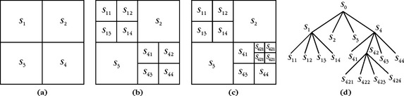
FIGURE 12.11 (a–c) Construction of a dyadic segmentation by successive subdivisions of squares. (d) Quad-tree representation of the segmentation. Each leaf of the tree corresponds to a square in the final segmentation.
The number of different geometric flows depends on the geometry’s required precision. Suppose that the edge curve in the square is parametrized horizontally and defined by (x1, γ(x1)). For a piecewise Cα image, γ(x1) is uniformly Lipschitz α. Tangent vectors to the edge are (1, γ′(x1)) and γ′(x1) is uniformly Lipschitz α – 1. If α ≤ q, then it can be approximated by a polynomial γ′ (x1) of degree q − 2 with
The polynomial γ′(x1) is specified by q − 1 parameters that must be quantized to limit the number of possible flows. To satisfy (12.42), these parameters are quantized with a precision 2−i. The total number of possible flows in the square of width 2i is thus O(2i(q−1)). A bandlet dictionary ![]() of order q is constructed with Cq wavelets having q vanishing moments, and with polynomial flows of degree q − 2.
of order q is constructed with Cq wavelets having q vanishing moments, and with polynomial flows of degree q − 2.
Bandlet Approximation
A best M-term bandlet signal approximation is computed by finding a best basis BT and the corresponding best approximation support ΛT, which minimize the 10 Lagrangian
This minimization chooses a best dyadic square segmentation of each wavelet coefficient array, and a best geometric flow in each square. It is implemented with the best-basis algorithm from Section 12.2.2.
An image ![]() is first approximated by its orthogonal projection in an approximation space VL of dimension N = 2−2L. The resulting discrete signal
is first approximated by its orthogonal projection in an approximation space VL of dimension N = 2−2L. The resulting discrete signal ![]() has the same wavelet coefficients as
has the same wavelet coefficients as ![]() at scales 2j > 2L, and thus the same bandlet coefficients at these scales. A best approximation support ΛT calculated from f yields an M = |ΛT| term approximation of
at scales 2j > 2L, and thus the same bandlet coefficients at these scales. A best approximation support ΛT calculated from f yields an M = |ΛT| term approximation of ![]() :
:
Theorem 12.5, proved in [342, 365], computes the nonlinear approximation error ![]() for piecewise regular images.
for piecewise regular images.
Theorem 12.5: Le Pennec, Mallat, Peyre. Let ![]() ∈ L2[0, 1]2 be a piecewise Cα regular image. In a bandlet dictionary of order q ≥ α, for T > 0 and 2L = N−1/2 ∼ T2,
∈ L2[0, 1]2 be a piecewise Cα regular image. In a bandlet dictionary of order q ≥ α, for T > 0 and 2L = N−1/2 ∼ T2,
For M = |ΛT|, the resulting best bandlet approximation ![]() M has an error
M has an error
Proof.
The proof finds a bandlet orthogonal basis ![]() such that
such that
Since ![]() , it implies (12.44). Theorem 12.1 derives in (12.5) that
, it implies (12.44). Theorem 12.1 derives in (12.5) that ![]() with
with ![]() . A piecewise regular image has a bounded total variation, so Theorem 9.18 proves that a linear approximation error with N larger-scale wavelets has an error
. A piecewise regular image has a bounded total variation, so Theorem 9.18 proves that a linear approximation error with N larger-scale wavelets has an error ![]() . Since
. Since ![]() , it results that
, it results that
which proves (12.45).
We give the main ideas for constructing a bandlet basis B that satisfies (12.46). Detailed derivations can be found in [365]. Following Definition 9.1, a function ![]() is piecewise Cα with a blurring scale
is piecewise Cα with a blurring scale ![]() where
where ![]() is uniformly Lipschitz α on
is uniformly Lipschitz α on ![]() , where the edge curves er are uniformly Lipschitz α and do not intersect tangentially. Since hs is a regular kernel of size s, the wavelet coefficients of
, where the edge curves er are uniformly Lipschitz α and do not intersect tangentially. Since hs is a regular kernel of size s, the wavelet coefficients of ![]() at a scale 2j behave as the wavelet coefficients of
at a scale 2j behave as the wavelet coefficients of ![]() at a scale 2j′ ∼ 2j + s multiplied by s−1. Thus, it has a marginal impact on the proof. We suppose that s = 0 and consider a signal
at a scale 2j′ ∼ 2j + s multiplied by s−1. Thus, it has a marginal impact on the proof. We suppose that s = 0 and consider a signal ![]() that is not blurred.
that is not blurred.
Wavelet coefficients ![]() are computed at scales 2j > 2L = T2. A dyadic segmentation of each wavelet coefficient array
are computed at scales 2j > 2L = T2. A dyadic segmentation of each wavelet coefficient array ![]() is computed according to Figure 12.8, at each scale 2j > 2L and orientation k = 1, 2, 3. Wavelet arrays are divided into three types of squares. In each type of square a geometric flow is specified, so that the resulting bandlet basis B has a Lagrangian that satisfies
is computed according to Figure 12.8, at each scale 2j > 2L and orientation k = 1, 2, 3. Wavelet arrays are divided into three types of squares. In each type of square a geometric flow is specified, so that the resulting bandlet basis B has a Lagrangian that satisfies ![]() . This is proved by verifying that the number of coefficients above T is O(T−2/(α + 1)) and that the energy of coefficients below T is O(T2−2/(α + 1)).
. This is proved by verifying that the number of coefficients above T is O(T−2/(α + 1)) and that the energy of coefficients below T is O(T2−2/(α + 1)).
![]() Regular squares correspond to coefficients
Regular squares correspond to coefficients ![]() , such that f is uniformly Lipschitz α over the support of all
, such that f is uniformly Lipschitz α over the support of all ![]() .
.
![]() Edge squares include coefficients corresponding to wavelets with support that intersects a single edge curve. This edge curve can be parametrized horizontally or vertically in each square.
Edge squares include coefficients corresponding to wavelets with support that intersects a single edge curve. This edge curve can be parametrized horizontally or vertically in each square.
![]() Junction squares include coefficients corresponding to wavelets with support that intersects at least two different edge curves.
Junction squares include coefficients corresponding to wavelets with support that intersects at least two different edge curves.
Over regular squares, since ![]() is uniformly Lipschitz α, Theorem 915 proves in (9.15) that
is uniformly Lipschitz α, Theorem 915 proves in (9.15) that ![]() . These small wavelet coefficients do not need to be retransformed and no geometric flow is defined over these squares. The number of coefficients above T in such squares is indeed O(T−2/(α + 1)) and the energy of coefficients below T is O(T2−2/(α + 1)).
. These small wavelet coefficients do not need to be retransformed and no geometric flow is defined over these squares. The number of coefficients above T in such squares is indeed O(T−2/(α + 1)) and the energy of coefficients below T is O(T2−2/(α + 1)).
Since edges do not intersect tangentially, one can construct junction squares of width 2i ≤ C where C does not depend on 2j. As a result, over the |log2 T2| scales 2j ≥ T2, there are only O(|log2T|) wavelet coefficients in these junction squares, which thus have a marginal impact on the approximation.
At a scale 2j, an edge square S of width 2i has O(2i2−j) large coefficients having an amplitude O(2j) along the edge. Bandlets are created to reduce the number of these large coefficients that dominate the approximation error. Suppose that the edge curve in S is parametrized horizontally and defined by (x1, y(x1)). Following (12.42), a geometric flow of vectors (1, γ′(x1)) is defined over the square, where γ′(x1) is a polynomial of degree q − 2, which satisfies
Let ![]() be the warping that maps this flow to a horizontal flow, as illustrated in Figure 12.9. One can prove [365] that the warped wavelet transform satisfies
be the warping that maps this flow to a horizontal flow, as illustrated in Figure 12.9. One can prove [365] that the warped wavelet transform satisfies
The bandlet transform takes advantage of the regularity of ![]() along x1 with Alpert directional wavelets having q vanishing moments along x1. Computing the amplitude of the resulting bandlet coefficients shows that there are
along x1 with Alpert directional wavelets having q vanishing moments along x1. Computing the amplitude of the resulting bandlet coefficients shows that there are ![]() bandlet coefficients of amplitude larger than T and the error of all coefficients below T is
bandlet coefficients of amplitude larger than T and the error of all coefficients below T is ![]() . The total length of edge squares is proportional to the total length of edges in the image, which is O(1). Summing the errors over all squares gives a total number of bandlet coefficients, which is
. The total length of edge squares is proportional to the total length of edges in the image, which is O(1). Summing the errors over all squares gives a total number of bandlet coefficients, which is ![]() , and a total error, which is
, and a total error, which is ![]() .
.
As a result, the bandlet basis B defined over the three types of squares satisfies ![]() , which finishes the proof.
, which finishes the proof.
The best-basis algorithm finds a best geometry to approximate each image. This theorem proves that the resulting approximation error decays as quickly as if the image was uniformly Lipschitz α over its whole support [0, 1]2. Moreover, this result is adaptive in the sense that it is valid for all α ≤ q.
The downside of bandlet approximations is the dictionary size. In a square of width 2i, we need ![]() polynomial flows, each of which defines a new bandlet family. As a result, a bandlet dictionary of order q includes
polynomial flows, each of which defines a new bandlet family. As a result, a bandlet dictionary of order q includes ![]() different bandlets. The total number of operations to compute a best bandlet approximation is O(P), which becomes very large for q > 2. A fast implementation is described in [398] for q = 2 where P = (N3/2). Theorem 12.5 is then reduced to α ≤ 2. It still recovers the O(M−2) decay for C2 images obtained in Theorem 9.19 with piecewise linear approximations over an adaptive triangulation.
different bandlets. The total number of operations to compute a best bandlet approximation is O(P), which becomes very large for q > 2. A fast implementation is described in [398] for q = 2 where P = (N3/2). Theorem 12.5 is then reduced to α ≤ 2. It still recovers the O(M−2) decay for C2 images obtained in Theorem 9.19 with piecewise linear approximations over an adaptive triangulation.
Figure 12.12 shows a comparison of the approximation of a piecewise regular image with M largest orthogonal wavelet coefficients and the best M orthogonal bandlet coefficients. Wavelet approximations exhibit more ringing artifacts along edges because they do not capture the anisotropic regularity of edges.
Bandlet Compression
Following the results of Section 12.1.2, a bandlet compression algorithm is implemented by quantizing the best bandlet coefficients of f with a bin size Δ = 2T. According to Section 12.1.2, the approximation support ΛT is coded on Ro = M log2(P/N) bits and the amplitude of nonzero quantized coefficients with R1 ˜ M bits [365]. If f is the discretization of apiecewise Cα image ![]() , since Lo(T,f,ΛT)=O(T2–2/(α+1)), we derive from (12.17) with s = (α+1)/2 that the distortion rate satisfies
, since Lo(T,f,ΛT)=O(T2–2/(α+1)), we derive from (12.17) with s = (α+1)/2 that the distortion rate satisfies
Analog piecewise Cα images are linearly approximated in a multiresolution space of dimension N with an error ![]() . Taking this into account, we verify that the analog distortion rate satisfies the asymptotic decay rate (12.18)
. Taking this into account, we verify that the analog distortion rate satisfies the asymptotic decay rate (12.18)
Although bandlet compression improves the asymptotic decay of wavelet compression, such coders are not competitive with a JPEG-2000 wavelet image coder, which requires less computations. Moreover, when images have no geometric regularity, despite the fact that the decay rate is the same as with wavelets, bandlets introduce an overhead because of the large dictionary size.
Bandlet Denoising
Let W be a Gaussian white noise of variance σ2. To estimate f from X = f + W, abest bandlet estimator ![]() is computed according to Section 12.2.1 by projecting X on an optimized family of orthogonal bandlets indexed by
is computed according to Section 12.2.1 by projecting X on an optimized family of orthogonal bandlets indexed by ![]() . It is obtained by thresholding at T the bandlet coefficients of X in the best bandlet basis
. It is obtained by thresholding at T the bandlet coefficients of X in the best bandlet basis ![]() , which minimizes Lo(T,X,B),for
, which minimizes Lo(T,X,B),for![]() .
.
An analog estimator ![]() of
of ![]() is reconstructed from the noisy signal coefficients in
is reconstructed from the noisy signal coefficients in ![]() with the analog bandlets
with the analog bandlets ![]() . If
. If ![]() is a piecewise Cα image
is a piecewise Cα image ![]() , then Theorem 12.5 proves that
, then Theorem 12.5 proves that ![]() . The computed risk decay (12.27) thus applies for s = (α+ 1)/2:
. The computed risk decay (12.27) thus applies for s = (α+ 1)/2:
This decay rate [233] shows that a bandlet estimation over piecewise Cα images nearly reaches the minimax risk ![]() calculated in (11.152) for uniformly Cα images. Figure 12.13 gives a numerical example comparing a best bandlet estimation and a translation-invariant wavelet thresholding estimator for an image including regular geometric structures. The threshold is T = 3σ instead of
calculated in (11.152) for uniformly Cα images. Figure 12.13 gives a numerical example comparing a best bandlet estimation and a translation-invariant wavelet thresholding estimator for an image including regular geometric structures. The threshold is T = 3σ instead of ![]() , because it improves the SNR.
, because it improves the SNR.
12.3 GREEDY MATCHING PURSUITS
Computing an optimal M-term approximation fM of a signal f with M vectors selected in a redundant dictionary ![]() is NP-hard. Pursuit strategies construct nonoptimal yet efficient approximations with computational algorithms. Matching pursuits are greedy algorithms that select the dictionary vectors one by one, with applications to compression, denoising, and pattern recognition.
is NP-hard. Pursuit strategies construct nonoptimal yet efficient approximations with computational algorithms. Matching pursuits are greedy algorithms that select the dictionary vectors one by one, with applications to compression, denoising, and pattern recognition.
12.3.1 Matching Pursuit
Matching pursuit introduced by Mallat and Zhang [366] computes signal approximations from a redundant dictionary, by iteratively selecting one vector at a time. It is related to projection pursuit algorithms used in statistics [263] and to shape-gain vector quantizations [27].
Let ![]() be a dictionary of P > N vectors having a unit norm. This dictionary is supposed to be complete, which means that it includes N linearly independent vectors that define a basis of the signal space
be a dictionary of P > N vectors having a unit norm. This dictionary is supposed to be complete, which means that it includes N linearly independent vectors that define a basis of the signal space ![]() . A matching pursuit begins by projecting f on a vector
. A matching pursuit begins by projecting f on a vector ![]() and by computing the residue Rf:
and by computing the residue Rf:
To minimize ![]() , we must choose
, we must choose ![]() such that
such that ![]() is maximum. In some cases it is computationally more efficient to find a vector φpo that is almost optimal:
is maximum. In some cases it is computationally more efficient to find a vector φpo that is almost optimal:
where α ∈ (0, 1] is a relaxation factor. The pursuit iterates this procedure by sub-decomposing the residue. Let R0f = f. Suppose that the mth-order residue Rmf is already computed for m ≥ 0. The next iteration chooses ![]() such that
such that
and projects Rmf on ![]() :
:
The orthogonality of Rm+1f and ![]() implies
implies
Summing (12.52) from m between 0 and M – 1 yields
 (12.54)
Similarly, summing (12.53) from m between 0 and M – 1 gives
 (12.55)
Convergence of Matching Pursuit
A matching pursuit has an exponential decay if the residual ![]() has a minimum rate of decay. The conservation of energy (12.53) implies
has a minimum rate of decay. The conservation of energy (12.53) implies
where ![]() is the coherence of a vector relative to the dictionary, defined by
is the coherence of a vector relative to the dictionary, defined by
Theorem 12.6 proves that
and thus that matching pursuits converge exponentially.
Theorem 12.6.
The residual Rmf computed by a matching pursuit with relaxation parameter α ∈ (0, 1] satisfies
 (12.58)
Proof.
The atom ![]() selected by a matching pursuit satisfies
selected by a matching pursuit satisfies ![]() . It results from (12.56) that
. It results from (12.56) that
Iterating on this equation proves that
To verify that ![]() , a contrario lets us suppose that
, a contrario lets us suppose that ![]() . There exist
. There exist ![]() with
with ![]() such that
such that
Since the unit sphere of ![]() is compact, there exists a subsequence
is compact, there exists a subsequence ![]() that converges to a unit vector
that converges to a unit vector ![]() . It follows that
. It follows that
so ![]() for all
for all ![]() . Since
. Since ![]() contains a basis of
contains a basis of ![]() , necessarily f = 0, which is not possible because
, necessarily f = 0, which is not possible because ![]() . It results that, necessarily,
. It results that, necessarily, ![]() .
.
This proves that ![]() and thus that
and thus that ![]() . Inserting this in (12.54) and (12.55) proves (12.58).
. Inserting this in (12.54) and (12.55) proves (12.58).
Matching pursuits often converge more slowly when the size N of the signal space increases because ![]() can become close to 0. In the limit of infinite-dimensional spaces, Jones’ theorem proves that the matching pursuit still converges but the convergence is not exponential [319, 366]. Section 12.3.2 describes an orthogonalized matching pursuit that converges in fewer than N iterations.
can become close to 0. In the limit of infinite-dimensional spaces, Jones’ theorem proves that the matching pursuit still converges but the convergence is not exponential [319, 366]. Section 12.3.2 describes an orthogonalized matching pursuit that converges in fewer than N iterations.
Backprojection
matching pursuit computes an approximation ![]() that belongs to space VM generated by M vectors
that belongs to space VM generated by M vectors ![]() . However, in general
. However, in general ![]() is not equal to the orthogonal projection fM on f in VM, and thus
is not equal to the orthogonal projection fM on f in VM, and thus ![]() . In finite dimension, an infinite number of matching pursuit iterations is typically necessary to completely remove the error
. In finite dimension, an infinite number of matching pursuit iterations is typically necessary to completely remove the error ![]() , although in most applications this approximation error becomes sufficiently small for M
, although in most applications this approximation error becomes sufficiently small for M ![]() N. To reduce the matching pursuit error, Mallat and Zhang [366] introduced a backprojection that computes the coefficients
N. To reduce the matching pursuit error, Mallat and Zhang [366] introduced a backprojection that computes the coefficients ![]() of the orthogonal projection
of the orthogonal projection

Let ![]() . Section 5.1.3 shows that the decomposition coefficients of this dual-analysis problem are obtained by inverting the Gram operator
. Section 5.1.3 shows that the decomposition coefficients of this dual-analysis problem are obtained by inverting the Gram operator

This inversion can be computed with a conjugate-gradient algorithm or with a Richardson gradient descent from the initial coefficients ![]() provided by the matching pursuit. Let γ be a relaxation parameter that satisfies
provided by the matching pursuit. Let γ be a relaxation parameter that satisfies
where BM≥AM>0 are the frame bounds of ![]() in VM. Theorem 5.7 proves that
in VM. Theorem 5.7 proves that
converges to the solution: ![]() . A safe choice is γ = 2/B where B ≥ BM is the upper frame bound of the overall dictionary
. A safe choice is γ = 2/B where B ≥ BM is the upper frame bound of the overall dictionary ![]() .
.
Fast Network Calculations
A matching pursuit is implemented with a fast algorithm that computes ![]() from
from ![]() with an updating formula. Taking an inner product with φp on each side of (12.52) yields
with an updating formula. Taking an inner product with φp on each side of (12.52) yields
In neural network language, this is an inhibition of ![]() by the selected pattern φpm with a weight
by the selected pattern φpm with a weight ![]() that measures its correlation with φp. To reduce the computational load, it is necessary to construct dictionaries with vectors having a sparse interaction. This means that each
that measures its correlation with φp. To reduce the computational load, it is necessary to construct dictionaries with vectors having a sparse interaction. This means that each ![]() has nonzero inner products with only a small fraction of all other dictionary vectors. It can also be viewed as a network that is not fully connected. Dictionaries can be designed so that nonzero weights
has nonzero inner products with only a small fraction of all other dictionary vectors. It can also be viewed as a network that is not fully connected. Dictionaries can be designed so that nonzero weights ![]() are retrieved from memory or computed with O(1) operations. A matching pursuit with a relative precision ε is implemented with the following steps:
are retrieved from memory or computed with O(1) operations. A matching pursuit with a relative precision ε is implemented with the following steps:
then stop. Otherwise, m = m + 1 and go to 2.
If ![]() is very redundant, computations at steps 1, 2, and 3 are reduced by performing the calculations in a subdictionary
is very redundant, computations at steps 1, 2, and 3 are reduced by performing the calculations in a subdictionary ![]() . The subdictionary
. The subdictionary ![]() is constructed so that if
is constructed so that if ![]() , then
, then
The selected atom ![]() is improved with a local search in the larger dictionary
is improved with a local search in the larger dictionary ![]() , among all atoms φp “close” to
, among all atoms φp “close” to ![]() , in the sense that
, in the sense that ![]() for a predefined constant C. This local search finds φpm, which locally maximizes the residue correlation
for a predefined constant C. This local search finds φpm, which locally maximizes the residue correlation
The updating (12.64) is restricted to vectors ![]() . The construction of hierarchical dictionaries can also reduce the calculations needed to compute inner products in
. The construction of hierarchical dictionaries can also reduce the calculations needed to compute inner products in ![]() from inner products in
from inner products in ![]() [387].
[387].
The dictionary must incorporate important signal features, which depend on the signal class. Section 12.3.3 studies dictionaries of Gabor atoms. Section 12.3.4 describes applications to noise reduction. Specific dictionaries for inverse electromagnetic problems, face recognition, and data compression are constructed in [80, 374, 399]. Dictionary learning is studied in Section 12.7.
Wavelet Packets and Local Cosines Dictionaries
Wavelet packet and local cosine trees constructed in Sections 8.2.1 and 8.5.3 are dictionaries with P = N log2 N vectors. For each dictionary vector, there are few other dictionary vectors having nonzero inner products that can be stored in tables to compute the updating formula (12.64). Each matching pursuit iteration then requires O(N log2 N) operations.
In a dictionary of wavelet packet bases calculated with a Daubechies 8 filter, the best basis shown in Figure 12.14(c) optimizes the division of the frequency axis, but it has no flexibility in time. It is, therefore, not adapted to the time evolution of the signal components. The matching pursuit flexibility adapts the wavelet packet choice to local signal structures; Figure 12.14(d) shows that it better reveals its time-frequency properties than the best wavelet packet basis.
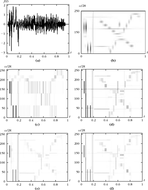
FIGURE 12.14 (a) Signal synthesized with a sum of chirps, truncated sinusoids, short time transients, and Diracs. The time-frequency images display the atoms selected by different adaptive time-frequency transforms. The darkness is proportional to the coefficient amplitude. (b) Gabor matching pursuit. Each dark blob is the Wigner-Ville distribution of a selected Gabor atom. (c) Heisenberg boxes of a best wavelet packet basis calculated with a Daubechies 8 filter. (d) Wavelet packets selected by a matching pursuit. (e) Wavelet packets of a basis pursuit. (f) Wavelet packets of an orthogonal matching pursuit.
Translation Invariance
Representing a signal structure independently from its location is a form of translation invariance that is important for pattern recognition. Decompositions in orthonormal bases lack this translation invariance. Matching pursuits are translation invariant if calculated in translation-invariant dictionaries. A dictionary ![]() is translation invariant if for any
is translation invariant if for any ![]() , then
, then ![]() for 0 ≤ p N. Suppose that the matching decomposition of f in
for 0 ≤ p N. Suppose that the matching decomposition of f in ![]() is [201]
is [201]
 (12.66)
Then the matching pursuit of fp[n] = f[n – p] selects a translation by p of the same vectors φpm with the same decomposition coefficients

Thus, patterns can be characterized independently of their position.
Translation invariance is generalized as an invariance with respect to any group action [201]. A frequency translation is another example of a group operation. If the dictionary is invariant under the action of a group, then the pursuit remains invariant under the action of the same group. Section 12.3.3 gives an example of a Gabor dictionary, which is translation invariant in time and frequency.
12.3.2 Orthogonal Matching Pursuit
Matching pursuit approximations are improved by orthogonalizing the directions of projection with a Gram-Schmidt procedure. The resulting orthogonal pursuit converges with a finite number of iterations. This orthogonalization was introduced by Mallat and Zhang together with the nonorthogonal pursuit algorithm in Zhang thesis [74]. The higher computational cost of the Gram-Schmidt algorithm may seem discouraging (reviewers suppressed it from the first publication in [366]), but the improved precision of this orthogonalization becomes important for the inverse problems studied in Chapter 13. It appeared in [202] and was proposed independently by Pati, Rezaifar, and Krishnaprasad [395].
The vector φpm selected by the matching algorithm is a priori not orthogonal to the previously selected vectors {φpl}0≤l<m. When subtracting the projection of Rmf over φpm, the algorithm reintroduces new components in the directions of {φpl}0≤l<m. This is avoided by projecting the residues on an orthogonal family {ul}0≤l<m computed from {φpl}0≤l<m.
Let us initialize u0 = φp0. For m ≥ 0, an orthogonal matching pursuit selects φpm that satisfies
The Gram-Schmidt algorithm orthogonalizes φpm with respect to {φpl}0≤l<m and defines
 (12.68)
The residue Rmf is projected on um instead of φpm:
Summing this equation for 0 ≤ m < k yields
 (12.70)
where Pvk is the orthogonal projector on the space Vk generated by {um}0≤m<k. The Gram-Schmidt algorithm ensures that {φpm}0≤m<k is also a basis of Vk. For any k ≥ 0 the residue Rkf is the component of f that is orthogonal to Vk. For m = k, (12.68) implies that
Since Vk has dimension k there exists M ≤ N, but most often M = N, such that f ∈ VM, so RMf = 0 and inserting (12.71) in (12.70)for k = M yields
 (12.72)
The algorithm stops after M ≤ N iterations. The energy conservation resulting from this decomposition in a family of orthogonal vectors is
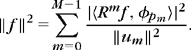 (12.73)
The exponential convergence rate of the matching pursuit in Theorem 12.6 remains valid for an orthogonal matching pursuit, but it also converges in less than N iterations.
To expand f over the original dictionary vectors {φpm}0≤m<M, we must perform a change of basis. The triangular Gram-Schmidt relations (12.68) are inverted to expand um in {φpk}0≤k<m:
Inserting this expression into (12.72) gives
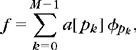 (12.75)
with

The Gram-Schmidt summation (12.68) must be carefully implemented to avoid numerical instabilities [29]. A Gram-Schmidt orthogonalization of M vectors requires O(NM2) operations. In wavelet packet, local cosine, and Gabor dictionaries, M matching pursuit iterations are calculated with O(MN log2 N) operations.
For M large, the Gram-Schmidt orthogonalization very significantly increases the computational complexity of a matching pursuit. A final matching pursuit orthogonal backprojection requires at most O(M3) operators, but both algorithms may not give the same results because they do not necessarily select the same vectors. An orthogonal pursuit can improve the approximation precision as shown in Sections 13.3 and 13.4 for the resolution of inverse problems.
Figure 12.14(f) displays the wavelet packets selected by an orthogonal matching pursuit. A comparison with Figure 12.14(d) shows that the orthogonal and nonorthogonal pursuits select nearly the same wavelet packets having a high-amplitude inner product. These vectors are called coherent structures. They are selected during the first few iterations. A mathematical interpretation of these coherent structures is given in Section 12.5.2. Most often, during the first few iterations, a matching pursuit selects nearly orthogonal vectors, so orthogonal and nonorthogonal pursuits are nearly identical. When the number of iterations increases and gets close to N, the residues of an orthogonal pursuit have norms that decrease faster than for a nonorthogonal pursuit. For large-size signals, where the number of iterations is a small fraction of N, the nonorthogonal pursuit is more often used, but the orthogonalization or a backprojection becomes important if a high-approximation precision is needed.
12.3.3 Gabor Dictionaries
Gabor dictionaries are constructed with Gaussian windows, providing optimal time and frequency energy concentration. For images, directional Gabor dictionaries lead to efficient representations, particularly for video compression.
Time-Frequency Gabor Dictionary
A time and frequency translation-invariant Gabor dictionary is constructed by Qian and Chen [405] as well as Mallat and Zhang [366], by scaling, modulating, and translating a Gaussian window on the signal-sampling grid. For each scale 2j, a discrete Gaussian window is defined by
where the constant Kj ≈ 1 is adjusted so that ![]() . A Gabor time-frequency frame is derived with time intervals uj = 2jΔ−1 and frequency intervals ξj = 2πΔ−12−j:
. A Gabor time-frequency frame is derived with time intervals uj = 2jΔ−1 and frequency intervals ξj = 2πΔ−12−j:
It includes P = Δ2N vectors. Asymptotically for N large, this family of Gabor signals has the same properties as the frames of the Gabor functions studied in Section 5.4.
Theorem 5.19 proves that a necessary condition to obtain a frame is that uj ξj = 2πΔ−2 < 2π, and thus Δ > 1. Table 5.3 shows that for Δ ≥ 2, this Gabor dictionary is nearly a tight frame with A ≈ B ≈ Δ2.
A multiscale Gabor dictionary is a union of such tight frames
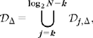 (12.78)
 with typically k ≤ 2 to avoid having too-small or too-large windows. Its size is thus P ≤ Δ2N log2 N, and for Δ ≥, 2 it is nearly a tight frame with frame bounds Δ2 log2 N. A translation-invariant dictionary is a much larger dictionary obtained by setting uj = 1 and ξj = 2π/N in (12.77), and it thus includes P ≈ N2 log2 N vectors.
A matching pursuit decomposes real signals in the multiscale Gabor dictionary (12.78) by grouping atoms φp+ and φp− with p± = (quj, ± kξj, 2j). At each iteration, instead of projecting Rmf over an atom φp, the matching pursuit computes its projection on the plane generated by (φp+, φp−). Since Rmf[n] is real, one can verify that this is equivalent to projecting Rmf on a real vector that can be written as
The constant Kj,γ sets the norm of this vector to 1 and the phase γ is optimized to maximize the inner product with Rmf. Matching pursuit iterations yield
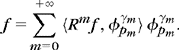 (12.79)
The time-frequency signal geometry is characterized by the time-frequency and scale support ![]() of the M selected Gabor atoms. It is more easily visualized with a time-frequency energy distribution obtained by summing the Wigner-Ville distribution Pvφpm[n, k] of the complex atoms φpm:
of the M selected Gabor atoms. It is more easily visualized with a time-frequency energy distribution obtained by summing the Wigner-Ville distribution Pvφpm[n, k] of the complex atoms φpm:
 (12.80)
Since the window is Gaussian, Pvφpm is a two-dimensional Gaussian blob centered at (qmujm, kmξjm) in the time-frequency plane. It is scaled by 2jm in time and by N2−jm in frequency.
Computations
A matching pursuit in a translation-invariant Gabor dictionary of size P = N2log2 N is implemented by restricting most computations in the multiscale dictionary ![]() of smaller size P ≤ 4Nlog2N for Δ = 2. At each iteration, a Gabor atom
of smaller size P ≤ 4Nlog2N for Δ = 2. At each iteration, a Gabor atom ![]() that best matches Rmf is selected in
that best matches Rmf is selected in ![]() . The position and frequency of this atom are then refined with (12.65). It finds a close time-frequency atom φpm in the larger translation-invariant dictionary, which has a better correlation with Rmf. The inner product update (12.64) is then computed only for atoms in
. The position and frequency of this atom are then refined with (12.65). It finds a close time-frequency atom φpm in the larger translation-invariant dictionary, which has a better correlation with Rmf. The inner product update (12.64) is then computed only for atoms in ![]() , with an analytical formula. Two Gabor atoms that have positions, frequencies, and scales p1 = (u1, ξ1, s1) and p2 = (u2, ξ2, s2) have an inner product
, with an analytical formula. Two Gabor atoms that have positions, frequencies, and scales p1 = (u1, ξ1, s1) and p2 = (u2, ξ2, s2) have an inner product
 (12.81)
The error terms can be neglected if the scales s1 and s2 are not too small or too close to N. The resulting matching pursuit in a translation-invariant Gabor dictionary requires marginally more computations than a matching pursuit in ![]() .
.
Figure 12.14(b) shows the matching pursuit decomposition of a signal having localized time-frequency structures. This representation is more sparse than the matching pursuit decomposition in the wavelet packet dictionary shown in Figure 12.14(d). Indeed, Gabor dictionary atoms are translated on a finer time-frequency grid than wavelet packets, and they have a better time-frequency localization. As a result, the matching pursuits find Gabor atoms that better match the signal structures.
Figure 12.15 gives the Gabor matching pursuit decomposition of the word “greasy,” sampled at 16 kHz. The time-frequency energy distribution shows the low-frequency component of the “g” and the quick-burst transition to the “ea.” The “ea” has many harmonics that are lined up. The “s” is a noise with a time-frequency energy spread over a high-frequency interval. Most of the signal energy is characterized by a few time-frequency atoms. For m = 250 atoms, ![]() , even though the signal has 5782 samples, and the sound recovered from these atoms is of good audio quality.
, even though the signal has 5782 samples, and the sound recovered from these atoms is of good audio quality.

FIGURE 12.15 Speech recording of the word “greasy” sampled at 16 kHz. In the time-frequency image, the dark blobs of various sizes are the Wigner-Ville distributions of Gabor functions selected by the matching pursuit.
Matching pursuits in Gabor dictionaries provide sparse representation of oscillatory signals, with frequency and scale parameters that are used to characterize the signal structures. For example, studies have been carried in cognitive neurophysiology for the analysis of gamma and high-gamma oscillations in electroencephalogram (EEG) signals [406], which are highly nonstationary. Matching pursuit decompositions are also used to predict epilepsy patterns [22], allowing physicians to identify periods of seizure initiation by analyzing the selected atom properties [259, 320].
In Figure 12.14(b), the two chirps with frequencies that increase and decrease linearly are decomposed in many Gabor atoms. To improve the representation of signals having time-varying spectral lines, the dictionary can include Gabor chirps having an instantaneous frequency that varies linearly in time:
Their Wigner-Ville distribution PvφP[n, k] is localized around an oriented segment in the time-frequency plane. Such atoms can more efficiently represent progressive frequency variations of the signal spectral components. However, increasing the dictionary size also increases intermediate memory storage and computational complexity. To incorporate Gabor chirps, Gribonval [278] reduces the matching pursuit complexity by first optimizing the scale-time-frequency parameters (2j, q, k) for c = 0, and then adjusting c instead of jointly optimizing all parameters.
Directional Image Gabor Dictionaries
A sparse representation of image structures such as edges, corners, and textures requires using a large dictionary of vectors. Section 5.5.1 describes redundant dictionaries of directional wavelets and curvelets. Matching pursuit decompositions over two-dimensional directional Gabor wavelets are introduced in [105]. They are constructed with a separable product of Gaussian windows gj[n] in (12.76), with angle directions ![]() where
where ![]() is typically 4 or 8:
is typically 4 or 8:
with Δ ≥ 2 and ε < 2π. This dictionary is a redundant directional wavelet frame. As opposed to the frame decompositions in Section 5.5.1, a matching pursuit yields a sparse image representation by selecting a few Gabor atoms best adapted to the image.
Figure 12.16 shows the atoms selected by a matching pursuit on the Lena image. Each selected atom is displayed as an ellipse at a position 2jΔ−1 (q1, q2), of width proportional to 2j and oriented in direction θ, with a grayscale amplitude proportional to the matching pursuit coefficient.
FIGURE 12.16 Directional Gabor wavelets selected by a matching pursuit at several scales 2j: (a) 21, (b) 22, and (c) 23. Each ellipse gives the direction, scale, and position of a selected Gabor atom.
To better capture the anisotropic regularity of edges, more Gabor atoms are incorporated in the dictionary, with an anisotropic stretching of their support. This redundant dictionary, which includes directional wavelets and curvelets, can be applied to low-bit rate image compression [257].
Video Compression
In MPEG-1, -2, -4 video compression standards, motion vectors are coded to predict an image from a previous one, with a motion compensation [156, 437]. Figure 12.17(b) shows a prediction error image. It is the difference between the image in Figure 12.17(a) and a prediction obtained by moving pixel blocks of a previous image by using computed motion vectors. When the motion is not accurate, it yields errors along edges and sharp structures. These errors typically define oriented oscillatory structures. In MPEG compression standards, prediction error images are compressed with the discrete cosine transform (DCT) introduced in Section 8.3.3. The most recent MPEG-4 H.264 standard adapts the size and shape of the DCT blocks to optimize the distortion rate.

FIGURE 12.17 (a) Image of video sequences with three cars moving on a street. (b) Motion compensation error.
Neff and Zakhor [386] introduced a video matching pursuit compression in two-dimensional Gabor dictionaries that efficiently compresses prediction error images. Section 12.1.2 explains that an orthogonalization reduces the quantization error, but the computational complexity of the orthogonalization is too important for real-time video calculations. Compression is thus implemented with a nonorthogonal matching pursuit iteration (12.52), modified to quantize the selected inner product with Q(x):
Initially implemented in a separable Gabor dictionary [386], this procedure is refined in hierarchical dictionaries providing fast algorithms for larger directional Gabor dictionaries, which improves the compression efficiency [387]. Other dictionaries reducing computations have been proposed [80, 191, 318, 351, 426], with distortion rate models to adjust the quantizer to the required bit budget [388]. This lead to a video coder, recognized in 2002 by the MPEG-4 standard expert group as having the best distortion rate with a realistic implementation among all existing solutions. However, industrial priorities have maintained a DCT solution for the new MPEG-4 standard.
12.3.4 Coherent Matching Pursuit Denoising
If we cannot interpret the information carried by a signal component, it is often misconstrued as noise. In a crowd speaking a foreign language, we perceive surrounding conversations as background noise. In contrast, our attention is easily attracted by a remote conversation spoken in a known language. What is important here is not the information content but whether this information is in a coherent format with respect to our system of interpretation. The decomposition of a signal in a dictionary of vectors can similarly be considered as a signal interpretation. Noises are then defined as signal components that do not have a strong correlation with any vector of the dictionary. In the absence of any knowledge concerning the noise, Mallat and Zhang [366] introduced a coherent matching pursuit denoising that selects coherent structures having a high correlation with vectors in the dictionary. These coherent structures typically correspond to the approximation support of f that can be identified in ![]() .
.
Denoising by Thresholding
Let X[n] = f[n] + W[n] be noisy measurements. The dictionary estimator of Theorem 12.3 in Section 12.1.3 projects X on a best set of dictionary vectors Λ ⊂ Γ, which minimizes the 10 Lagrangian ![]() .
.
For an orthogonal matching pursuit approximation that selects one by one the vectors that are orthogonalized, this is equivalent to thresholding at T the resulting decomposition (12.72):

Since the amplitude of residual coefficients ![]() almost systematically decreases as m increases, it is nearly equivalent to stop the matching pursuit decomposition at the first iteration M such that
almost systematically decreases as m increases, it is nearly equivalent to stop the matching pursuit decomposition at the first iteration M such that ![]() Thus, the threshold becomes a stopping criteria.
Thus, the threshold becomes a stopping criteria.
For a nonorthogonal matching pursuit, despite the nonorthogonality of selected coefficients, a denoising algorithm can also be implemented by stopping the decomposition (12.58) as soon as ![]() . The resulting estimator is
. The resulting estimator is

and can be optimized with a back projection computing the orthogonal projection of X in {φpm}0 ≤ m < M. Coherent denoising provides a different approach that does not rely on a particular noise model and does not set in advance the threshold T.
Coherent Denoising
A coherent matching pursuit denoising selects signal structures having a correlation with dictionary vectors that is above an average defined over a matching pursuit attractor. A matching pursuit behaves like a nonlinear chaotic map, and it has been proved by Davis, Mallat, and Avellaneda [201] that for particular dictionaries, the normalized residues ![]() converge to an attractor. This attractor is a set of normalized signals h that do not correlate well with any
converge to an attractor. This attractor is a set of normalized signals h that do not correlate well with any ![]() because all coherent structures of f producing maximum inner products with vectors in
because all coherent structures of f producing maximum inner products with vectors in ![]() are progressively removed by the pursuit. Signals on the attractor do not correlate well with any dictionary vector and are thus considered as an incoherent noise with respect to
are progressively removed by the pursuit. Signals on the attractor do not correlate well with any dictionary vector and are thus considered as an incoherent noise with respect to ![]() . The coherence of f relative to
. The coherence of f relative to ![]() is defined in (12.3.1) by
is defined in (12.3.1) by ![]() . For signals in the attractor, this coherence has a small amplitude, and we denote the average coherence of this attractor as
. For signals in the attractor, this coherence has a small amplitude, and we denote the average coherence of this attractor as ![]() , which depends on
, which depends on ![]() [201]. This average coherence is defined by
[201]. This average coherence is defined by
where W′ is a Gaussian white noise of variance σ2 = 1. The bottom regular curve C in Figure 12.18 gives the value of ![]() that is nearly equal to
that is nearly equal to ![]() for m ≥ 40 in a Gabor dictionary.
for m ≥ 40 in a Gabor dictionary.

FIGURE 12.18 Decay of the correlation ![]() as a function of the number of iterations m for two signals decomposed in a Gabor dictionary. A: f is the recording of “greasy” shown in Figure 12.19(a). B: f is the noisy “greasy” signal shown in Figure 12.19(b). C:
as a function of the number of iterations m for two signals decomposed in a Gabor dictionary. A: f is the recording of “greasy” shown in Figure 12.19(a). B: f is the noisy “greasy” signal shown in Figure 12.19(b). C: ![]() that is for a normalized Gaussian white noise W′.
that is for a normalized Gaussian white noise W′.
The convergence of the pursuit to the attractor implies that for m ≥ M iterations, the residue Rmf has a normalized correlation ![]() that is nearly equal to
that is nearly equal to ![]() . Curve A in Figure 12.18 gives the decay of
. Curve A in Figure 12.18 gives the decay of ![]() as a function of m for the “greasy” signal f in Figure 12.19(a). After about M = 1400 iterations, it reaches the average coherence level of the attractor. The corresponding 1400 time-frequency atoms are shown in Figure 12.15. Curve B in Figure 12.18 shows the decay of
as a function of m for the “greasy” signal f in Figure 12.19(a). After about M = 1400 iterations, it reaches the average coherence level of the attractor. The corresponding 1400 time-frequency atoms are shown in Figure 12.15. Curve B in Figure 12.18 shows the decay of ![]() for the noisy signal X = f + W in Figure 12.19(b), which has an SNR of 1.5 db. The high-amplitude noise destroys most coherent structures and the attractor is reached after M = 76 iterations.
for the noisy signal X = f + W in Figure 12.19(b), which has an SNR of 1.5 db. The high-amplitude noise destroys most coherent structures and the attractor is reached after M = 76 iterations.

FIGURE 12.19 (a) Speech recording of “greasy.” (b) Recording of “greasy” plus a Gaussian white noise (SNR = 1.5 db). (c) Time-frequency distribution of the M = 76 coherent Gabor structures. (d) Estimation ![]() reconstructed from the 76 coherent structures (SNR = 6.8 db).
reconstructed from the 76 coherent structures (SNR = 6.8 db).
A coherent matching pursuit denoising with a relaxation parameter α = 1 decomposes a signal as long as the coherence of the residue is above ![]() and stops after:
and stops after:

This estimator can thus also be interpreted as a thresholding of the matching pursuit of X with a threshold that is adaptively adjusted to
The time-frequency energy distribution of the M = 76 coherent Gabor atoms of the noisy signal is shown in Figure 12.19(c). The estimation ![]() calculated from the 76 coherent structures is shown in Figure 12.19(d). The SNR of this estimation is 6.8 db. The white noise has been removed with no estimation of the variance, and the restored speech signal has a good intelligibility because its main time-frequency components are retained.
calculated from the 76 coherent structures is shown in Figure 12.19(d). The SNR of this estimation is 6.8 db. The white noise has been removed with no estimation of the variance, and the restored speech signal has a good intelligibility because its main time-frequency components are retained.
12.4 I1 PURSUITS
To reduce inefficiencies produced by the greediness of matching pursuits, 11 pursuits perform a more global optimization, which replaces the 10 norm minimization of a best M-term approximation by an 11 norm. The 10 Lagrangian studied from Section 12.1.1 is thus replaced by the 11 Lagrangian from Section 12.4.2. Although they are not optimal in general, Section 12.5 proves that matching pursuits and basis pursuits can compute nearly optimal M-term approximations, depending on the signal approximation support and the dictionary.
12.4.1 Basis Pursuit
Each step of a matching pursuit performs a local optimization that can be fooled. A basis pursuit minimizes a global criterion that avoids some mistakes made by greedy pursuits. A simple but typical example of failure happens when a linear combination of two vectors f = φm + φq happens to be highly correlated with a third vector φr∈D. A matching pursuit may choose φr instead of φm or φq, and many other vectors are then needed to correct this wrong initial choice, which produces a nonoptimal representation.
Figure 12.20 illustrates this phenomenon with a dictionary ![]() of one-dimensional Gabor atoms specified in (12.77). Each Gabor function is a Gaussian translated in time and frequency with an oversampled time-frequency grid calculated with Δ = 1/4. It has P = 16N vectors of size N. Figure 12.20 shows a signal f = φm + φq where φm and φq are two Gabor functions having nearly the same position and frequency. Let σt and σω be the time and frequency variance of these Gabor atoms. Figure 12.20(b) represents these atoms in the time-frequency plane, with two reduced Heisenberg rectangles, of time width σt/Δ and frequency width σω/Δ, so that all dictionary coefficients can be visualized. The full-size Heisenberg boxes σt × σω of φm and φq overlap widely, which makes it difficult to discriminate them in f. Figures 12.20(c, d) show that a matching pursuit and an orthogonal matching pursuit select a first time-frequency atom with a time and frequency location intermediate between these two atoms, and then other subsequent vectors to compensate for this initial mistake. Such nonoptimal greedy choices are observed on real signals decomposed in redundant dictionaries. High-resolution greedy pursuits can reduce the loss of resolution in time with nonlinear correlation measures [279, 314], but the greediness can still have adverse effects.
of one-dimensional Gabor atoms specified in (12.77). Each Gabor function is a Gaussian translated in time and frequency with an oversampled time-frequency grid calculated with Δ = 1/4. It has P = 16N vectors of size N. Figure 12.20 shows a signal f = φm + φq where φm and φq are two Gabor functions having nearly the same position and frequency. Let σt and σω be the time and frequency variance of these Gabor atoms. Figure 12.20(b) represents these atoms in the time-frequency plane, with two reduced Heisenberg rectangles, of time width σt/Δ and frequency width σω/Δ, so that all dictionary coefficients can be visualized. The full-size Heisenberg boxes σt × σω of φm and φq overlap widely, which makes it difficult to discriminate them in f. Figures 12.20(c, d) show that a matching pursuit and an orthogonal matching pursuit select a first time-frequency atom with a time and frequency location intermediate between these two atoms, and then other subsequent vectors to compensate for this initial mistake. Such nonoptimal greedy choices are observed on real signals decomposed in redundant dictionaries. High-resolution greedy pursuits can reduce the loss of resolution in time with nonlinear correlation measures [279, 314], but the greediness can still have adverse effects.

FIGURE 12.20 (a) Signal f = φm + φq. (b) Reduced Heisenberg boxes of the two Gabor atoms Φm and Φq, shown in the time-frequency plane. (c) Atoms selected by a matching pursuit. The darkness of each box is proportional to selected coefficients’ amplitude. (d) Atoms selected by an orthogonal matching pursuit. (e) A basis pursuit recovers the two original atoms.
I1 Minimization
Avoiding this greediness suboptimality requires using a global criterion that enforces the sparsity of the decomposition coefficients of f in ![]() be the decomposition operator in
be the decomposition operator in ![]() The reconstruction from dictionary vectors is implemented by the adjoint (5.3)
The reconstruction from dictionary vectors is implemented by the adjoint (5.3)
 (12.82)
Since the dictionary is redundant, there are many possible reconstructions. The basis pursuit introduced by Chen and Donoho [159] finds the vector ![]() of coefficients having a minimum 11 norm
of coefficients having a minimum 11 norm
This is a convex minimization that can be written as a linear programming and is thus calculated with efficient algorithms, although computationally more intensive than a matching pursuit. If the solution of (12.83) is not unique, then any valid solution may be used.
The signal in Figure 12.20 can be written exactly as a sum of two dictionary vectors and the basis pursuit minimization recovers this best representation by selecting the appropriate dictionary vectors, as opposed to matching pursuit algorithms. Minimizing the 11 norm of the decomposition coefficients a[p] avoids cancellation effects when selecting an inappropriate vector in the representation, which is then canceled by other redundant dictionary vectors. Indeed, these cancellations increase the 11 norm of the resulting coefficients. As a result, the global optimization of a basis pursuit can provide a more accurate representation of sparse signals than matching pursuits for highly correlated and redundant dictionaries. This is further studied in Section 12.5.
Sparsity
A geometric interpretation of basis pursuit also explains why it can recover sparse solutions. For a dictionary of size P the decomposition coefficients a[p] define a vector in ![]() . Let H be the affine subspace of
. Let H be the affine subspace of ![]() of coordinate vectors that recover
of coordinate vectors that recover ![]() ,
,
The dimension of H is P – N. A basis pursuit (12.83) finds in H an element ![]() of minimum 11 norm. It can be found by inflating the 11 ball
of minimum 11 norm. It can be found by inflating the 11 ball
by increasing τ until it intersects H. This geometric configuration is depicted for P = 2 and P = 3 in Figure 12.21.

FIGURE 12.21 (a, b) Comparison of the minimum I1 and I2 solutions of Φ*a = f for P = 2. (c) Geometry of I1 minimization for P = 3. Solution ![]() typically has fewer nonzero coefficients for I1 than for I2.
typically has fewer nonzero coefficients for I1 than for I2.
The 11 ball remains closer to the coordinate axes of ![]() than the 12 ball. When the dimension P increases, the volume of the 11 ball becomes much smaller than the volume of the 12 ball. Thus, the optimal solution
than the 12 ball. When the dimension P increases, the volume of the 11 ball becomes much smaller than the volume of the 12 ball. Thus, the optimal solution ![]() is likely to have more zeros or coefficients close to zero when it is computed by minimizing an 11 norm rather than an 12 norm. This is illustrated by Figure 12.21.
is likely to have more zeros or coefficients close to zero when it is computed by minimizing an 11 norm rather than an 12 norm. This is illustrated by Figure 12.21.
Basis Pursuit and Best-Basis Selection
Theorem 12.7 proves that a basis pursuit selects vectors that are independent, unless it is a degenerated case where the solution is not unique, which happens rarely. We denote by ![]() the support of
the support of ![]()
Theorem 12.7.
A basis pursuit (12.83) admits a solution ![]() with support
with support ![]() that corresponds to a family
that corresponds to a family ![]() of linearly independent dictionary vectors.
of linearly independent dictionary vectors.
Proof.
If ![]() is linearly dependent, then there exists h ∈ Null(φ*) with h ≠ 0 and h[p] = 0 for
is linearly dependent, then there exists h ∈ Null(φ*) with h ≠ 0 and h[p] = 0 for ![]() . For λ small enough such that
. For λ small enough such that ![]() , the mapping
, the mapping ![]() is locally affine until at least one of the components of
is locally affine until at least one of the components of ![]() vanishes. Since
vanishes. Since ![]() is minimum,
is minimum, ![]() is constant for λ small enough, and thus
is constant for λ small enough, and thus ![]() for all such λ. The minimization of
for all such λ. The minimization of ![]() with φ*a = f is therefore nonunique.
with φ*a = f is therefore nonunique.
Furthermore, for a critical value of λ, one of the components of ![]() vanishes. The support of
vanishes. The support of ![]() is strictly included in
is strictly included in ![]() and
and ![]() is minimum. Setting
is minimum. Setting ![]() and iterating this argument shows that there exists a solution supported inside
and iterating this argument shows that there exists a solution supported inside ![]() that indexes vectors that are linearly independent.
that indexes vectors that are linearly independent.
Signals of size N can rarely be written exactly as a sum of less than N dictionary vectors, and the N independent vectors selected by a basis pursuit thus define a basis of ![]() . A basis pursuit can therefore be interpreted as a best-basis algorithm. Among all possible bases of
. A basis pursuit can therefore be interpreted as a best-basis algorithm. Among all possible bases of ![]() , it selects a basis
, it selects a basis ![]() , which yields decomposition coefficients {a[pm]}0 ≤ m < N of minimum 11 norm. Unlike the best-basis selection algorithm in Section 12.2.2, it does not restrict the search to orthonormal bases, which provides much more flexibility.
, which yields decomposition coefficients {a[pm]}0 ≤ m < N of minimum 11 norm. Unlike the best-basis selection algorithm in Section 12.2.2, it does not restrict the search to orthonormal bases, which provides much more flexibility.
Signal denoising or compression applications can be implemented by thresholding or quantizing the decomposition coefficients of a basis pursuit. However, there is no control on the stability of the selected basis ![]() . The potential instabilities of the basis do not provide a good control on the resulting error, but results are typically slightly better than with a matching pursuit.
. The potential instabilities of the basis do not provide a good control on the resulting error, but results are typically slightly better than with a matching pursuit.
Linear Programming for the Resolution of Basis Pursuit
The basis pursuit minimization of (12.83) is a convex optimization problem that can be reformulated as a linear programming problem. A standard-form linear programming problem [28] is a constrained optimization over positive vectors d[p] of size L. Let b[n] be a vector of size N < L, c[p] a nonzero vector of size L, and A[n,p] an L × N matrix. A linear programming problem finds ![]() such that d[p] ≥ 0, which is the solution of the minimization problem
such that d[p] ≥ 0, which is the solution of the minimization problem
 (12.86)
The basis pursuit optimization
is recast as linear programming by introducing slack variables u[p] ≥ 0 and v[p] ≥ 0 such that a = u – v. One can then define
this shows that (12.87) is written as a linear programming problem (12.86) of size L = 2P. The matrix A of size N × L has rank N because the dictionary ![]() includes N linearly independent vectors.
includes N linearly independent vectors.
The collection of feasible points {d : Ad = b, d ≥ 0} is a convex polyhedron in ![]() . Theorem 12.7 proves there exists a solution of the linear programming problem with at most N nonzero coefficients. The linear cost (12.86) can thus be minimized over the subpolyhedron of vectors having N nonzero coefficients. These N nonzero coefficients correspond to N column vectors
. Theorem 12.7 proves there exists a solution of the linear programming problem with at most N nonzero coefficients. The linear cost (12.86) can thus be minimized over the subpolyhedron of vectors having N nonzero coefficients. These N nonzero coefficients correspond to N column vectors ![]() that form a basis.
that form a basis.
One can also prove [28] that if the cost is not minimum at a given vertex, then there exists an adjacent vertex with a cost that is smaller. The simplex algorithm takes advantage of this property by jumping from one vertex to an adjacent vertex while reducing the cost (12.86). Going to an adjacent vertex means that one of the zero coefficients of d[p] becomes nonzero while one nonzero coefficient is set to zero. This is equivalent to modifying the basis ![]() by replacing one vector by another vector of
by replacing one vector by another vector of ![]() . The simplex algorithm thus progressively improves the basis by appropriate modifications of its vectors, one at a time. In the worst case, all vertices of the polyhedron will be visited before finding the solution, but the average case is much more favorable.
. The simplex algorithm thus progressively improves the basis by appropriate modifications of its vectors, one at a time. In the worst case, all vertices of the polyhedron will be visited before finding the solution, but the average case is much more favorable.
Since the 1980s, more effective interior point procedures have been developed. Karmarkar’s interior point algorithm [325] begins in the middle of the polyhedron and converges by iterative steps toward the vertex solution, while remaining inside the convex polyhedron. For finite precision calculations, when the algorithm has converged close enough to a vertex, it jumps directly to the corresponding vertex, which is guaranteed to be the solution. The middle of the polyhedron corresponds to a decomposition of f over all vectors of D, typically with P > N nonzero coefficients. When moving toward a vertex some coefficients progressively decrease while others increase to improve the cost (12.86). If only N decomposition coefficients are significant, jumping to the vertex is equivalent to setting all other coefficients to zero. Each step requires computing the solution of a linear system. If A is an N × L, matrix, then Karmarkar’s algorithm terminates with O(L3.5) operations. Mathematical work on interior point methods has led to a large variety of approaches that are summarized in [355].
Besides linear programming, let us also mention that simple iterative algorithms can also be implemented to compute the basis pursuit solution [184].
Application to Wavelet Packet and Local Cosine Dictionaries
Dictionaries of wavelet packets and local cosines have P = N log2 N time-frequency atoms. A straightforward implementation of interior point algorithms thus requires ![]() operations. By using the fast wavelet packet and local cosine transforms together with heuristic computational rules, the number of operations is considerably reduced [158]. The algorithm still remains computationally intense.
operations. By using the fast wavelet packet and local cosine transforms together with heuristic computational rules, the number of operations is considerably reduced [158]. The algorithm still remains computationally intense.
Figure 12.14 is an example of a synthetic signal with localized time-frequency structures, decomposed on a wavelet packet dictionary. The flexibility of a basis pursuit decomposition in Figure 12.14(e) gives a much more sparse representation than a best orthogonal wavelet packet basis in Figure 12.14(c). In this case, the resulting representation is very similar to the matching pursuit decompositions in Figures 12.14(d, f). Figure 12.20 shows that a basis pursuit can improve matching pursuit decompositions when the signal includes close time-frequency structures that are not distinguished by a matching pursuit that selects an intermediate time-frequency atom [158].
12.4.2 I1 Lagrangian Pursuit
Compression and denoising applications of basis pursuit decompositions create sparse representations by quantizing or thresholding the resulting coefficients. This is not optimal because the selected basis ![]() is not orthogonal and may even be unstable. It is then more efficient to directly solve the sparse denoising or approximation problem with a Lagrangian approach.
is not orthogonal and may even be unstable. It is then more efficient to directly solve the sparse denoising or approximation problem with a Lagrangian approach.
Basis Pursuit Approximation and Denoising
To suppress an additive noise or to approximate a signal with an error ε, instead of thresholding the coefficients obtained with a basis pursuit, Chen, Donoho, and Saunders [159] compute the solution
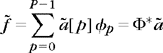
with decomposition coefficients ![]() that are a solution of a minimization problem that incorporates the precision parameter ε:
that are a solution of a minimization problem that incorporates the precision parameter ε:
In a denoising problem, f is replaced by the noisy signal X = f + W where W is the additive noise. It is then called a basis pursuit denoising algorithm.
Computing the solution of this quadratically constrained problem is more complicated than the linear programming problem corresponding to a basis pursuit. However, it can be recast as a second-order cone program, which is solved using interior point methods and, in particular, log-barrier methods [10] that extend the interior point algorithms for linear programming problems. These general-purpose algorithms can also be optimized to take into account the separability of the 11 norm. Iterative algorithms converging to the solution have also been developed [183].
The minimization problem (12.88) is convex and thus can also be solved through its Lagrangian formulation:
In the following, this Lagrangian minimization will be called a Lagrangian basis pursuit or l1 pursuit. For each ε > 0, there exists a Lagrangian multiplier T such that convex minimization (12.88) and the Lagrangian minimization (12.89) have a common solution [266, 463]. In a denoising problem, where f is replaced by X = f + W, it is easier to adjust T then ε to the noise level. Indeed, we shall see that a Lagrangian pursuit performs a generalized soft thresholding by T. For a Gaussian white noise σ, one can typically set T = λ σ with ![]() , where P is the dictionary size. Section 12.4.3 describes algorithms for computing a solution of the Lagrangian minimization (12.89).
, where P is the dictionary size. Section 12.4.3 describes algorithms for computing a solution of the Lagrangian minimization (12.89).
Figure 12.22 shows an example of basis pursuit denoising of an image contaminated by a Gaussian white noise. The dictionary includes a translation-invariant dyadic wavelet frame and a tight frame of local cosine vectors with a redundancy factor of 16. The resulting estimation is better than in a translation-invariant wavelet dictionary. Indeed, local cosine vectors provide more sparse representations of the image oscillatory textures.

FIGURE 12.22 (a) Original image f. (b) Noisy image X = f + W (SNR = 12.5 db). (c) Translation-invariant wavelet denoising, (SNR = 18.6 db). (d) Basis pursuit denoising in a dictionary that is a union of a translation-invariant wavelet frame and a frame of redundant local cosine vectors (SNR = 19.8 db).
Convexification of I0 with I1
Theorem 12.1 proves that a best M-term approximation fλT in a dictionary ![]() is obtained by minimizing the 10 Lagrangian (12.30)
is obtained by minimizing the 10 Lagrangian (12.30)
Since the 10 pseudo norm is not convex, Section 12.1.1 explains that the minimization of ![]() is intractable. An 10 norm can be approximated by an 1q pseudo-norm
is intractable. An 10 norm can be approximated by an 1q pseudo-norm

which is nonconvex for 0 ≤ q < 1, and convex and thus a norm for q ≥ 1. As q decreases, Figure 12.23 shows in P = 2 dimensions that the unit ball of vectors ![]() approaches the 10 unit “ball,” which corresponds to the two axes. The 11 Lagrangian minimization (12.89) can thus be interpreted as a convexification of the 10 Lagrangian minimization.
approaches the 10 unit “ball,” which corresponds to the two axes. The 11 Lagrangian minimization (12.89) can thus be interpreted as a convexification of the 10 Lagrangian minimization.

FIGURE 12.23 Unit balls of Iq functionals: (a) q = 0, (b) q = 0.5, (c) q = 1, (d) q = 1.5, and (e) q = 2.
Let ![]() be the support of the 11 Lagrangian pursuit solution
be the support of the 11 Lagrangian pursuit solution ![]() For
For ![]() , the support
, the support ![]() is typically not equal to the best M-term approximation support ΛT obtained by minimizing the 10 Lagrangian and
is typically not equal to the best M-term approximation support ΛT obtained by minimizing the 10 Lagrangian and ![]() . However, Section 12.5.3 proves that
. However, Section 12.5.3 proves that ![]() may include the main approximation vectors of ΛT and
may include the main approximation vectors of ΛT and ![]() can be of the same order as
can be of the same order as ![]() if ΛT satisfies an exact recovery condition that is specified.
if ΛT satisfies an exact recovery condition that is specified.
Generalized Soft Thresholding
A Lagrangian pursuit computes a sparse approximation ![]() of f by minimizing
of f by minimizing
Increasing T often reduces the support ![]() of
of ![]() but increases the approximation error
but increases the approximation error ![]() . The restriction of the dictionary operator and its adjoint to
. The restriction of the dictionary operator and its adjoint to ![]() is written as
is written as
Theorem 12.8, proved by Fuchs [266], gives necessary and sufficient conditions on ![]() and its support
and its support ![]() to be a minimizer of
to be a minimizer of ![]() .
.
Theorem 12.8: Fuchs. A vector ![]() is a minimum of
is a minimum of ![]() if and only if there exists
if and only if there exists ![]() such that
such that
There exists a solution ![]() with support
with support ![]() that corresponds to a family
that corresponds to a family ![]() of linearly independent dictionary vectors. The restriction
of linearly independent dictionary vectors. The restriction ![]() over its support satisfies
over its support satisfies
where ![]() is the pseudo inverse of
is the pseudo inverse of ![]() .
.
Proof.
If ![]() , then
, then ![]() is differentiable along the coordinate a[p] at the point
is differentiable along the coordinate a[p] at the point ![]() . Setting this derivative to 0 shows that
. Setting this derivative to 0 shows that ![]() is minimum if and only if
is minimum if and only if
If ![]() , let us consider the vector
, let us consider the vector ![]() . The corresponding Lagrangian value is
. The corresponding Lagrangian value is
By separately considering the cases τ > 0, and τ < 0, we verify that when τ goes to zero it implies that
Conditions (12.94) and (12.95) are equivalent to (12.92).
Conversely, if h satisfies (12.92), then for any a we verify that
Since ![]() is differentiable and convex, this leads to
is differentiable and convex, this leads to
because of (12.92), and thus ![]() minimizes
minimizes ![]() . The conditions (12.92) therefore are necessary and sufficient.
. The conditions (12.92) therefore are necessary and sufficient.
The proof of the existence of a solution ![]() corresponding to linear independent vectors
corresponding to linear independent vectors ![]() is identical to the proof of Theorem 12.7 in the basis pursuit context. Over the support
is identical to the proof of Theorem 12.7 in the basis pursuit context. Over the support ![]() , the necessary and sufficient condition (12.92) can be rewritten as
, the necessary and sufficient condition (12.92) can be rewritten as
which implies (12.93).
Let ![]() be the orthogonal projection of f over the space
be the orthogonal projection of f over the space ![]() generated by
generated by ![]() . Its coefficients are
. Its coefficients are ![]() Theorem 12.8 proves in (12.93) that
Theorem 12.8 proves in (12.93) that
which shows that the 11 minimization attenuates by an amount proportional to T the amplitude of the coefficients ![]() of the orthogonal projection
of the orthogonal projection ![]() . This can be interpreted as a generalized soft thresholding. If
. This can be interpreted as a generalized soft thresholding. If ![]() is an orthonormal basis, then ΦΦ* = Id and
is an orthonormal basis, then ΦΦ* = Id and ![]() is a classical soft thresholding of the coefficient Φf of f in this orthonormal basis.
is a classical soft thresholding of the coefficient Φf of f in this orthonormal basis.
Since ![]() , we know that
, we know that ![]() . Once the optimal Lagrangian support
. Once the optimal Lagrangian support ![]() is recovered, similar to the matching pursuit backprojection, the sparse approximation
is recovered, similar to the matching pursuit backprojection, the sparse approximation ![]() of f can be improved by computing the orthogonal projection
of f can be improved by computing the orthogonal projection ![]() and its coefficients
and its coefficients ![]() .
.
12.4.3 Computations of I1 Minimizations
The relaxed formulation of an 11 Lagrangian pursuit
cannot be formulated as a linear program, as opposed to the basis pursuit minimization (12.83). Several approaches have been developed to compute this minimization.
Iterative Thresholding
Several authors [100, 185, 196, 241, 255, 466] have proposed an iterative algorithm that solves (12.89) with a soft thresholding to decrease the 11 norm of the coefficients a, and a gradient descent to decrease the value of ![]() . The coefficient vector a may be complex, and
. The coefficient vector a may be complex, and ![]() is then the complex modulus.
is then the complex modulus.
1. Initialization. Choose a0 (e.g., 0), set k = 0, and compute b = Φf.
where ![]() .
.
4. Stop. If ![]() is smaller than a fixed-tolerance criterion, stop the iterations, otherwise set k ← k + 1 and go back to 2.
is smaller than a fixed-tolerance criterion, stop the iterations, otherwise set k ← k + 1 and go back to 2.
This algorithm includes the same gradient step as the Richardson iteration algorithm in Theorem 5.7, which inverts the symmetric operator L = ΦΦ*. The convergence condition ![]() is identical to the convergence condition (5.35) of the Richardson algorithm. Theorem 12.9 proves that the convergence is guaranteed for any a0.
is identical to the convergence condition (5.35) of the Richardson algorithm. Theorem 12.9 proves that the convergence is guaranteed for any a0.
Theorem 12.9.
converges to a solution of (12.89) for any a0 ∈ CP.
Proof.
The following proof is due to Daubechies, Defries, and DeMol [196], showing that ak converges to a minimum of the energy
for γ < ‖φφ*‖S−1. A proof of convergence for γ < 2 ‖φφ*‖S−1 can be found in [185].
To simplify notations, the dependencies of the Lagrangian on T and f are dropped, and it is written L1(a). Lemma 12.2 proves that ak+1 is the minimum of a modified surrogate Lagrangian L1(a, ak) that approximates L1(a) and depends on the previous iterate.
Lemma 12.2.
Let ξ be the operator that associates to a vector b the vector
For any b ∈ CN, ξ(b) is the unique minimizer of ![]() 1(a, b) over all a, where
1(a, b) over all a, where
Proof.
The modified Lagrangian ![]() is expanded as
is expanded as
where C1 and C2 are two constants that do not depend on a. This proves that ![]() 1(a, b) is a strictly convex function with respect to a. Since
1(a, b) is a strictly convex function with respect to a. Since
each term of this sum can be minimized independently, and Lemma 12.3 proves that the minimum is reached by ργT(b[p]). Moreover, at the minimum, the result (12.104) of Lemma 12.3 implies (12.103). Lemma 12.3 is proved by verifying (12.104) with a direct algebraic calculation.
Lemma 12.3.
The scalar energy e(α) = |β – α|2/2 + T|α| is minimized by α = ρT(β) and
We now prove that the ak defined in equation (12.100) converge to a fixed point of ξ, and that this fixed point is a minimizer of L1(a). The difficulty is that ξ is not strictly contracting. Without loss of generality, we assume that γ = 1 and that ‖φ*b‖ < ‖b‖. Otherwise, φ* is replaced by √γφ*, f by √γf, and T by γT. The thresholding operator ρT satisfies
This implies the contractions of the mapping ξ:
because ‖Φ*‖S < 1.
In the following, we write ![]() , which satisfies ‖La‖2 = ‖a‖2 – ‖Φ*a‖2. Lemma 12.2 shows that ak+1 is the minimizer of
, which satisfies ‖La‖2 = ‖a‖2 – ‖Φ*a‖2. Lemma 12.2 shows that ak+1 is the minimizer of ![]() , and thus
, and thus
so { L1(ak)}k is a nonincreasing sequence. Similarly,
so {L1(ak+1, ak)}k is also a nonincreasing sequence.
Since ‖Φ*‖S < 1, the operator L is positive definite, and if one denotes A > 0 the smallest eigenvalue of L,
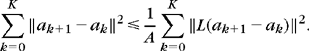
It results from (12.105) that 1/2‖L(ak+1 – ak)‖2 ≤ L1(ak) – L1(ak+1), and thus

It follows that the series σk ‖ak+1 – ak‖2 converges, and thus
the sequence {ak}k is bounded. As the vectors are in the finite-dimensional space CN, there exists a subsequence {aγ(k)}k that converges to some ã. Equation (12.106) proves that ξ(aγ(k)) also converges to ã, which is thus a fixed point of ξ.
The sequence {‖ak – ã‖}k is decreasing and thus convergent. But {‖aγ(k) – ã‖}k converges to 0 so the whole sequence ak is converging to ã.
Given that ξ(ã) = ã, Lemma 12.2 with γ = 1 proves that
which proves that L1(ã + h) ≥ L1(ã) + 1/2‖φ*h‖2, and thus ã is a minimizer of L1.
This theorem proves the convergence of the algorithm but provides no bound on the decay rate. It incorporates in the loop the Richardson gradient descent so its convergence is slower than the convergence of a Richardson inversion. Theorem 5.7 proves that this convergence depends on frame bounds. In this iterative thresholding algorithm, it depends on the frame bounds BΛ ≥ AΛ > 0 of the family of vectors {φp}p∈Λ over the support Λ of the solution as it evolves during the convergence. For a gradient descent alone, Theorem 5.7 proves that error decreases by a factor δ = max {|1 – γAΛ|, |1 – γBΛ|}. This factor is small if AΛ is small, which indicates that this family of vectors defines a nearly unstable frame. Once the final support A is recovered, the convergence is fast only if AΛ is also not too small. This property guarantees the numerical stability of the solution.
Backprojection
The amplitudes of the coefficients ![]() on the support
on the support ![]() are reduced relative to the coefficients
are reduced relative to the coefficients ![]() of the orthogonal projection
of the orthogonal projection ![]() of f on the space generated by
of f on the space generated by ![]() . The approximation error is reduced by a backprojection that recovers
. The approximation error is reduced by a backprojection that recovers ![]() from
from ![]() as in a matching pursuit.
as in a matching pursuit.
Implementing this backprojection with the Richardson algorithm is equivalent to continuing the iterations with the same gradient step (12.98) and by replacing the soft thresholding (12.99) by an orthogonal projector on ![]() :
:
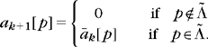 (12.107)
The convergence is then guaranteed by the Richardson theorem (5.7) and depends on ![]()
Automatic Threshold Updating
To solve the minimization under an error constraint of ε,
the Lagrange multiplier T must be adjusted to ε. A sequence of ![]() can be calculated so that
can be calculated so that ![]() converges to ε. The error
converges to ε. The error ![]() is an increasing function of Tl but not strictly. A possible threshold adjustment proposed by Chambolle [152] is
is an increasing function of Tl but not strictly. A possible threshold adjustment proposed by Chambolle [152] is
One can also update a threshold Tk with (12.109) at each step k of the soft-thresholding iteration, which works numerically well, although there is no proof of convergence.
Other Algorithms
Several types of algorithms can solve the 11 Lagrangian minimization (12.97). It includes primal-dual schemes [497], specialized interior points with preconditioned conjugate gradient [329], Bregman iterations [494], split Bregman iterations [275], two-step iterative thresholding [211], SGPL1 [104], gradient pursuit [115], gradient projection [256], fixed-point continuation [240], gradient methods [389, 390], coordinate-wise descent [261], and sequential subspace optimization [382].
Continuation methods like homotopy [228, 393] keep track of the solution ![]() of (12.97) for a decreasing sequence of thresholds Tl. For a given Tl, one can compute the next smallest Tl+1 where the support of the optimal solution includes a new component (or more rarely where a new component disappears) and the position of this component. At each iteration, the solution is then computed with the implicit equation (12.93) by calculating the pseudo inverse
of (12.97) for a decreasing sequence of thresholds Tl. For a given Tl, one can compute the next smallest Tl+1 where the support of the optimal solution includes a new component (or more rarely where a new component disappears) and the position of this component. At each iteration, the solution is then computed with the implicit equation (12.93) by calculating the pseudo inverse ![]() These algorithms are thus quite fast if the final solution
These algorithms are thus quite fast if the final solution ![]() is highly sparse, because only a few iterations are then necessary and the size of all matrices remains small.
is highly sparse, because only a few iterations are then necessary and the size of all matrices remains small.
It is difficult to compare all these algorithms because their speed of convergence depends on the sparsity of the solution and on the frame bounds of the dictionary vectors over the support solution. The iterative thresholding algorithm of Theorem 12.9 has the advantage of simplicity.
12.4.4 Sparse Synthesis versus Analysis and Total Variation Regularization
Matching pursuit and basis pursuit algorithms assume that the signal has a sparse synthesis in a dictionary ![]() and compute this representation with as few vectors as possible. The sparse synthesis hypothesis should not be confused with a sparse analysis hypothesis, which assumes that a linear signal transform
and compute this representation with as few vectors as possible. The sparse synthesis hypothesis should not be confused with a sparse analysis hypothesis, which assumes that a linear signal transform ![]() is sparse. A sparse analysis can often be related to some form of regularity of f. For example, piecewise regular signals have a sparse wavelet transform. Similarly, total variation regularizations make a sparse analysis assumption on the sparsity of the gradient vector field. Sparse analysis and synthesis assumptions are equivalent in an orthonormal basis, but are very different when the dictionary is redundant. These aspects are clarified and algorithms are provided to solve sparse analysis problems, including total variation regularizations.
is sparse. A sparse analysis can often be related to some form of regularity of f. For example, piecewise regular signals have a sparse wavelet transform. Similarly, total variation regularizations make a sparse analysis assumption on the sparsity of the gradient vector field. Sparse analysis and synthesis assumptions are equivalent in an orthonormal basis, but are very different when the dictionary is redundant. These aspects are clarified and algorithms are provided to solve sparse analysis problems, including total variation regularizations.
Sparse Synthesis and Analysis with I1 Norms
A basis pursuit incorporates the sparse synthesis assumption by minimizing the 11 norm of the synthesis coefficients. To approximate f, the Lagrangian formulation computes
In a denoising problem, f is replaced by the input noisy signal X = f + W, and if W is a Gaussian white noise of variance σ2, then T is proportional to σ
A sparse analysis approximation of f computes
where ε is the approximation precision. This problem is convex. Similarly, in a denoising problem, f is replaced by the input noisy signal X = f + W. A solution ![]() of (12.111) can be computed as a solution of the Lagrangian formulation
of (12.111) can be computed as a solution of the Lagrangian formulation
where T depends on ε. In a denoising problem, f is also replaced by the noisy signal X = f + W, and T is proportional to the noise standard deviation σ
If D is an orthonormal basis, then ![]() so
so ![]() . The analysis and synthesis prior assumptions are then equivalent. This is, however, not the case when the dictionaries are redundant [243]. In a redundant dictionary, a sparse synthesis assumes that a signal is well approximated by few well-chosen dictionary vectors. However, it often has a nonsparse representation with badly chosen dictionary vectors. For example, a high-frequency oscillatory texture has a sparse synthesis in a dictionary of wavelet and local cosine because it is well represented by local cosine vectors, but it does not have a sparse analysis representation in this dictionary because the wavelet coefficients of these textures are not sparse.
. The analysis and synthesis prior assumptions are then equivalent. This is, however, not the case when the dictionaries are redundant [243]. In a redundant dictionary, a sparse synthesis assumes that a signal is well approximated by few well-chosen dictionary vectors. However, it often has a nonsparse representation with badly chosen dictionary vectors. For example, a high-frequency oscillatory texture has a sparse synthesis in a dictionary of wavelet and local cosine because it is well represented by local cosine vectors, but it does not have a sparse analysis representation in this dictionary because the wavelet coefficients of these textures are not sparse.
Thresholding algorithms in redundant translation-invariant dictionaries such as translation-invariant wavelet frames rely on a sparse analysis assumption. They select all large frame coefficients, and the estimation is precise if there are relatively few of them. Sparse analysis constraints can often be interpreted as imposing some form of signal regularity condition—for example, with a total variation norm.
In Section 12.4.3 we describe an iterative thresholding that solves the sparse synthesis Lagrangian minimization (12.110). When the dictionary is redundant, the sparse analysis minimization (12.112) must integrate that the 11 norm is carried over a redundant set of coefficients a[p] = φh[p] that cannot be adjusted independently. If φ is a frame, then Theorem 5.9 proves that a satisfies a reproducing kernel equation a = φφ+a where φφ+ is an orthogonal projector on the space of frame coefficients. One could think of solving (12.112) with the iterative soft-thresholding algorithm that minimizes (12.110), and project with the projector φφ+a at each iteration on the constraints, but this algorithm is not guaranteed to converge.
Total Variation Denoising
Rudin, Osher, and Fatemi’s [420] total variation regularization algorithm assumes that the image gradient ![]() is sparse, which is enforced by minimizing its L1 norm, and thus the total image variation
is sparse, which is enforced by minimizing its L1 norm, and thus the total image variation ![]() . Over discrete images, the gradient vector is computed with horizontal and vertical finite differences. Let τ1 = (1, 0) and τ2 = (0, 1):
. Over discrete images, the gradient vector is computed with horizontal and vertical finite differences. Let τ1 = (1, 0) and τ2 = (0, 1):
The discrete total variation norm is the complex l1 norm
where Φ is a complex valued analysis operator
The discrete image gradient Φf = D1f + iD2f has the same size N as the image but has twice the scalar values because of the two partial derivative coordinates. Thus, it defines a redundant representation in RN. The finite difference D1 and D2 are convolution operators with transfer functions that vanish at the 0 frequency. As a result, Φ is not a frame of RN. However, it is invertible on the subspace ![]() of dimension N – 1. Since we are in finite dimension, it defines a frame of V, but the pseudo inverse Φ+ in (5.21) becomes numerically unstable when N increases because the frame bound ratio A/B tends to zero. Theorem 5.9 proves that ΦΦ+ remains an orthogonal projector on the space of gradient coefficients.
of dimension N – 1. Since we are in finite dimension, it defines a frame of V, but the pseudo inverse Φ+ in (5.21) becomes numerically unstable when N increases because the frame bound ratio A/B tends to zero. Theorem 5.9 proves that ΦΦ+ remains an orthogonal projector on the space of gradient coefficients.
Figure 12.24 shows an example of image denoising with a total variation regularization. The total variation minimization recovers an image with a gradient vector that is as sparse as possible, which has a tendency to produce piecewise constant regions when the thresholding increases. As a result, the total variation image denoising most often yields a smaller SNR than wavelet thresholding estimators, unless the image is piecewise constant.
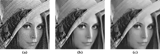
Computation of Sparse Analysis Approximations and Denoising with 11 Norms
A sparse analysis approximation is defined by
and f is replaced by the noisy data X = f + W in a denoising problem. Chambolle [152] sets a dual problem by verifying that the regularization term ![]() can be replaced by a set of dual variables:
can be replaced by a set of dual variables:
with ![]() , and where
, and where ![]() is the modulus of complex numbers. Because of (12.114), the regularization
is the modulus of complex numbers. Because of (12.114), the regularization ![]() is “linearized” by taking a maximum over inner products with vectors in a convex set r ∈ κ This decomposition remains valid for any positively homogeneous functional J, which satisfies J(Λh) = |λ|J(h).
is “linearized” by taking a maximum over inner products with vectors in a convex set r ∈ κ This decomposition remains valid for any positively homogeneous functional J, which satisfies J(Λh) = |λ|J(h).
The minimization (12.113) is thus rewritten as a minimization and maximization:
Inverting the min and max and computing the solution of the min problem shows that ![]() is written as
is written as
which means that ![]() is the projection of f/T on the convex set κ
is the projection of f/T on the convex set κ
The solution of (12.113) is thus also the solution of the following convex problem:
The solution ![]() is not necessarily unique, but both
is not necessarily unique, but both ![]() and
and ![]() are unique. With this dual formulation, the redundancy of a = Φf in the 11 norm of (12.113) does not appear anymore.
are unique. With this dual formulation, the redundancy of a = Φf in the 11 norm of (12.113) does not appear anymore.
Starting from a choice of a0, for example a0 = 0, Chambolle [152] computes ![]() by iterating between a gradient step to minimize
by iterating between a gradient step to minimize ![]() ,
,
and a “projection” step to ensure that ![]() for all p. An orthogonal projection at each iteration on the constraint gives
for all p. An orthogonal projection at each iteration on the constraint gives
One can verify [152] that the convergence is guaranteed if ![]() . To satisfy the constraints, another possibility is to set
. To satisfy the constraints, another possibility is to set
For the gradient operator ![]() discretized with finite differences in 2D,
discretized with finite differences in 2D, ![]() so one can choose γ = 1/4. The convergence is often fast during the first few iterations, leading to a visually satisfying result, but the remaining iterations tend to converge slowly to the final solution.
so one can choose γ = 1/4. The convergence is often fast during the first few iterations, leading to a visually satisfying result, but the remaining iterations tend to converge slowly to the final solution.
Other iterative algorithms have been proposed to solve (12.113), for instance, fixed-point iterations [476], second-order cone programming [274], splitting [480], splitting with Bregman iterations [275], and primal-dual methods [153, 497]. Primal-dual methods tend to have a faster convergence than the Chambolle algorithm.
Chambolle [152] proves that the sparse analysis minimization (12.111) with a precision ε is obtained by iteratively computing the solution ![]() of Lagrangian problems (12.113) for thresholds Tl that are adjusted with
of Lagrangian problems (12.113) for thresholds Tl that are adjusted with
The convergence proof relies on the fact that ![]() is a strictly increasing function of T for the analysis problem, which is not true for the synthesis problem.
is a strictly increasing function of T for the analysis problem, which is not true for the synthesis problem.
Computation of Sparse Analysis Inverse Problems with l1 Norms
In inverse problems studied in Chapter 13, f is estimated from Y = Uf + W, where U is a linear operator and W an additive noise. A sparse analysis estimation of f computes
The sparse Lagrangian analysis approximation operator ST in (12.113) can be used to replace the wavelet soft thresholding in the iterative thresholding algorithm (12.100), which leads to the iteration
One can prove with the general machinery of proximal iterations that ![]() converges to a solution
converges to a solution ![]() of (12.118) if
of (12.118) if ![]() [186]. The algorithm is implemented with two embedded loops. The outer loop on k computes
[186]. The algorithm is implemented with two embedded loops. The outer loop on k computes ![]() , followed by the inner loop, which computes the Lagrangian approximation ST, for example, with Chambolle algorithm.
, followed by the inner loop, which computes the Lagrangian approximation ST, for example, with Chambolle algorithm.