
7.4 BIORTHOGONAL WAVELET BASES
The stability and completeness properties of biorthogonal wavelet bases are described for perfect reconstruction filters h and ![]() having a finite impulse response. The design of linear phase wavelets with compact support is explained in Section 7.4.2.
having a finite impulse response. The design of linear phase wavelets with compact support is explained in Section 7.4.2.
7.4.1 Construction of Biorthogonal Wavelet Bases
An infinite cascade of perfect reconstruction filters (h, g) and (![]() ,
, ![]() ) yields two scaling functions and wavelets having a Fourier transform that satisfies
) yields two scaling functions and wavelets having a Fourier transform that satisfies
In the time domain, these relations become
The perfect reconstruction conditions are given by Theorem 7.12. If we normalize the gain and shift to a = 1 and l = 0, the filters must satisfy
Wavelets should have a zero average, which means that ![]() . This is obtained by setting
. This is obtained by setting ![]() and thus
and thus ![]() . The perfect reconstruction condition (7.146) implies that
. The perfect reconstruction condition (7.146) implies that ![]() . Since both filters are defined up to multiplicative constants equal to Λ and Λ−1, respectively, we adjust λ so that
. Since both filters are defined up to multiplicative constants equal to Λ and Λ−1, respectively, we adjust λ so that ![]() .
.
In the following, we also suppose that h and ![]() are finite impulse-response filters. One can then prove [19] that
are finite impulse-response filters. One can then prove [19] that
 (7.148)
are the Fourier transforms of distributions of compact support. However, these distributions may exhibit wild behavior and have infinite energy. Some further conditions must be imposed to guarantee that ![]() and
and ![]() are the Fourier transforms of finite energy functions. Theorem 7.14 gives sufficient conditions on the perfect reconstruction filters for synthesizing biorthogonal wavelet bases of L2(
are the Fourier transforms of finite energy functions. Theorem 7.14 gives sufficient conditions on the perfect reconstruction filters for synthesizing biorthogonal wavelet bases of L2(![]() ).
).
Theorem 7.14:
Cohen, Daubechies, Feauveau. Suppose that there exist strictly positive trigonometric polynomials P(eiω) and ![]() (eiω) such that
(eiω) such that
and that P and ![]() are unique (up to normalization). Suppose that
are unique (up to normalization). Suppose that
Then, the functions ![]() and
and ![]() defined in (7.148) belong to L2(
defined in (7.148) belong to L2(![]() ), and ϕ,
), and ϕ, ![]() satisfy biorthogonal relations
satisfy biorthogonal relations
The two wavelet families ![]() and
and ![]() are biorthogonal Riesz bases of L2(
are biorthogonal Riesz bases of L2(![]() ).
).
The proof of this theorem is in [172] and [19]. The hypothesis (7.151) is also imposed by Theorem 7.2, which constructs orthogonal bases of scaling functions. The conditions (7.149) and (7.150) do not appear in the construction of wavelet orthogonal bases because they are always satisfied with P(eiω) = ![]() (eiω) = 1, and one can prove that constants are the only invariant trigonometric polynomials [341].
(eiω) = 1, and one can prove that constants are the only invariant trigonometric polynomials [341].
Biorthogonality means that for any (j, j′, n, n′) ∈![]() 4,
4,
Any f ∈L2(![]() ) has two possible decompositions in these bases:
) has two possible decompositions in these bases:
 (7.154)
The Riesz stability implies that there exist A > 0 and B > 0 such that
 (7.155)
 (7.156)
Multiresolutions
Biorthogonal wavelet bases are related to multiresolution approximations. The family {ϕ(t – n)}n∈![]() is a Riesz basis of the space V0 it generates, whereas
is a Riesz basis of the space V0 it generates, whereas ![]() is a Riesz basis of another space
is a Riesz basis of another space ![]() 0. Let Vj and
0. Let Vj and ![]() j be the spaces defined by
j be the spaces defined by
One can verify that {Vj}j∈![]() and {
and {![]() j}j∈
j}j∈![]() are two multiresolution approximations of L2(
are two multiresolution approximations of L2(![]() ). For any j ∈
). For any j ∈ ![]() , {ϕj, n}n∈
, {ϕj, n}n∈![]() and
and ![]() are Riesz bases of Vj and
are Riesz bases of Vj and ![]() j. The dilated wavelets {ψj, n}n∈
j. The dilated wavelets {ψj, n}n∈![]() and
and ![]() are bases of two detail spaces Wj and
are bases of two detail spaces Wj and ![]() j such that
j such that
The biorthogonality of the decomposition and reconstruction wavelets implies that Wj is not orthogonal to Vj but is to ![]() j, whereas
j, whereas ![]() j is not orthogonal to
j is not orthogonal to ![]() j but is to Vj.
j but is to Vj.
Fast Biorthogonal Wavelet Transform
The perfect reconstruction filter bank discussed in Section 7.3.2 implements a fast biorthogonal wavelet transform. For any discrete signal input b[n] sampled at intervals N−1 = 2L, there exists f ∈ VL such that aL[n] = 〈f, ϕL, n〉 = N−1/2 b[n]. The wavelet coefficients are computed by successive convolutions with ![]() and
and ![]() .
.
Let aj[n] = 〈f, ϕj, n〉 and dj[n] = 〈f, ψj, n〉. As in Theorem 7.10, one can prove that
The reconstruction is performed with the dual filters ![]() and
and ![]() :
:
If aL includes N nonzero samples, the biorthogonal wavelet representation [{dj}L < j ≤ J, aJ] is calculated with O(N) operations by iterating (7.157) for L ≤ j < J. The reconstruction of aL by applying (7.158) for J > j ≥ L requires the same number of operations.
7.4.2 Biorthogonal Wavelet Design
The support size, the number of vanishing moments, the regularity, wavelet ordering, and the symmetry of biorthogonal wavelets is controlled with an appropriate design of h and ![]() .
.
Support
If the perfect reconstruction filters h and ![]() have a finite impulse response, then the corresponding scaling functions and wavelets also have a compact support. As in Section 7.2.1, one can show that if h[n] and
have a finite impulse response, then the corresponding scaling functions and wavelets also have a compact support. As in Section 7.2.1, one can show that if h[n] and ![]() [n] are nonzero, respectively, for N1 ≤ n ≤ N2 and
[n] are nonzero, respectively, for N1 ≤ n ≤ N2 and ![]() 1 ≤ n ≤
1 ≤ n ≤ ![]() 2, then ϕ and
2, then ϕ and ![]() have a support equal to [N1, N2] and [
have a support equal to [N1, N2] and [![]() 1,
1, ![]() 2], respectively. Since
2], respectively. Since
the supports of ψ and ![]() defined in (7.145) are, respectively,
defined in (7.145) are, respectively,
 (7.159)
Thus, both wavelets have a support of the same size and equal to
Vanishing Moments
The number of vanishing moments of ψ and ![]() depends on the number of zeroes at ω = π of ĥ(ω) and
depends on the number of zeroes at ω = π of ĥ(ω) and ![]() . Theorem 7.4 proves that ψ has
. Theorem 7.4 proves that ψ has ![]() vanishing moments if the derivatives of its Fourier transform satisfy
vanishing moments if the derivatives of its Fourier transform satisfy ![]() for k ≤
for k ≤ ![]() . Since
. Since ![]() , (7.41) implies that it is equivalent to impose that
, (7.41) implies that it is equivalent to impose that ![]() has a zero of order
has a zero of order ![]() at ω = 0. Since
at ω = 0. Since ![]() , this means that
, this means that ![]() (ω) has a zero of order
(ω) has a zero of order ![]() at ω = π. Similarly, the number of vanishing moments of
at ω = π. Similarly, the number of vanishing moments of ![]() is equal to the number p of zeroes of ĥ(ω) at π.
is equal to the number p of zeroes of ĥ(ω) at π.
Regularity
Although the regularity of a function is a priori independent of the number of vanishing moments, the smoothness of biorthogonal wavelets is related to their vanishing moments. The regularity of ϕ and ψ is the same because (7.145) shows that ψ is a finite linear expansion of ϕ translated. Tchamitchian’s theorem (7.6) gives a sufficient condition for estimating this regularity. If ĥ(ω) has a zero of order p at π, we can perform the factorization
Let ![]() . Theorem 7.6 proves that ϕ is uniformly Lipschitz α for
. Theorem 7.6 proves that ϕ is uniformly Lipschitz α for
Generally, log2 B increases more slowly than p. This implies that the regularity of ϕ and ψ increases with p, which is equal to the number of vanishing moments of ![]() . Similarly, one can show that the regularity of
. Similarly, one can show that the regularity of ![]() and
and ![]() increases with
increases with ![]() , which is the number of vanishing moments of ψ. If ĥ and
, which is the number of vanishing moments of ψ. If ĥ and ![]() have different numbers of zeroes at π, the properties of ψ and
have different numbers of zeroes at π, the properties of ψ and ![]() can be very different.
can be very different.
Ordering of Wavelets
Since ψ and ![]() might not have the same regularity and number of vanishing moments, the two reconstruction formulas
might not have the same regularity and number of vanishing moments, the two reconstruction formulas
 (7.162)
 (7.163)
are not equivalent. The decomposition (7.162) is obtained with the filters (h, g), and the reconstruction with (![]() ,
, ![]() ). The inverse formula (7.163) corresponds to (
). The inverse formula (7.163) corresponds to (![]() ,
, ![]() ) at the decomposition and (h, g) at the reconstruction.
) at the decomposition and (h, g) at the reconstruction.
To produce small wavelet coefficients in regular regions we must compute the inner products using the wavelet with the maximum number of vanishing moments. The reconstruction is then performed with the other wavelet, which is generally the smoothest one. If errors are added to the wavelet coefficients, for example with a quantization, a smooth wavelet at the reconstruction introduces a smooth error. The number of vanishing moments of ψ is equal to the number ![]() of zeroes at π of
of zeroes at π of ![]() . Increasing
. Increasing ![]() also increases the regularity of
also increases the regularity of ![]() . Thus, it is better to use h at the decomposition and
. Thus, it is better to use h at the decomposition and ![]() at the reconstruction if ĥ has fewer zeroes at π than
at the reconstruction if ĥ has fewer zeroes at π than ![]() .
.
Symmetry
It is possible to construct smooth biorthogonal wavelets of compact support that are either symmetric or antisymmetric. This is impossible for orthogonal wavelets, besides the particular case of the Haar basis. Symmetric or antisymmetric wavelets are synthesized with perfect reconstruction filters having a linear phase. If h and ![]() have an odd number of nonzero samples and are symmetric about n = 0, the reader can verify that ϕ and
have an odd number of nonzero samples and are symmetric about n = 0, the reader can verify that ϕ and ![]() are symmetric about t = 0, while ψ and
are symmetric about t = 0, while ψ and ![]() are symmetric with respect to a shifted center. If h and
are symmetric with respect to a shifted center. If h and ![]() have an even number of nonzero samples and are symmetric about n = 1/2, then ϕ(t) and
have an even number of nonzero samples and are symmetric about n = 1/2, then ϕ(t) and ![]() are symmetric about t = 1/2, while ψ and
are symmetric about t = 1/2, while ψ and ![]() are antisymmetric with respect to a shifted center. When the wavelets are symmetric or antisymmetric, wavelet bases over finite intervals are constructed with the folding procedure of Section 7.5.2.
are antisymmetric with respect to a shifted center. When the wavelets are symmetric or antisymmetric, wavelet bases over finite intervals are constructed with the folding procedure of Section 7.5.2.
7.4.3 Compactly Supported Biorthogonal Wavelets
We study the design of biorthogonal wavelets with a minimum-size support for a specified number of vanishing moments. Symmetric or antisymmetric compactly supported spline biorthogonal wavelet bases are constructed with a technique introduced in [172].
Theorem 7.15:
Cohen, Daubechies, Feauveau. Biorthogonal wavelets ψ and ![]() with, respectively,
with, respectively, ![]() and p vanishing moments have a support size of at least p +
and p vanishing moments have a support size of at least p + ![]() − 1. CDF biorthogonal wavelets have a minimum support size p +
− 1. CDF biorthogonal wavelets have a minimum support size p + ![]() − 1.
− 1.
Proof.
The proof follows the same approach as the proof of Daubechies’ theorem (7.7). One can verify that p and ![]() must necessarily have the same parity. We concentrate on filters h[n] and h[n] that have a symmetry with respect to n = 0 or n = 1/2. The general case proceeds similarly. We can then factor
must necessarily have the same parity. We concentrate on filters h[n] and h[n] that have a symmetry with respect to n = 0 or n = 1/2. The general case proceeds similarly. We can then factor
with ε = 0 for p and ![]() for even values and ε = 1 for odd values. Let q = (p +
for even values and ε = 1 for odd values. Let q = (p + ![]() )/2. The perfect reconstruction condition
)/2. The perfect reconstruction condition
where the polynomial P(y) must satisfy for all y ∈[0, 1]
We saw in (7.96) that the polynomial of minimum degree satisfying this equation is
 (7.168)
The spectral factorization (7.166) is solved with a root attribution similar to (7.98). The resulting minimum support of ψ and ![]() specified by (7.160) is then p +
specified by (7.160) is then p +![]() − 1.
− 1.
Spline Biorthogonal Wavelets
with ε = 0 for p even and ε = 1 for p odd. The scaling function computed with (7.148) is then a box spline of degree p − 1:
Since ψ is a linear combination of box splines ϕ (2t – n), it is a compactly supported polynomial spline of the same degree.
The number of vanishing moments ![]() of ψ is a free parameter, which must have the same parity as p. Let q = (p + p)/2. The biorthogonal filter
of ψ is a free parameter, which must have the same parity as p. Let q = (p + p)/2. The biorthogonal filter  of minimum length is obtained by observing that L(cos ω) = 1 in (7.164). Thus, the factorization (7.166) and (7.168) imply that
These filters satisfy the conditions of Theorem 7.14 and therefore generate biorthogonal wavelet bases. Table 7.3 gives the filter coefficients for (p = 2, ![]() = 4) and (p = 3,
= 4) and (p = 3, ![]() = 7); see Figure 7.14 for the resulting dual wavelet and scaling functions.
= 7); see Figure 7.14 for the resulting dual wavelet and scaling functions.
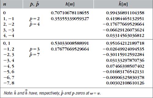
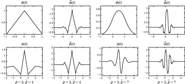
FIGURE 7.14 Spline biorthogonal wavelets and scaling functions of compact support corresponding to Table 7.3 filters.
Closer Filter Length
Biorthogonal filters h and ![]() of more similar length are obtained by factoring the polynomial
of more similar length are obtained by factoring the polynomial ![]() in (7.166) with two polynomial L(cos ω) and
in (7.166) with two polynomial L(cos ω) and ![]() (cos ω) of similar degree. There is a limited number of possible factorizations. For q = (p +
(cos ω) of similar degree. There is a limited number of possible factorizations. For q = (p + ![]() )/2 < 4, the only solution is L(cos ω) = 1. For q = 4 there is one nontrivial factorization, and for q = 5 there are two. Table 7.4 gives the resulting coefficients of the filters h and
)/2 < 4, the only solution is L(cos ω) = 1. For q = 4 there is one nontrivial factorization, and for q = 5 there are two. Table 7.4 gives the resulting coefficients of the filters h and ![]() of most similar length, computed by Cohen, Daubechies, and Feauveau [172]. These filters also satisfy the conditions of Theorem 7.14 and therefore define biorthogonal wavelet bases.
of most similar length, computed by Cohen, Daubechies, and Feauveau [172]. These filters also satisfy the conditions of Theorem 7.14 and therefore define biorthogonal wavelet bases.
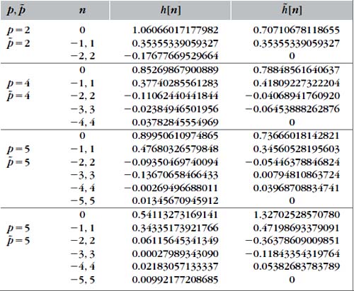
Figure 7.15 gives the scaling functions and wavelets for p = ![]() = 2 and p =
= 2 and p = ![]() = 4, which correspond to filter sizes 5/3 and 9/7, respectively. For p = p = 4, ϕ, ψ are similar to
= 4, which correspond to filter sizes 5/3 and 9/7, respectively. For p = p = 4, ϕ, ψ are similar to ![]() , which indicates that this basis is nearly orthogonal. This particular set of filters is often used in image compression and recommended for JPEG-2000. The quasi-orthogonality guarantees a good numerical stability and the symmetry allows one to use the folding procedure of Section 7.5.2 at the boundaries. There are also enough vanishing moments to create small wavelet coefficients in regular image domains. Section 7.8.5 describes their lifting implementation, which is simple and efficient. Filter sizes 5/3 are also recommended for lossless compression with JPEG-2000, because they use integer operations with a lifting algorithm. The design of other compactly supported biorthogonal filters is discussed extensively in [172, 473].
, which indicates that this basis is nearly orthogonal. This particular set of filters is often used in image compression and recommended for JPEG-2000. The quasi-orthogonality guarantees a good numerical stability and the symmetry allows one to use the folding procedure of Section 7.5.2 at the boundaries. There are also enough vanishing moments to create small wavelet coefficients in regular image domains. Section 7.8.5 describes their lifting implementation, which is simple and efficient. Filter sizes 5/3 are also recommended for lossless compression with JPEG-2000, because they use integer operations with a lifting algorithm. The design of other compactly supported biorthogonal filters is discussed extensively in [172, 473].
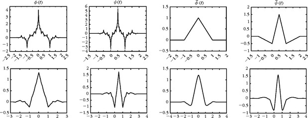
FIGURE 7.15 Biorthogonal wavelets and scaling functions calculated with the filters of Table 7.4, with p = 2 and ![]() = 2 (top row) and p = 4 and p = 4 (bottom row).
= 2 (top row) and p = 4 and p = 4 (bottom row).
7.5 WAVELET BASES ON AN INTERVAL
To decompose signals f defined over an interval [0, 1], it is necessary to construct wavelet bases of L2[0, 1]. Such bases are synthesized by modifying the wavelets ψj, n(t) = 2−j/2ψ(2−j t – n) of a basis ![]() of L2(
of L2(![]() ). Inside wavelets ψj, n, have a support included in [0, 1], and are not modified. Boundary wavelets ψj, n, have a support that overlaps t = 0 or t = 1, and are transformed into functions having a support in [0, 1], which are designed in order to provide the necessary complement to generate a basis of L2 [0, 1]. If ψ has a compact support, then there is a constant number of boundary wavelets at each scale.
). Inside wavelets ψj, n, have a support included in [0, 1], and are not modified. Boundary wavelets ψj, n, have a support that overlaps t = 0 or t = 1, and are transformed into functions having a support in [0, 1], which are designed in order to provide the necessary complement to generate a basis of L2 [0, 1]. If ψ has a compact support, then there is a constant number of boundary wavelets at each scale.
The main difficulty is to construct boundary wavelets that keep their vanishing moments. The next three sections describe different approaches to constructing boundary wavelets. Periodic wavelets have no vanishing moments at the boundary, whereas folded wavelets have one vanishing moment. The custom-designed boundary wavelets of Section 7.5.3 have as many vanishing moments as the inside wavelets but are more complicated to construct. Scaling functions ϕj, n are also restricted to [0, 1] by modifying the scaling functions ![]() associated with the wavelets ψj, n. The resulting wavelet basis of L2[0, 1] is composed of 2−J scaling functions at a coarse scale 2J < 1, plus 2−j wavelets at each scale 2j ≤ 2J:
associated with the wavelets ψj, n. The resulting wavelet basis of L2[0, 1] is composed of 2−J scaling functions at a coarse scale 2J < 1, plus 2−j wavelets at each scale 2j ≤ 2J:
On any interval [a, b], a wavelet orthonormal basis of L2[a, b] is constructed with a dilation by b – a and a translation by a of the wavelets in (7.171).
Discrete Basis of  N
N
The decomposition of a signal in a wavelet basis over an interval is computed by modifying the fast wavelet transform algorithm of Section 7.3.1. A discrete signal b[n] of N samples is associated to the approximation of a signal f ∈ L2[0, 1] at a scale N−1 = 2L with (7.111):
Its wavelet coefficients can be calculated at scales 1 ≥ 2j > 2L. We set
The wavelets and scaling functions with support inside [0, 1] are identical to the wavelets and scaling functions of a basis of L2(![]() ). Thus, the corresponding coefficients aj[n] and dj[n] can be calculated with the decomposition and reconstruction equations given by Theorem 7.10. However, these convolution formulas must be modified near the boundary where the wavelets and scaling functions are modified. Boundary calculations depend on the specific design of the boundary wavelets, as explained in the next three sections. The resulting filter bank algorithm still computes the N coefficients of the wavelet representation [aJ, {dj}L<j≤J] of aL with O(N) operations.
). Thus, the corresponding coefficients aj[n] and dj[n] can be calculated with the decomposition and reconstruction equations given by Theorem 7.10. However, these convolution formulas must be modified near the boundary where the wavelets and scaling functions are modified. Boundary calculations depend on the specific design of the boundary wavelets, as explained in the next three sections. The resulting filter bank algorithm still computes the N coefficients of the wavelet representation [aJ, {dj}L<j≤J] of aL with O(N) operations.
Wavelet coefficients can also be written as discrete inner products of aL with discrete wavelets:
As in Section 7.3.3, we verify that
7.5.1 Periodic Wavelets
A wavelet basis ![]() of L2(
of L2(![]() ) is transformed into a wavelet basis of L2[0, 1] by periodizing each ψj, n. The periodization of f ∈L2(
) is transformed into a wavelet basis of L2[0, 1] by periodizing each ψj, n. The periodization of f ∈L2(![]() ) over [0, 1] is defined by
) over [0, 1] is defined by
 (7.174)
The resulting periodic wavelets are
For j ≤ 0, there are 2−j different ψpérj, n indexed by 0 ≤ n < 2−j. If the support of ψj, n is included in [0, 1], then ![]() for t ∈[0, 1]. Thus, the restriction to [0, 1] of this periodization modifies only the boundary wavelets with a support that overlaps t = 0 or t = 1.
for t ∈[0, 1]. Thus, the restriction to [0, 1] of this periodization modifies only the boundary wavelets with a support that overlaps t = 0 or t = 1.
As indicated in Figure 7.16, such wavelets are transformed into boundary wavelets that have two disjoint components near t = 0 and t = 1. Taken separately, the components near t = 0 and t = 1 of these boundary wavelets have no vanishing moments, and thus create large signal coefficients, as we shall see later. Theorem 7.16 proves that periodic wavelets together with periodized scaling functions φpérj, n generate an orthogonal basis of L2[0, 1].

FIGURE 7.16 The restriction to [0, 1] of a periodic wavelet ψpérj, n has two disjoint components near t = 0 and t = 1.
Lemma 7.2.
Let α(t), β(t) ∈ L2(![]() ). If 〈α(t), β(t + k)〉 = 0 for all k ∈
). If 〈α(t), β(t + k)〉 = 0 for all k ∈ ![]() , then
, then
To verify (7.176) we insert the definition (7.174) of periodized functions:
Since ![]() is orthogonal in L2(
is orthogonal in L2(![]() ), we can verify that any two different wavelets or scaling functions αpér and βpér in (7.175) have necessarily a nonperiodized version that satisfies 〈α(t), β(t + k)〉 = 0 for all k ∈
), we can verify that any two different wavelets or scaling functions αpér and βpér in (7.175) have necessarily a nonperiodized version that satisfies 〈α(t), β(t + k)〉 = 0 for all k ∈ ![]() . Thus, this lemma proves that (7.175) is orthogonal in L2[0, 1].
. Thus, this lemma proves that (7.175) is orthogonal in L2[0, 1].
To prove that this family generates L2[0, 1], we extend f ∈ L2[0, 1] with zeros outside [0, 1] and decompose it in the wavelet basis of L2(![]() ):
):
 (7.177)
This zero extension is periodized with the sum (7.174), which defines fpér(t) = f (t) for t ∈ [0, 1]. Periodizing (7.177) proves that f can be decomposed over the periodized wavelet family (7.175) in L2[0, 1].
Theorem 7.16 shows that periodizing a wavelet orthogonal basis of L2(![]() ) defines a wavelet orthogonal basis of L2[0, 1]. If J = 0, then there is a single scaling function, and one can verify that ϕ0,0(t) = 1. The resulting scaling coefficient 〈f, ϕ0,0〉 is the average of f over [0, 1].
) defines a wavelet orthogonal basis of L2[0, 1]. If J = 0, then there is a single scaling function, and one can verify that ϕ0,0(t) = 1. The resulting scaling coefficient 〈f, ϕ0,0〉 is the average of f over [0, 1].
Periodic wavelet bases have the disadvantage of creating high-amplitude wavelet coefficients in the neighborhood of t = 0 and t = 1, because the boundary wavelets have separate components with no vanishing moments. If f (0) ≠ f (1), the wavelet coefficients behave as if the signal were discontinuous at the boundaries. This can also be verified by extending f ∈ L2[0, 1] into an infinite 1 periodic signal fpér and by showing that
If f (0) ≠ f (1), then fpér (t) is discontinuous at t = 0 and t = 1, which creates high-amplitude wavelet coefficients when ψj, n overlaps the interval boundaries.
Periodic Discrete Transform
For f ∈ L2[0, 1] let us consider
We verify as in (7.178) that these inner products are equal to the coefficients of a periodic signal decomposed in a nonperiodic wavelet basis:
Thus, the convolution formulas of Theorem 7.10 apply if we take into account the periodicity of fpér. This means that aj[n] and dj[n] are considered as discrete signals of period 2−j, and all convolutions in (7.102-7.104) must therefore be replaced by circular convolutions. Despite the poor behavior of periodic wavelets near the boundaries, they are often used because the numerical implementation is particularly simple.
7.5.2 Folded Wavelets
Decomposing f ∈ L2[0, 1] in a periodic wavelet basis was shown in (7.178) to be equivalent to a decomposition of fpér in a regular basis of L2(![]() ). Let us extend f with zeros outside [0, 1]. To avoid creating discontinuities with such a periodization, the signal is folded with respect to t = 0: f0(t) = f (t) + f (–t). The support of f0 is [–1, 1] and it is transformed into a 2 periodic signal, as illustrated in Figure 7.17:
). Let us extend f with zeros outside [0, 1]. To avoid creating discontinuities with such a periodization, the signal is folded with respect to t = 0: f0(t) = f (t) + f (–t). The support of f0 is [–1, 1] and it is transformed into a 2 periodic signal, as illustrated in Figure 7.17:
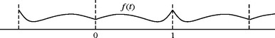
FIGURE 7.17 The folded signal frepl(t) is 2 periodic, symmetric about t = 0 and t = 1, and equal to f(t) on [0, 1].
 (7.179)
Clearly frepl (t) = f(t) if t ∈[0, 1], and it is symmetric with respect to t = 0 and t = 1. If f is continuously differentiable, then frepl is continuous at t = 0 and t = 1, but its derivative is discontinuous at t = 0 and t = 1 if f′(0) ≠ 0 and f′(1) ≠ 0.
Decomposing frepl in a wavelet basis ![]() is equivalent to decomposing f on a folded wavelet basis. Let ψreplj, n be the folding of ψj, n with the summation (7.179). One can verify that
is equivalent to decomposing f on a folded wavelet basis. Let ψreplj, n be the folding of ψj, n with the summation (7.179). One can verify that
Suppose that f is regular over [0, 1]. Then frep is continuous at t = 0, 1 and produces smaller boundary wavelet coefficients than fpér. However, it is not continuously differentiable at t = 0, 1, which creates bigger wavelet coefficients at the boundary than inside.
To construct a basis of L2[0, 1] with the folded wavelets ψreplj, n, it is sufficient for ψ(t) to be either symmetric or antisymmetric with respect to t = 1/2. The Haar wavelet is the only real compactly supported wavelet that is symmetric or antisymmetric and that generates an orthogonal basis of L2(![]() ). On the other hand, if we loosen up the orthogonality constraint, Section 7.4 proves that there exist biorthogonal bases constructed with compactly supported wavelets that are either symmetric or antisymmetric. Let
). On the other hand, if we loosen up the orthogonality constraint, Section 7.4 proves that there exist biorthogonal bases constructed with compactly supported wavelets that are either symmetric or antisymmetric. Let ![]() and
and ![]() be such biorthogonal wavelet bases. If we fold the wavelets as well as the scaling functions, then for J ≤ 0,
be such biorthogonal wavelet bases. If we fold the wavelets as well as the scaling functions, then for J ≤ 0,
is a Riesz basis of L2[0, 1] [174]. The biorthogonal basis is obtained by folding the dual wavelets ![]() and is given by
and is given by
Biorthogonal wavelets of compact support are characterized by a pair of finite perfect reconstruction filters (h, ![]() ). The symmetry of these wavelets depends on the symmetry and size of the filters, as explained in Section 7.4.2. A fast folded wavelet transform is implemented with a modified filter bank algorithm, where the treatment of boundaries is slightly more complicated than for periodic wavelets. The symmetric and antisymmetric cases are considered separately.
). The symmetry of these wavelets depends on the symmetry and size of the filters, as explained in Section 7.4.2. A fast folded wavelet transform is implemented with a modified filter bank algorithm, where the treatment of boundaries is slightly more complicated than for periodic wavelets. The symmetric and antisymmetric cases are considered separately.
Folded Discrete Transform
We verify as in (7.180) that these inner products are equal to the coefficients of a folded signal decomposed in a nonfolded wavelet basis:
The convolution formulas of Theorem 7.10 apply if we take into account the symmetry and periodicity of frepl. The symmetry properties of ϕ and ψ imply that aj[n] and dj[n] also have symmetry and periodicity properties, which must be taken into account in the calculations of (7.102-7.104).
Symmetric biorthogonal wavelets are constructed with perfect reconstruction filters h and ĥ of odd size that are symmetric about n = 0. Then ϕ is symmetric about 0, whereas ψ is symmetric about 1/2. As a result, one can verify that aj[n] is 2−j+1 periodic and symmetric about n = 0 and n = 2−j. Thus, it is characterized by 2−j+1 samples for 0 ≤ n ≤ 2−j. The situation is different for dj[n], which is 2−j+1 periodic but symmetric with respect to −1/2 and 2−j − 1/2. It is characterized by 2−j samples for 0 ≤ n < 2−j.
To initialize this algorithm, the original signal aL[n] defined over 0 ≤ n < N − 1 must be extended by one sample at n = N, and considered to be symmetric with respect to n = 0 and n = N. The extension is done by setting aL[N] = aL[N − 1]. For any J < L, the resulting discrete wavelet representation [{dj}L<j≤J, aJ] is characterized by N + 1 coefficients. To avoid adding one more coefficient, one can modify symmetry at the right boundary of aL by considering that it is symmetric with respect to N − 1/2 instead of N. The symmetry of the resulting aj and dj at the right boundary is modified accordingly by studying the properties of the convolution formula (7.157). As a result, these signals are characterized by 2−j samples and the wavelet representation has N coefficients. A simpler implementation of this folding technique is given with a lifting in Section 7.8.5. This folding approach is used in most applications because it leads to simpler data structures that keep the number of coefficients constant. However, the discrete coefficients near the right boundary cannot be written as inner products of some function f(t) with dilated boundary wavelets.
Antisymmetric biorthogonal wavelets are obtained with perfect reconstruction filters h and ĥ of even size that are symmetric about n = 1/2. In this case, ϕ is symmetric about 1/2 and ψ is antisymmetric about 1/2. As a result, aj and dj are 2−j+1 periodic and, respectively, symmetric and antisymmetric about −1/2 and 2−j − 1/2. They are both characterized by 2−j samples for 0 ≤ n < 2−j. The algorithm is initialized by considering that aL[n] is symmetric with respect to −1/2 and N − 1/2. There is no need to add another sample. The resulting discrete wavelet representation [{dj}L<j≤J, aJ] is characterized by N coefficients.
7.5.3 Boundary Wavelets
Wavelet coefficients are small in regions where the signal is regular only if the wavelets have enough vanishing moments. The restriction of periodic and folded “boundary” wavelets to the neighborhood of t = 0 and t = 1 have, respectively, 0 and 1 vanishing moments. Therefore, these boundary wavelets cannot fully take advantage of the signal regularity. They produce large inner products, as if the signal were discontinuous or had a discontinuous derivative. To avoid creating large-amplitude wavelet coefficients at the boundaries, one must synthesize boundary wavelets that have as many vanishing moments as the original wavelet ψ. Initially introduced by Meyer, this approach has been refined by Cohen, Daubechies, and Vial [174]. The main results are given without proofs.
Multiresolution of L2[0, 1]
A wavelet basis of L2[0, 1] is constructed with a multiresolution approximation {Vjint}–∞<j≤0. A wavelet has p vanishing moments if it is orthogonal to all polynomials of degree p − 1 or smaller. Since wavelets at a scale 2j are orthogonal to functions in Vjint, to guarantee that they have p vanishing moments we make sure that polynomials of degree p − 1 are inside Vjint.
We define an approximation space Vj int ⊂ L2[0, 1] with a compactly supported Daubechies scaling function ϕ associated to a wavelet with p vanishing moments. Theorem 7.7 proves that the support of ϕ has size 2p − 1. We translate ϕ so that its support is [–p + 1, p]. At a scale 2j ≤ (2p)−1, there are 2−j − 2p scaling functions with a support inside [0, 1]:
To construct an approximation space Vjint of dimension 2−j we add p scaling functions with a support on the left boundary near t = 0:
and p scaling functions on the right boundary near t = 1:
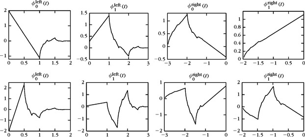
Theorem 7.17 constructs appropriate boundary scaling functions {ϕleftn}0≤n<p and {ϕrightn}0≤n<p.
Theorem 7.17:
Cohen, Daubechies, Vial. One can construct boundary scaling functions ϕleftn and ϕrightn so that if 2−j ≥ 2p, then ![]() is an orthonormal basis of a space Vjint satisfying
is an orthonormal basis of a space Vjint satisfying

and the restrictions to [0, 1] of polynomials of degree p − 1 are in Vjint.
Proof.
A sketch of the proof is given. All details are in [174]. Since the wavelet ψ corresponding to ϕ has p vanishing moments, the Fix-Strang condition (7.70) implies that
is a polynomial of degree k. At any scale 2j, qk(2−jt) is still a polynomial of degree k, and for 0 ≤ k < p this family defines a basis of polynomials of degree p − 1. To guarantee that polynomials of degree p − 1 are in Vjint we impose that the restriction of qk(2−jt) to [0, 1] can be decomposed in the basis of Vjint:
 (7.184)
Since the support of ϕ is [–p + 1, p], the condition (7.184) together with (7.183) can be separated into two nonoverlapping left and right conditions. With a change of variable, we verify that (7.184) is equivalent to
 (7.185)
 (7.186)
The embedding property Vjint⊂Vj − 1int is obtained by imposing that the boundary scaling functions satisfy scaling equations. We suppose that ϕleftn has a support [0, p + n] and satisfies a scaling equation of the form
 (7.187)
whereas φrightn has a support [–p –n, 0] and satisfies a similar scaling equation on the right. The constants Hleftn, l, hleftn, m, Hrightn, l, and hrightn, m are adjusted to verify the polynomial reproduction equations (7.185) and (7.186), while producing orthogonal scaling functions. The resulting family ![]() is an orthonormal basis of a space Vjint.
is an orthonormal basis of a space Vjint.
The convergence of the spaces Vjint to L2[0, 1] when 2j goes to 0 is a consequence of the fact that the multiresolution spaces Vj generated by the Daubechies scaling function {ϕj, n}n∈![]() converge to L2(
converge to L2(![]() ).
).
The proof constructs the scaling functions through scaling equations specified by discrete filters. At the boundaries, the filter coefficients are adjusted to construct orthogonal scaling functions with a support in [0, 1], and to guarantee that polynomials of degree p − 1 are reproduced by these scaling functions. Table 7.5 gives the filter coefficients for p = 2.

Wavelet Basis of L2[0, 1]
Let Wjint be the orthogonal complement of Vjint in Vj − 1int. The support of the Daubechies wavelet ψ with p vanishing moments is [–p + 1, p]. Since ϕj, n is orthogonal to any ϕj, l, we verify that an orthogonal basis of Wjint can be constructed with the 2−j − 2p inside wavelets with support in [0, 1]:
to which are added 2p left and right boundary wavelets
Since Wintj ⊂ Vintj–1 the left and right boundary wavelets at any scale 2j can be expanded into scaling functions at the scale 2j–1. For j=1 we impose that the left boundary wavelets satisfy equations of the form
 (7.188)
The right boundary wavelets satisfy similar equations. The coefficients Gleftn,l, gleftn,m, Grightn,l, and grightn,m are computed so that {ψintj,n}0 ≤n<2−j is an orthonormal basis of Wintj. Table 7.5 gives the values of these coefficients for p = 2.
For any 2J ≤ (2p)−1 the multiresolution properties prove that
is an orthonormal wavelet basis of L2[0, 1]. The boundary wavelets, like the inside wavelets, have p vanishing moments because polynomials of degree p − 1 are included in the space Vintj. Figure 7.18 displays the 2p = 4 boundary scaling functions and wavelets.
Fast Discrete Algorithm
For any f ∈ L2[0, 1] we denote
Wavelet coefficients are computed with a cascade of convolutions identical to Theorem 7.10 as long as filters do not overlap signal boundaries. A Daubechies filter h is considered here to have a support located at [– p + 1, p]. At the boundary, the usual Daubechies filters are replaced by boundary filters that relate boundary wavelets and scaling functions to the finer-scale scaling functions in (7.187) and (7.188).
Theorem 7.18:
Cohen, Daubechies, Vial. If 0 ≤ k < p,

This cascade algorithm decomposes aL into a discrete wavelet transform [aJ, {dj}L<j ≤J] with O(N) operations. The maximum scale must satisfy 2J ≤ (2p)−1, because the number of boundary coefficients remains equal to 2p at all scales. The implementation is more complicated than the folding and periodic algorithms described in Sections 7.5.1 and 7.5.2, but does not require more computations. The signal aL is reconstructed from its wavelet coefficients, by inverting the decomposition formula in Theorem 7.18.


7.6 MULTISCALE INTERPOLATIONS
Multiresolution approximations are closely connected to the generalized interpolations and sampling theorems studied in Section 3.1.3. Section 7.6.1 constructs general classes of interpolation functions from orthogonal scaling functions and derives new sampling theorems. Interpolation bases have the advantage of easily computing the decomposition coefficients from the sample values of the signal. Section 7.6.2 constructs interpolation wavelet bases.
7.6.1 Interpolation and Sampling Theorems
Section 3.1.3 explains that a sampling scheme approximates a signal by its orthogonal projection onto a space Us and samples this projection at intervals s. The space Us is constructed so that any function in Us can be recovered by interpolating a uniform sampling at intervals s. We relate the construction of interpolation functions to orthogonal scaling functions and compute the orthogonal projector on Us.
An interpolation function any ϕ such that {ϕ(t – n)}n ∈![]() is a Riesz basis of the space U1 it generates, and that satisfies
is a Riesz basis of the space U1 it generates, and that satisfies
Any f ∈ U1 is recovered by interpolating its samples f(n):
Indeed, we know that f is a linear combination of the basis vector {ϕ(t – n)}n ε![]() and the interpolation property (7.190) yields (7.191). The Whittaker sampling Theorem 3.2 is based on the interpolation function
and the interpolation property (7.190) yields (7.191). The Whittaker sampling Theorem 3.2 is based on the interpolation function
In this case, space U1 is the set of functions having a Fourier transform support included in [–π, π].
Scaling an interpolation function yields a new interpolation for a different sampling interval. Let us define ϕs(t) = ϕ(t/s) and
One can verify that any f ∈ Us can be written as
Scaling Autocorrelation
We denote by ϕo an orthogonal scaling function, defined by the fact that {ϕo (t – n)}n ε![]() is an orthonormal basis of a space V0 of a multiresolution approximation. Theorem 7.2 proves that this scaling function is characterized by a conjugate mirror filter ho. Theorem 7.20 defines an interpolation function from the autocorrelation of ϕo [423].
is an orthonormal basis of a space V0 of a multiresolution approximation. Theorem 7.2 proves that this scaling function is characterized by a conjugate mirror filter ho. Theorem 7.20 defines an interpolation function from the autocorrelation of ϕo [423].
Theorem 7.20.
is an interpolation function. Moreover,
Proof.
which proves the interpolation property (7.190). To prove that {ϕ(t – n)}n ∈![]() is a Riesz basis of the space U1 it generates, we verify the condition (7.9). The autocorrelation
is a Riesz basis of the space U1 it generates, we verify the condition (7.9). The autocorrelation ![]() has a Fourier transform
has a Fourier transform ![]() . Thus, condition (7.9) means that there exist B ≥ A > 0 such that
. Thus, condition (7.9) means that there exist B ≥ A > 0 such that
 (7.196)
We proved in (7.14) that the orthogonality of a family {ϕo(t – n)}n ∈![]() is equivalent to
is equivalent to
 (7.197)
Therefore, the right inequality of (7.196) is valid for A = 1. Let us prove the left inequality. Since ![]() one can verify that there exists K > 0 such that for all
one can verify that there exists K > 0 such that for all ![]() , so (7.197) implies that
, so (7.197) implies that ![]() It follows that
It follows that

which proves (7.196) for A−1 = 4(2K + 1).
Since ϕo is a scaling function, (7.23) proves that there exists a conjugate mirror filter ho such that
Computing ![]() yields (7.194) with
yields (7.194) with ![]()
Theorem 7.20 proves that the autocorrelation of an orthogonal scaling function ϕo is an interpolation function ϕ that also satisfies a scaling equation. One can design ϕ to approximate regular signals efficiently by their orthogonal projection in Us. Definition 6.1 measures the regularity of f with a Lipschitz exponent, which depends on the difference between f and its Taylor polynomial expansion. Theorem 7.21 gives a condition for recovering polynomials by interpolating their samples with ϕ. It derives an upper bound for the error when approximating f by its orthogonal projection in Us.
Theorem 7.21:
Fix, Strang. Any polynomial q(t) of degree smaller or equal to p − 1 is decomposed into
if and only if ![]() has a zero of order p at ω = π.
has a zero of order p at ω = π.
Suppose that this property is satisfied. If f has a compact support and is uniformly Lipschitz α ≤ p, then there exists C > 0 such that
Proof.
The main steps of the proof are given without technical detail. Let us set s = 2j. One can verify that the spaces {Vj = U2j}j ∈![]() define a multiresolution approximation of L2(
define a multiresolution approximation of L2(![]() ). The Riesz basis of V0 required by Definition 7.1 is obtained with θ = ϕ. This basis is orthogonalized by Theorem 7.1 to obtain an orthogonal basis of scaling functions. Theorem 7.3 derives a wavelet orthonormal basis {ψj,n}(j,n) ∈
). The Riesz basis of V0 required by Definition 7.1 is obtained with θ = ϕ. This basis is orthogonalized by Theorem 7.1 to obtain an orthogonal basis of scaling functions. Theorem 7.3 derives a wavelet orthonormal basis {ψj,n}(j,n) ∈![]() 2 of L2 (
2 of L2 (![]() ).
).
Using Theorem 7.4, one can verify that ψ has p vanishing moments if and only if ![]() has p zeros at π. Although ϕ is not the orthogonal scaling function, the Fix-Strang condition (7.70) remains valid. It is also equivalent that for k < p,
has p zeros at π. Although ϕ is not the orthogonal scaling function, the Fix-Strang condition (7.70) remains valid. It is also equivalent that for k < p,
is a polynomial of degree k. The interpolation property (7.191) implies that qk(n) = nk for all n ∈ ![]() , so qk(t) = tk. Since {tk}0⩽k<p is a basis for polynomials of degree p −1, any polynomial q(t) of degree p − 1 can be decomposed over {ϕ(t – n)}n ∈
, so qk(t) = tk. Since {tk}0⩽k<p is a basis for polynomials of degree p −1, any polynomial q(t) of degree p − 1 can be decomposed over {ϕ(t – n)}n ∈![]() if and only if
if and only if ![]() has p zeros at π.
has p zeros at π.
We indicate how to prove (7.199) for s = 2j. The truncated family of wavelets {ψl,n}l⩽j,n ∈![]() is an orthogonal basis of the orthogonal complement of U2j = Vj in L2(
is an orthogonal basis of the orthogonal complement of U2j = Vj in L2(![]() ). Thus,
). Thus,
If f is uniformly Lipschitz α, since ψ has p vanishing moments, Theorem 6.3 proves that there exists A > 0 such that
To simplify the argument we suppose that ψ has a compact support, although this is not required. Since f also has a compact support, one can verify that the number of nonzero 〈f, ψl,n〉 is bounded by K 2−l for some K > 0. Thus,

which proves (7.199) for s = 2j.
As long as α ≤ p, the larger the Lipschitz exponent α, the faster the error ‖ f – PUs f ‖ decays to zero when the sampling interval s decreases. If a signal f is Ck with a compact support, then it is uniformly Lipschitz k, so Theorem 7.21 proves that ‖ f – PUs f ‖ ≤ Csk.
EXAMPLE 7.11
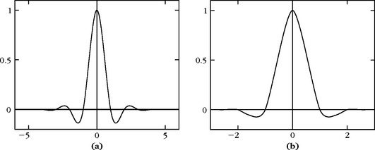
A cubic spline-interpolation function is obtained from the linear spline-scaling function ϕo. The Fourier transform expression (7.5) yields
Figure 7.19(a) gives the graph of ϕ, which has an infinite support but exponential decay. With Theorem 7.21, one can verify that this interpolation function recovers polynomials of degree 3 from a uniform sampling. The performance of spline interpolation functions for generalized sampling theorems is studied in [162, 468].
EXAMPLE 7.12
Deslauriers-Dubuc[206] interpolation functions of degree 2p − 1 are compactly supported interpolation functions of minimal size that decompose polynomials of degree 2p − 1. One can verify that such an interpolation function is the autocorrelation of a scaling function ϕo. To reproduce polynomials of degree 2p − 1, Theorem 7.21 proves that ![]() must have a zero of order 2p at π. Since
must have a zero of order 2p at π. Since ![]() it follows that
it follows that ![]() and thus
and thus ![]() has a zero of order p at π. The Daubechies theorem (7.7) designs minimum-size conjugate mirror filters ho that satisfy this condition. Daubechies filters ho have 2p nonzero coefficients and the resulting scaling function ϕo has a support of size 2p − 1. The autocorrelation ϕ is the Deslauriers-Dubuc interpolation function, which support [− 2p + 1, 2p − 1].
has a zero of order p at π. The Daubechies theorem (7.7) designs minimum-size conjugate mirror filters ho that satisfy this condition. Daubechies filters ho have 2p nonzero coefficients and the resulting scaling function ϕo has a support of size 2p − 1. The autocorrelation ϕ is the Deslauriers-Dubuc interpolation function, which support [− 2p + 1, 2p − 1].
For p = 1, ϕo = 1[0,1] and ϕ are the piecewise linear tent functions with a support that [– 1, 1]. For p = 2, the Deslauriers-Dubuc interpolation function ϕ is the autocorrelation of the Daubechies 2 scaling function, shown in Figure 7.10. The graph of this interpolation function is in Figure 7.19(b). Polynomials of degree 2p − 1 = 3 are interpolated by this function.
The scaling equation (7.194) implies that any autocorrelation filter verifies h[2n] =0 for n ≠ 0. For any p ≤0, the nonzero values of the resulting filter are calculated from the coefficients of the polynomial (7.168) that is factored to synthesize Daubechies filters. The support of h is[− 2p + 1, 2p − 1] and
Dual Basis
If f ∉ Us, then it is approximated by its orthogonal projection PUs f on Us before the samples at intervals s are recorded. This orthogonal projection is computed with a biorthogonal basis ![]() [82]. Theorem 3.4 proves that
[82]. Theorem 3.4 proves that ![]() where the Fourier transform of ϕ is
where the Fourier transform of ϕ is
 (7.202)
Figure 7.20 gives the graph of the cubic spline ![]() associated to the cubic spline-interpolation function. The orthogonal projection of f over Us is computed by decomposing f in the biorthogonal bases
associated to the cubic spline-interpolation function. The orthogonal projection of f over Us is computed by decomposing f in the biorthogonal bases
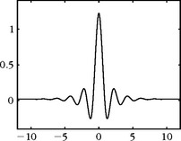
FIGURE 7.20 The dual cubic spline ![]() (t) associated to the cubic spline-interpolation function ϕ(t) shown in Figure 7.19(a).
(t) associated to the cubic spline-interpolation function ϕ(t) shown in Figure 7.19(a).
Let ![]() The interpolation property (7.190) implies that
The interpolation property (7.190) implies that
Therefore, this discretization of f through a projection onto Us is obtained by a filtering with ![]() followed by a uniform sampling at intervals s. The best linear approximation of f is recovered with the interpolation formula (7.203).
followed by a uniform sampling at intervals s. The best linear approximation of f is recovered with the interpolation formula (7.203).
7.6.2 Interpolation Wavelet Basis
An interpolation function ϕ can recover a signal f from a uniform sampling {f(ns)}n ∈![]() if f belongs to an appropriate subspace Us of L2(
if f belongs to an appropriate subspace Us of L2(![]() ). Donoho [213] has extended this approach by constructing interpolation wavelet bases of the whole space of uniformly continuous signals with the supremum norm. The decomposition coefficients are calculated from sample values instead of inner product integrals.
). Donoho [213] has extended this approach by constructing interpolation wavelet bases of the whole space of uniformly continuous signals with the supremum norm. The decomposition coefficients are calculated from sample values instead of inner product integrals.
Subdivision Scheme
Let ϕ be an interpolation function that is the autocorrelation of an orthogonal scaling function ϕo. Let ϕj,n(t) = ϕ(2−j t – n). The constant 2−j/2 that normalizes the energy of ϕj,n is not added because we shall use a supremum norm ‖ f ‖∞ = supt ε![]() |f (t)| instead of the L2 (
|f (t)| instead of the L2 (![]() ) norm, and
) norm, and
We define the interpolation space Vj of functions
where a[n] has at most a polynomial growth in n. Since ϕ is an interpolation function, a [n] =g(2j n). This space Vj is not included in L2(![]() ) since a[n] may not have a finite energy. The scaling equation (7.194) implies that Vj+1 ⊂ Vj for any j ∈
) since a[n] may not have a finite energy. The scaling equation (7.194) implies that Vj+1 ⊂ Vj for any j ∈![]() . If the autocorrelation filter h has a Fourier transform
. If the autocorrelation filter h has a Fourier transform ![]() that has a zero of order p at ω = π, then Theorem 7.21 proves that polynomials of a degree smaller than p − 1 are included in Vj.
that has a zero of order p at ω = π, then Theorem 7.21 proves that polynomials of a degree smaller than p − 1 are included in Vj.
For f ∉ Vj, we define a simple projector on Vj that interpolates the dyadic samples f (2j n):
This projector has no orthogonality property but satisfies PVj f (2j n) = f (2j n). Let C0 be the space of functions that are uniformly continuous over ![]() . Theorem 7.22 proves that any f ε C0 can be approximated with an arbitrary precision by PVj f when 2j goes to zero.
. Theorem 7.22 proves that any f ε C0 can be approximated with an arbitrary precision by PVj f when 2j goes to zero.
Theorem 7.22:
Donoho. Suppose that ϕ has an exponential decay. If f ∈ C0, then
Proof. Let ω(δ, f) denote the modulus of continuity
Any t ε ![]() can be written as t = 2j(n + h) with n ε
can be written as t = 2j(n + h) with n ε ![]() and |h| ≤ 1. Since PVj f (2jn) = f (2jn),
and |h| ≤ 1. Since PVj f (2jn) = f (2jn),

Lemma 7.3 proves that ω(2j, PVj f) ≤ Cϕ ω(2j, f) where Cϕ is a constant independent of j and f. Taking a supremum over t = 2j(n + h) implies the final result:
Lemma 7.3.
There exists Cϕ > 0 such that for all j ε ![]() and f ε C0,
and f ε C0,
Let us set j = 0. For |h| ≤ 1, a summation by parts gives
Since ϕ has an exponential decay, there exists a constant Cϕ such that if |h| ≤ 1 and t ε ![]() , then
, then ![]() . Taking a supremum over t in (7.209) proves that
. Taking a supremum over t in (7.209) proves that
Scaling this result by 2j yields (7.208).
Interpolation Wavelets
The projection PVj f (t) interpolates the values f (2j n). When reducing the scale by 2, we obtain a finer interpolation PVj–1 f (t) that also goes through the intermediate samples f (2j(n + 1/2)). This refinement can be obtained by adding “details” that compensate for the difference between PVjf (2j(n + 1/2)) and f (2j (n + 1/2)). To do this, we create a “detail” space Wj that provides the values f (t) at intermediate dyadic points t = 2j (n + 1/2). This space is constructed from interpolation functions centered at these locations, namely ϕj–1,2n+1. We call interpolation wavelets
Observe that ψj,n(t) = ψ(2−j t – n) with
The function ψ is not truly a wavelet since it has no vanishing moment. However, we shall see that it plays the same role as a wavelet in this decomposition. We define Wj to be the space of all sums ![]() . Theorem 7.23 proves that it is a (nonorthogonal) complement of Vj in Vj–1.
. Theorem 7.23 proves that it is a (nonorthogonal) complement of Vj in Vj–1.
Proof.
Any f ε Vj–1 can be written as
The function f – PVj f belongs to Vj–1 and vanishes at {2j n}n ε![]() . Thus, it can be decomposed over the intermediate interpolation functions ϕj–1,2n+1 = ψj, n:
. Thus, it can be decomposed over the intermediate interpolation functions ϕj–1,2n+1 = ψj, n:
This proves that Vj–1 ⊂ Vj ⊕ Wj. By construction we know that Wj ⊂ Vj–1, so Vj–1 =Vj ⊕ Wj. Setting t = 2j–1(2n + 1) in this formula also verifies (7.210).
Theorem 7.23 refines an interpolation from a coarse grid 2j n to a finer grid 2j–1 n by adding “details” with coefficients dj[n] that are the interpolation errors f (2j(n + 1/2)) – PVj f (2j(n + 1/2)). The following Theorem 7.24 defines an interpolation wavelet basis of C0 in the sense of uniform convergence.
Theorem 7.24.
 (7.211)
The formula (7.211) decomposes f into a coarse interpolation at intervals 2J plus layers of details that give the interpolation errors on successively finer dyadic grids. The proof is done by choosing f to be a continuous function with a compact support, in which case (7.211) is derived from Theorem 7.23 and (7.206). The density of such functions in C0 (for the supremum norm) allows us to extend this result to any f in C0. We shall write

which means that [{ϕJ,n}n ε![]() , {ψj,n}n ε
, {ψj,n}n ε![]() , j≤J] is abasis of C0. In L2 (
, j≤J] is abasis of C0. In L2 (![]() ), “biorthogonal” scaling functions and wavelets are formally defined by
), “biorthogonal” scaling functions and wavelets are formally defined by
Clearly, ![]() Similarly, (7.210) and (7.205) implies that
Similarly, (7.210) and (7.205) implies that ![]() is a finite sum of Diracs. These dual-scaling functions and wavelets do not have a finite energy, which illustrates the fact that
is a finite sum of Diracs. These dual-scaling functions and wavelets do not have a finite energy, which illustrates the fact that ![]() is not a Riesz basis of L2 (
is not a Riesz basis of L2 (![]() ).
).
If ![]() has p zeros at π, then one can verify that
has p zeros at π, then one can verify that ![]() has p vanishing moments. With similar derivations as in the proof of (6.20) in Theorem 6.4, one can show that if f is uniformly Lipschitz α ≤ p, then there exists A > 0 such that
has p vanishing moments. With similar derivations as in the proof of (6.20) in Theorem 6.4, one can show that if f is uniformly Lipschitz α ≤ p, then there exists A > 0 such that
A regular signal yields small-amplitude wavelet coefficients at fine scales. Thus, we can neglect these coefficients and still reconstruct a precise approximation of f.
Fast Calculations
The interpolating wavelet transform of f is calculated at scale 1 ≥ 2j > N−1 = 2L from its sample values {f(N−1n)}n ε![]() . At each scale 2j, the values of f in between samples {2j n}n ε
. At each scale 2j, the values of f in between samples {2j n}n ε![]() are calculated with the interpolation (7.205):
are calculated with the interpolation (7.205):
 (7.213)
where the interpolation filter hi is a subsampling of the autocorrelation filter h in (7.195):
The wavelet coefficients are computed with (7.210):
The reconstruction of f (N−1 n) from the wavelet coefficients is performed recursively by recovering the samples f (2j–1 n) from the coarser sampling f (2j n) with the interpolation (7.213) to which is added dj[n]. If hi[n] is a finite filter of size K and if f has a support in [0, 1], then the decomposition and reconstruction algorithms require KN multiplications and additions.
A Deslauriers-Dubuc interpolation function ϕ has the shortest support while including polynomials of degree 2p − 1 in the spaces Vj. The corresponding interpolation filter hi[n] defined by (7.214) has 2p nonzero coefficients for –p ≤n < p, which are calculated in (7.201). If p = 2, then hi[1] = hi[–2] = −1/16 and hi[0] = hi[– 1] = 9/16. Suppose that q(t) is apolynomial of degree smaller or equal to 2p − 1. Since q = PVjq, (7.213) implies a Lagrange interpolation formula
The Lagrange filter hi of size 2p is the shortest filter that recovers intermediate values of polynomials of degree 2p − 1 from a uniform sampling.
To restrict the wavelet interpolation bases to a finite interval [0, 1] while reproducing polynomials of degree 2p − 1, the filter hi is modified at the boundaries. Suppose that f (N−1 n) is defined for 0 ≤ n < N. When computing the interpolation

if n is too close to 0 or to 2−j − 1, then hi must be modified to ensure that the support of hi [n – k] remains inside [0, 2−j − 1]. The interpolation PVjf (2j (n + 1/2)) is then calculated from the closest 2p samples f (2j k) for 2j k ε [0, 1]. The new interpolation coefficients are computed in order to recover exactly all polynomials of degree 2p − 1 [450]. For p = 2, the problem occurs only at n = 0 and the appropriate boundary coefficients are
The symmetric boundary filter hi[–n] is used on the other side at n = 2−j − 1.
7.7 SEPARABLE WAVELET BASES
To any wavelet orthonormal basis {ψj,n}(j,n) ε![]() 2 of L2(
2 of L2(![]() ), one can associate a separable wavelet orthonormal basis of L2(
), one can associate a separable wavelet orthonormal basis of L2(![]() 2):
2):
The functions ψj1,n1 (x1) ψj2,n2(x2) mix information at two different scales 2j1 and 2j2 along x1 and x2, which we often want to avoid. Separable multiresolutions lead to another construction of separable wavelet bases with wavelets that are products of functions dilated at the same scale. These multiresolution approximations also have important applications in computer vision, where they are used to process images at different levels of details. Lower-resolution images are indeed represented by fewer pixels and might still carry enough information to perform a recognition task.
Signal decompositions in separable wavelet bases are computed with a separable extension of the filter bank algorithm described in Section 7.7.3. Section 7.7.4 constructs separable wavelet bases in any dimension, and explains the corresponding fast wavelet transform algorithm. Nonseparable wavelet bases can also be constructed [85, 334] but they are used less often in image processing. Section 7.8.3 gives examples of nonseparable quincunx biorthogonal wavelet bases, which have a single quasi-istropic wavelet at each scale.
7.7.1 Separable Multiresolutions
As in one dimension, the notion of resolution is formalized with orthogonal projections in spaces of various sizes. The approximation of an image f(x1, x2) at the resolution 2−j is defined as the orthogonal projection of f on a space V2j that is included in L2(![]() 2). The space V2j is the set of all approximations at the resolution 2−j. When the resolution decreases, the size of V2j decreases as well. The formal definition of a multiresolution approximation {V2j}j ε
2). The space V2j is the set of all approximations at the resolution 2−j. When the resolution decreases, the size of V2j decreases as well. The formal definition of a multiresolution approximation {V2j}j ε![]() of L2(
of L2(![]() 2) is a straightforward extension of Definition 7.1 that specifies multiresolutions of L2(
2) is a straightforward extension of Definition 7.1 that specifies multiresolutions of L2(![]() ). The same causality, completeness, and scaling properties must be satisfied.
). The same causality, completeness, and scaling properties must be satisfied.
We consider the particular case of separable multiresolutions. Let {Vj}j ε![]() be a multiresolution of L2(
be a multiresolution of L2(![]() ). A separable two-dimensional multiresolution is composed of the tensor product spaces
). A separable two-dimensional multiresolution is composed of the tensor product spaces
The space V2j is the set of finite energy functions f (x1, x2) that are linear expansions of separable functions:
Section A.5 reviews the properties of tensor products. If {Vj}j ε![]() is a multiresolution approximation of L2(
is a multiresolution approximation of L2(![]() ), then {V2j}j ε
), then {V2j}j ε![]() is a multiresolution approximation of L2(
is a multiresolution approximation of L2(![]() 2).
2).
Theorem 7.1 demonstrates the existence of a scaling function ϕ such that {ϕj,m}m ε![]() is an orthonormal basis of Vj. Since Vj2j = Vj ⊗ Vj, Theorem A.6 proves that for x = (x1, x2) and n = (n1, n2),
is an orthonormal basis of Vj. Since Vj2j = Vj ⊗ Vj, Theorem A.6 proves that for x = (x1, x2) and n = (n1, n2),
is an orthonormal basis of V2j. It is obtained by scaling by 2j the two-dimensional separable scaling function ϕ2(x) = ϕ(x1) ϕ(x2) and translating it on a two-dimensional square grid with intervals 2j.
EXAMPLE 7.13 Piecewise Constant Approximation
Let Vj be the approximation space of functions that are constant on [2jm, 2j(m + 1)] for any m ∈ ![]() . The tensor product defines a two-dimensional piecewise constant approximation. The space V2j is the set of functions that are constant on any square [2j n1, 2j(n1 + 1)] × [2j n2, 2j(n2 + 1)], for (n1, n2) ε
. The tensor product defines a two-dimensional piecewise constant approximation. The space V2j is the set of functions that are constant on any square [2j n1, 2j(n1 + 1)] × [2j n2, 2j(n2 + 1)], for (n1, n2) ε ![]() 2. The two-dimensional scaling function is
2. The two-dimensional scaling function is
EXAMPLE 7.14 Shannon Approximation
Let Vj be the space of functions with Fourier transforms that have a support included in [–2−j π, 2−j π]. Space V2j is the set of functions the two-dimensional Fourier transforms of which have a support included in the low-frequency square [–2−j π, 2−j π] ×[–2−j, 2−j π]. The two-dimensional scaling function is a perfect two-dimensional low-pass filter the Fourier transform of which is
EXAMPLE 7.15 Spline Approximation
Let Vj be the space of polynomial spline functions of degree p that are Cp–1 with nodes located at 2−jm for m ε ![]() . The space V2j is composed of two-dimensional polynomial spline functions that are p − 1 times continuously differentiable. The restriction of f (x1, x2) ε V2j to any square [2jn1, 2j (n1 + 1)] × [2j n2, 2j(n2 + 1)] is a separable product q1(x1)q2(x2) of two polynomials of degree at most p.
. The space V2j is composed of two-dimensional polynomial spline functions that are p − 1 times continuously differentiable. The restriction of f (x1, x2) ε V2j to any square [2jn1, 2j (n1 + 1)] × [2j n2, 2j(n2 + 1)] is a separable product q1(x1)q2(x2) of two polynomials of degree at most p.
Multiresolution Vision
An image of 512 × 512 pixels often includes too much information for real-time vision processing. Multiresolution algorithms process less image data by selecting the relevant details that are necessary to perform a particular recognition task [58]. The human visual system uses a similar strategy. The distribution of photoreceptors on the retina is not uniform. The visual acuity is greatest at the center of the retina where the density of receptors is maximum. When moving apart from the center, the resolution decreases proportionally to the distance from the retina center [428].
The high-resolution visual center is called the fovea. It is responsible for high-acuity tasks such as reading or recognition. A retina with a uniform resolution equal to the highest fovea resolution would require about 10,000 times more photoreceptors. Such a uniform resolution retina would increase considerably the size of the optic nerve that transmits the retina information to the visual cortex and the size of the visual cortex that processes these data.
Active vision strategies [83] compensate the nonuniformity of visual resolution with eye saccades, which move successively the fovea over regions of a scene with a high information content. These saccades are partly guided by the lower-resolution information gathered at the periphery of the retina. This multiresolution sensor has the advantage of providing high-resolution information at selected locations and a large field of view with relatively little data.
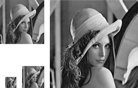
Multiresolution algorithms implement in software [125] the search for important high-resolution data. A uniform high-resolution image is measured by a camera but only a small part of this information is processed. Figure 7.21 displays a pyramid of progressively lower-resolution images calculated with a filter bank presented in Section 7.7.3. Coarse to fine algorithms analyze first the lower-resolution image and selectively increase the resolution in regions where more details are needed. Such algorithms have been developed for object recognition and stereo calculations [284].
7.7.2 Two-Dimensional Wavelet Bases
A separable wavelet orthonormal basis of L2 (![]() 2) is constructed with separable products of a scaling function ϕ and a wavelet ψ. The scaling function ϕ is associated to a one-dimensional multiresolution approximation {Vj}j ε
2) is constructed with separable products of a scaling function ϕ and a wavelet ψ. The scaling function ϕ is associated to a one-dimensional multiresolution approximation {Vj}j ε![]() Let {V2j}j ε
Let {V2j}j ε![]() be the separable two-dimensional multiresolution defined by V2j = Vj ⊗ Vj. Let W2j be the detail space equal to the orthogonal complement of the lower-resolution approximation space V2j in V2j–1:
be the separable two-dimensional multiresolution defined by V2j = Vj ⊗ Vj. Let W2j be the detail space equal to the orthogonal complement of the lower-resolution approximation space V2j in V2j–1:
To construct a wavelet orthonormal basis of L2(![]() 2), Theorem 7.25 builds a wavelet basis of each detail space W2j
2), Theorem 7.25 builds a wavelet basis of each detail space W2j
Theorem 7.25.
Let ϕ be a scaling function and ψ be the corresponding wavelet generating a wavelet orthonormal basis of L2(![]() ). We define three wavelets:
). We define three wavelets:
is an orthonormal basis of W2j, and
Proof.
Equation (7.217) is rewritten as
The one-dimensional multiresolution space Vj–1 can also be decomposed into Vj–1 =Vj ⊕ Wj. By inserting this in (7.221), the distributivity of ⊕ with respect to ⊗ proves that
Since {ϕj,m}m ε![]() and {ψj,m}m ε
and {ψj,m}m ε![]() are orthonormal bases of Vj and Wj, we derive that
are orthonormal bases of Vj and Wj, we derive that
is an orthonormal basis of W2j. As in the one-dimensional case, the overall space L2 (![]() 2) can be decomposed as an orthogonal sum of the detail spaces at all resolutions:
2) can be decomposed as an orthogonal sum of the detail spaces at all resolutions:
is an orthonormal basis of L2 (![]() 2).
2).
The three wavelets extract image details at different scales and in different directions. Overpositive frequencies, ![]() and
and ![]() have an energy mainly concentrated, respectively, on [0, π] and [π, 2π]. The separable wavelet expressions (7.218) imply that
have an energy mainly concentrated, respectively, on [0, π] and [π, 2π]. The separable wavelet expressions (7.218) imply that
and ![]() Thus,
Thus, ![]() is large at low horizontal frequencies ω1 and high vertical frequencies ω2, whereas
is large at low horizontal frequencies ω1 and high vertical frequencies ω2, whereas ![]() is large at high horizontal frequencies and low vertical frequencies, and
is large at high horizontal frequencies and low vertical frequencies, and ![]() is large at high horizontal and vertical frequencies. Figure 7.22 displays the Fourier transform of separable wavelets and scaling functions calculated from a one-dimensional Daubechies 4 wavelet.
is large at high horizontal and vertical frequencies. Figure 7.22 displays the Fourier transform of separable wavelets and scaling functions calculated from a one-dimensional Daubechies 4 wavelet.

FIGURE 7.22 Fourier transforms of a separable scaling function and of three separable wavelets calculated from a one-dimensional Daubechies 4 wavelet.
Suppose that ψ(t) has p vanishing moments and is orthogonal to one-dimensional polynomials of degree p − 1. The wavelet ψ1 has p one-dimensional directional vanishing moments along x2 in the sense that it is orthogonal to any function f(x1, x2) that is a polynomial of degree p − 1 along x2 for x1 fixed. It is a horizontal directional wavelet that yields large coefficients for horizontal edges, as explained in Section 5.5.1. Similarly, ψ2 has p − 1 directional vanishing moments along x1 and is a vertical directional wavelet. This is illustrated by the decomposition of a square later in Figure 7.24. The wavelet ψ3 has directional vanishing moments along both x1 and x2 and is therefore not a directional wavelet. It produces large coefficients at corners or junctions. The three wavelets ψk for k = 1, 2, 3 are orthogonal to two-dimensional polynomials of degree p − 1.

FIGURE 7.24 Separable wavelet transforms of the Lena image and of a white square in a black background, decomposed on 3 and 4 octaves, respectively. Black, gray, and white pixels correspond, respectively, to positive, zero, and negative wavelet coefficients. The disposition of wavelet image coefficients dkj[n, m] = 〈 f, ψkj,n 〉 is illustrated on the top left.
EXAMPLE 7.16
For a Shannon multiresolution approximation, the resulting two-dimensional wavelet basis paves the two-dimensional Fourier plane (ω1, ω2) with dilated rectangles. The Fourier transforms ![]() are the indicator functions of [–π, π] and [–2π, – π] ∪ [π, 2π], respectively. The separable space V2j contains functions with a two-dimensional Fourier transform support included in the low-frequency square [–2−j π, 2−j π] × [–2−j π, 2−j π]. This corresponds to the support of
are the indicator functions of [–π, π] and [–2π, – π] ∪ [π, 2π], respectively. The separable space V2j contains functions with a two-dimensional Fourier transform support included in the low-frequency square [–2−j π, 2−j π] × [–2−j π, 2−j π]. This corresponds to the support of ![]() indicated in Figure 7.23.
indicated in Figure 7.23.

FIGURE 7.23 These dyadic rectangles indicate the regions where the energy of ![]() is mostly concentrated for 1 ≤ k ≤ 3. Image approximations at the scale 2j are restricted to the lower-frequency square.
is mostly concentrated for 1 ≤ k ≤ 3. Image approximations at the scale 2j are restricted to the lower-frequency square.
The detail space W2j is the orthogonal complement of V2j in V2j–1 and thus includes functions with Fourier transforms supported in the frequency annulus between the two squares [−2−jπ, 2−jπ] × [–2−jπ, 2−jπ] and [–2−j+1π, 2−j+1π] × [−2−j+1π, 2−j+1π]. As shown in Figure 7.23, this annulus is decomposed in three separable frequency regions, which are the Fourier supports of ![]() for 1 ≤ k ≤ 3. Dilating these supports at all scales 2j yields an exact cover of the frequency plane (ω1, ω2).
for 1 ≤ k ≤ 3. Dilating these supports at all scales 2j yields an exact cover of the frequency plane (ω1, ω2).
For general separable wavelet bases, Figure 7.23 gives only an indication of the domains where the energy of the different wavelets is concentrated. When the wavelets are constructed with a one-dimensional wavelet of compact support, the resulting Fourier transforms have side lobes that appear in Figure 7.22.
EXAMPLE 7.17
Figure 7.24 gives two examples of wavelet transforms computed using separable Daubechies wavelets with p = 4 vanishing moments. They are calculated with the filter bank algorithm from Section 7.7.3. Coefficients of large amplitude in d1j, d2j, and d3j correspond, respectively, to vertical high frequencies (horizontal edges), horizontal high frequencies (vertical edges), and high frequencies in both directions (corners). Regions where the image intensity varies smoothly yield nearly zero coefficients, shown in gray in the figure. The large number of nearly zero coefficients makes it particularly attractive for compact image coding.
Separable Biorthogonal Bases
One-dimensional biorthogonal wavelet bases are extended to separable biorthogonal bases of L2 (![]() 2) with the same approach as in Theorem 7.25. Let ϕ, ψ and
2) with the same approach as in Theorem 7.25. Let ϕ, ψ and ![]() be two dual pairs of scaling functions and wavelets that generate biorthogonal wavelet bases of L2 (
be two dual pairs of scaling functions and wavelets that generate biorthogonal wavelet bases of L2 (![]() ). The dual wavelets of ψ1, ψ2, and ψ3 defined by (7.218) are
). The dual wavelets of ψ1, ψ2, and ψ3 defined by (7.218) are
7.7.3 Fast Two-Dimensional Wavelet Transform
The fast wavelet transform algorithm presented in Section 7.3.1 is extended in two dimensions. At all scales 2j and for any n = (n1, n2), we denote
For any pair of one-dimensional filters y[m] and z[m] we write the product filter yz[n] = y[n1]z[n2] and ![]() . Let h[m] and g[m] be the conjugate mirror filters associated to the wavelet ψ.
. Let h[m] and g[m] be the conjugate mirror filters associated to the wavelet ψ.
The wavelet coefficients at the scale 2j+1 are calculated from aj with two-dimensional separable convolutions and subsamplings. The decomposition formulas are obtained by applying the one-dimensional convolution formulas (7.102) and (7.103) of Theorem 7.10 to the separable two-dimensional wavelets and scaling functions for n = (n1, n2):
We showed in (3.70) that a separable two-dimensional convolution can be factored into one-dimensional convolutions along the rows and columns of the image. With the factorization illustrated in Figure 7.25(a), these four convolutions equations are computed with only six groups of one-dimensional convolutions. The rows of aj are first convolved with and ![]() and
and ![]() subsampled by 2. The columns of these two output images are then convolved, respectively with
subsampled by 2. The columns of these two output images are then convolved, respectively with ![]() and
and ![]() and subsampled, which gives the four subsampled images aj+1, d1j+1, d2j+1, and d3j+1.
and subsampled, which gives the four subsampled images aj+1, d1j+1, d2j+1, and d3j+1.

FIGURE 7.25 (a) Decomposition of aj with six groups of one-dimensional convolutions and subsamplings along the image rows and columns. (b) Reconstruction of aj by inserting zeros between the rows and columns of aj+1 and dkj+1, and filtering the output.
We denote by ![]() the image twice the size of y[n], obtained by inserting a row of zeros and a column of zeros between pairs of consecutive rows and columns. The approximation aj is recovered from the coarser-scale approximation aj+1 and the wavelet coefficients dkj+1 with two-dimensional separable convolutions derived from the one-dimensional reconstruction formula (7.104)
the image twice the size of y[n], obtained by inserting a row of zeros and a column of zeros between pairs of consecutive rows and columns. The approximation aj is recovered from the coarser-scale approximation aj+1 and the wavelet coefficients dkj+1 with two-dimensional separable convolutions derived from the one-dimensional reconstruction formula (7.104)
These four separable convolutions can also be factored into six groups of one-dimensional convolutions along rows and columns, illustrated in Figure 7.25(b).
Let b[n] be an input image with pixels at a distance 2L. We associate to b[n] a function f(x) ε V2L approximated at the scale 2L. Its coefficients aL [n] = 〈f, ϕ2L,n 〉 are defined like in (7.111) by
The wavelet image representation of aL is computed by iterating (7.227-7.230) for
The image aL is recovered from this wavelet representation by computing (7.231) for J > j ≥ L.
Finite Image and Complexity
When aL is a finite image of N =N1 N2 pixels, we face boundary problems when computing the convolutions (7.227-7.231). Since the decomposition algorithm is separable along rows and columns, we use one of the three one-dimensional boundary techniques described in Section 7.5. The resulting values are decomposition coefficients in a wavelet basis of L2[0, 1]2. Depending on the boundary treatment, this wavelet basis is a periodic basis, a folded basis, or a boundary adapted basis.
For square images with N1 = N2, the resulting images aj and dkj have 2−2j samples. Thus, the images of the wavelet representation (7.233) include a total of N samples. If h and g have size K, the reader can verify that 2K2−2(j–1) multiplications and additions are needed to compute the four convolutions (7.227-7.230) with the factorization of Figure 7.25(a). Thus, the wavelet representation (7.233) is calculated with fewer than 8/3 KN operations. The reconstruction of aL by factoring the reconstruction equation (7.231) requires the same number of operations.
Fast Biorthogonal Wavelet Transform
The decomposition of an image in a biorthogonal wavelet basis is performed with the same fast wavelet transform algorithm. Let (![]() ,
, ![]() ) be the perfect reconstruction filters associated to (h, g). The inverse wavelet transform is computed by replacing the filters (h, g) that appear in (7.231) by (
) be the perfect reconstruction filters associated to (h, g). The inverse wavelet transform is computed by replacing the filters (h, g) that appear in (7.231) by (![]() ,
, ![]() ).
).
7.7.4 Wavelet Bases in Higher Dimensions
Separable wavelet orthonormal bases of L2 (![]() p) are constructed for any p ≥ 2 with a procedure similar to the two-dimensional extension. Let ϕ be a scaling function and ψ a wavelet that yields an orthogonal basis of L2(
p) are constructed for any p ≥ 2 with a procedure similar to the two-dimensional extension. Let ϕ be a scaling function and ψ a wavelet that yields an orthogonal basis of L2(![]() ). We denote θ0 = ϕ and θ1 = ψ. To any integer 0 ≤ ε < 2p written in binary form ε = ε1, …, εp, we associate the p-dimensional functions defined in x = (x1, …, xp) by
). We denote θ0 = ϕ and θ1 = ψ. To any integer 0 ≤ ε < 2p written in binary form ε = ε1, …, εp, we associate the p-dimensional functions defined in x = (x1, …, xp) by
For ε = 0, we obtain a p-dimensional scaling function
Nonzero indexes ε correspond to 2p − 1 wavelets. At any scale 2j and for n =(n1, …, np), we denote
Theorem 7.26.
The family obtained by dilating and translating the 2p − 1 wavelets for ε ≠ 0,
is an orthonormal basis of L2(![]() p).
p).
The proof is done by induction on p. It follows the same steps as the proof of Theorem 7.25, which associates to a wavelet basis of L2(![]() ) a separable wavelet basis of L2(
) a separable wavelet basis of L2(![]() 2). For p = 2, we verify that the basis (7.234) includes three elementary wavelets. For p = 3, there are seven different wavelets.
2). For p = 2, we verify that the basis (7.234) includes three elementary wavelets. For p = 3, there are seven different wavelets.
Fast Wavelet Transform
Let b[n] be an input p-dimensional discrete signal sampled at intervals 2L. We associate b[n] to an approximation f at the scale 2L with scaling coefficients aL [n] = 〈f, ψ0L,n〉 that satisfy
The wavelet coefficients of f at scales 2j > 2L are computed with separable convolutions and subsamplings along the p signal dimensions. We denote
The fast wavelet transform is computed with filters that are separable products of the one-dimensional filters h and g. The separable p-dimensional low-pass filter is
Let us denote u0 [m] = h[m] and u1 [m] =g[m]. To any integer ε = ε1,…, εp written in a binary form, we associate a separable p-dimensional band-pass filter
We denote by ![]() the signal obtained by adding a zero between any two samples of y[n] that are adjacent in the p-dimensional lattice n= (n1, …, np). It doubles the size of y[n] along each direction. If y[n] has Mp samples, then y[n] has (2M)p samples. The reconstruction is performed with
the signal obtained by adding a zero between any two samples of y[n] that are adjacent in the p-dimensional lattice n= (n1, …, np). It doubles the size of y[n] along each direction. If y[n] has Mp samples, then y[n] has (2M)p samples. The reconstruction is performed with
 (7.237)
The 2p separable convolutions needed to compute aj and {dεj}1≤ε ≤2p as well as the reconstruction (7.237) can be factored in 2p+1 − 2 groups of one-dimensional convolutions along the rows of p-dimensional signals. This is a generalization of the two-dimensional case, illustrated in Figure 7.25. The wavelet representation of aL is
It is computed by iterating (7.235) and (7.236) for L ≤ j < J. The reconstruction of aL is performed with the partial reconstruction (7.237) for J >j ≥ L.
If aL is a finite signal of size N1, …, Np, the one-dimensional convolutions are modified with one of the three boundary techniques described in Section 7.5. The resulting algorithm computes decomposition coefficients in a separable wavelet basis of L2[0, 1]p. If N1 = … = Np, the signals aj and dεj have 2−pj samples. Like aL, the wavelet representation (7.238) is composed of N samples. If the filter h has K nonzero samples, then the separable factorization of (7.235) and (7.236) requires pK2−p(j–1) multiplications and additions. Thus, the wavelet representation (7.238) is computed with fewer than p (1 − 2−p) −1KN multiplications and additions. The reconstruction is performed with the same number of operations.
7.8 LIFTING WAVELETS
The lifting scheme, introduced by Sweldens [451, 452], factorizes orthogonal and biorthogonal wavelet transforms into elementary spatial operators called liftings. It has two main applications. The first one is an acceleration of the fast wavelet transform algorithm. The filter bank convolution and subsampling operations are factorized into elementary filterings on even and odd samples, which reduces the number of operations by nearly 2. Border treatments are also simplified. This is also called a paraunitary filter bank implementation. Readers mainly interested in this fast lifting implementation can skip directly to Section 7.8.5, which can be read independently.
The second application is the design of wavelets adapted to multidimensional-bounded domains and surfaces, which is not possible with a Fourier transform approach. Section 7.8.1 introduces biorthogonal multiresolution and wavelet bases over nonstationary grids for arbitrary domains. The lifting construction of biorthogonal wavelet bases is explained in Section 7.8.2, with the resulting fast lifting wavelet transform. Section 7.8.3 describes an application to nonseparable quincunx wavelet bases for images. The construction of wavelet bases over bounded domains and surfaces is explained in Section 7.8.4, with computer graphics examples.
7.8.1 Biorthogonal Bases over Nonstationary Grids
The lifting scheme constructs wavelet bases over an arbitrary domain Ω to represent functions of finite energy defined over Ω. This section defines biorthogonal filters and wavelets that may be modified both in space and in scale to be adapted to the domain geometry. Section 7.8.2 explains the calculation of these filters and wavelets with a lifting scheme.
Embedded Grids
Biorthogonal multiresolutions, defined in Section 7.4, are generalized by considering nested spaces
which are defined over embedded approximation grids Gj ⊂ GJ–1. Each index n ε Gj is associated to a sampling point xn ε Ω. Since the sampling grids are embedded, this position does not change when the index is moved to finer grids n ε Gk for k ≤ j. Each space Vj is equipped with a Riesz basis {ϕj,n}n εGj parameterized by the approximation grid Gj.
Embedded grids are decomposed with complementary grids Cj:
For example, over the interval [0, 1], the grid Gj–1 is the set of 2j–1 n ∈ [0, 1] for 0 ≤ n < 2−j. It is decomposed into the even grid points of 2j–1 2n of Gj and the odd grid points 2j–1(2n + 1) of Cj. A corresponding vector space decomposition is defined Vj–1 = Vj ⊕ Wj, where the detail space Wj has a Riesz basis of wavelets {ψj,m}m εCj indexed on the complementary grid Cj.
A dual-biorthogonal wavelet family ![]() and a dual basis of scaling functions
and a dual basis of scaling functions ![]() satisfy the biorthogonality conditions
satisfy the biorthogonality conditions
The resulting wavelet families {ψj,m}m εGj,j ε![]() and
and ![]() are biorthogonal wavelet bases of L2(Ω), which implies that for any f ε L2(Ω),
are biorthogonal wavelet bases of L2(Ω), which implies that for any f ε L2(Ω),
where 2J is an arbitrary coarsest scale. The difference with the biorthogonal wavelets of Section 7.4 is that scaling functions and wavelets are typically not translations and dilations of mother scaling functions and wavelets to be adapted to Ω. As a result, the decomposition filters are not convolution filters.
Spatially Varying Filters
The spatially varying filters associated to this biorthogonal multiresolution satisfy
Over a translation-invariant domain, hj[n, l]= h[n − 2l] are the perfect reconstruction filters of Section 7.3.2. Dual filters ![]() and
and ![]() are defined similarly by
are defined similarly by
The biorthogonality relations (7.239) between wavelets and scaling functions imply equivalent biorthogonality filter relations for all n, n’ ε Gj and m, m’ ε Cj:
Wavelets and scaling functions can be written as an infinite product of these filters. If these products converge in L2(Ω) and the filters that satisfy (7.242) and (7.243), then the resulting wavelets and scaling functions define biorthogonal bases of L2(Ω), which satisfy (7.239) [452].
To simplify notations, the filters hj and gj are also written as matrices that transform discrete vector

and similarly for the dual matrices ![]() and
and ![]() .
.
The biorthogonality conditions (7.242) are rewritten as
Vanishing Moments
Wavelets with p1 vanishing moments are orthogonal to polynomials of a degree strictly smaller than p1. Let d1 be the dimension of the space of polynomials of degree q − 1 in dimension d. If d = 1, then d1 =p1, and if d= 2, then d1 = p1(p1 + 1) / 2. Such wavelets are orthogonal to a basis {q(k)}0≤k<d1 of this polynomial space, defined over Ω ⊂ ![]() d:
d:
and similarly for dual wavelets with p2 vanishing moments,
Lifting steps are used to increase the number of vanishing moments.
7.8.2 Lifting Scheme
The lifting scheme builds filters over arbitrary domains Ω as a succession of elementary lifting steps applied to lazy wavelets that are Diracs. Each lifting step transforms a family of biorthogonal filters into new biorthogonal filters that define wavelets with more vanishing moments.
Lazy Wavelets
A lifting begins from lazy wavelets, which are Diracs on grid points. The lazy discrete orthogonal wavelet transform just splits the coefficients of a grid Gj–1 into the two subgrids Gj and Cj. It corresponds to filters that are Diracs on these grids:

For a ε ![]() |Gj–1|, the vector Hoj a ε
|Gj–1|, the vector Hoj a ε ![]() |Gj| is the restriction of a to Gj, and Goj a ε
|Gj| is the restriction of a to Gj, and Goj a ε ![]() |Cj| is the restriction of a to Cj.
|Cj| is the restriction of a to Cj.
Since each index n ε Gj is associated to a sampling point xn ε Ω that does not depend on the scale index j, one can verify that ![]() and
and ![]() , meaning that for any continuous function f (x):
, meaning that for any continuous function f (x):
This lazy wavelet basis is improved with a succession of liftings.
Increasing Vanishing Moments, Stability, and Regularity
A lifting modifies biorthogonal filters in order to increase the number of vanishing moments of the resulting biorthogonal wavelets, and hopefully their stability and regularity.
Increasing the number of vanishing moments decreases the amplitude of wavelet coefficients in regions where the signal is regular, which produces a more sparse representation. However, increasing the number of vanishing moments with a lifting also increases the wavelet support, which is an adverse effect that increases the number of large coefficients produced by isolated singularities.
Each lifting step maintains the filter biorthogonality but provides no control on the Riesz bounds and thus on the stability of the resulting wavelet biorthogonal basis. When a basis is orthogonal then the dual basis is equal to the original basis. Having a dual basis that is similar to the original basis is therefore an indication of stability. As a result, stability is generally improved when dual wavelets have as much vanishing moments as original wavelets and a support of similar size. This is why a lifting procedure also increases the number of vanishing moments of dual wavelets. It can also improve the regularity of the dual wavelet.
A lifting design is computed by adjusting the number of vanishing moments. The stability and regularity of the resulting biorthogonal wavelets are measured a posteriori, hoping for the best. This is the main weakness of this wavelet design procedure.
Prediction
Starting from an initial set of biorthogonal filters ![]() , a prediction step modifies each filter goj to increase the number of vanishing moments of ψj,n. This is done with an operator Pj that predicts the values in the grid Cj from samples in the grid Gj:
, a prediction step modifies each filter goj to increase the number of vanishing moments of ψj,n. This is done with an operator Pj that predicts the values in the grid Cj from samples in the grid Gj:
The number of vanishing moments of ψj,n is increased by modifying the filter goj with this predictor
Biorthogonality is maintained by also modifying the dual filter ![]() :
:
The filter lifting (7.246) implies a retransformation of the scaling and wavelet coefficients computed with the original filters hoj and goj. The lifted scaling coefficients {aj[n]= 〈 f, ϕj,n 〉}n εGj and detail coefficients {dj[m] = 〈 f, ψj,m}m εCj are computed from the coefficients {doj[m], aoj[n]}n εGj,m εCj corresponding to hoj and goj by applying the predict operator
while the scaling coefficients are not modified: aj [n] = aoj [n]. If Pj is a good predictor of doj [m] from aoj [n] on the coarse grid Gj, then the resulting coefficients dj [m] are smaller, which is an indication that the wavelet has more vanishing moments.
The prediction (7.246) of the filters is rewritten with matrix notations
 (7.247)
Since Hj = Hoj is not modified, the scaling functions ϕj,n = ϕoj,n are not modified. In contrast, since ![]() is modified, both the dual-scaling and wavelet functions are modified:
is modified, both the dual-scaling and wavelet functions are modified:
Theorem 7.27 proves that this lifting step maintains the biorthogonality conditions [451].
Theorem 7.27:
Sweldens. The prediction (7.247) transforms the biorthogonal filters ![]() into a new set of biorthogonal filters
into a new set of biorthogonal filters ![]() .
.
Proof.
The lifting step (7.247) is written in matrix notation as
The proof of the biorthogonality relation (7.244) follows from
To increase the number of vanishing moments of ψj,m, and get ![]() for a basis of d1 polynomial of degree p1, (7.248) shows that predict coefficients must satisfy
for a basis of d1 polynomial of degree p1, (7.248) shows that predict coefficients must satisfy
The predictor {pj[m, n]}n can be chosen to have d1 nonzero coefficients that solve this d1 × d1 linear system for each m.
Update
The prediction (7.248) modifies ψj,n but does not change ![]() The roles of ψj,m and ψj,m are reversed by applying a lifting step to increase the number of vanishing moments of ψj,m as well. The goal is to obtain dual wavelets ψj,n that are as similar as possible to ψj,n in order to improve the stability of the basis. It requires the use of an update operator Uj defined by
The roles of ψj,m and ψj,m are reversed by applying a lifting step to increase the number of vanishing moments of ψj,m as well. The goal is to obtain dual wavelets ψj,n that are as similar as possible to ψj,n in order to improve the stability of the basis. It requires the use of an update operator Uj defined by
 (7.251)
Since predict and update steps are equivalent operations on dual filters, Theorem 7.27 shows that this update operation defines new filters that remain biorthogonal.
Let {doj[m], aoj[n]}n εGj,m εCj be the wavelet and scaling coefficients corresponding to the filters hoj and goj The wavelet coefficients are not modified dj [n] = doj [n], and {aj[n]}n εGj is computed by applying the update operator
The updated scaling functions and wavelets are:
Theorem 7.28 proves that this update does not modify the number of vanishing moments of the analyzing wavelet.
Theorem 7.28.
If the wavelets {ψoj,m}j,m have p1 vanishing moments, then the wavelets {ψj,m}j,m obtained with the update (7.252) have p1 vanishing moments.
Proof.
Equation (7.253) shows that ![]() . Since the original multiresolution has p1 vanishing moments, it is orthogonal to a basis of d1 polynomials {q(k)}0≤k<d1 of degree q − 1 as defined in (7.245):
. Since the original multiresolution has p1 vanishing moments, it is orthogonal to a basis of d1 polynomials {q(k)}0≤k<d1 of degree q − 1 as defined in (7.245):
Taking the inner product of this relation with each ϕj,n, leads to
Using the refinement equation (7.252) gives

where we used 〈 ϕj–1,l, q (k) 〉 = 〈 ϕoj–1,l, q(k) 〉, which follows from (7.254).
To increase the number of vanishing moments of ![]() and to get
and to get ![]() for a basis of d2 polynomials of degree p2 in Ω, (7.252) shows that update coefficients must satisfy
for a basis of d2 polynomials of degree p2 in Ω, (7.252) shows that update coefficients must satisfy
Thus, the update coefficients {uj [m,n]}n can be chosen to have d2 nonzero coefficients, which solves this d2 × d2 linear system for each m.
Predict plus Update Design and Algorithm
Wavelets synthesized with a lifting are constructed with one predict step followed by one update step, because there is no technique that controls the wavelet stability and regularity over more lifting steps. Beginning from Dirac lazy wavelets ![]() with no vanishing moment, a prediction (7.247) obtains biorthogonal wavelets
with no vanishing moment, a prediction (7.247) obtains biorthogonal wavelets ![]() with, respectively, p1 and zero vanishing moments. An update (7.251) then yields biorthogonal wavelets
with, respectively, p1 and zero vanishing moments. An update (7.251) then yields biorthogonal wavelets ![]() having, respectively, p1 and p2 vanishing moments.
having, respectively, p1 and p2 vanishing moments.
A fast wavelet transform computes the coefficients
by replacing convolution with conjugate mirror filters by a succession of lifting and update steps. The algorithm takes in input a discrete signal aL ε ![]() |GL| of length N = |GL|, and applies the lazy decomposition, a predict, and an update operator, as illustrated in Figure 7.26. For j = L + 1, …, J, it computes
|GL| of length N = |GL|, and applies the lazy decomposition, a predict, and an update operator, as illustrated in Figure 7.26. For j = L + 1, …, J, it computes
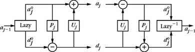
FIGURE 7.26 Predict and update decomposition of aj–1 into aj and dj, followed by the reconstruction of aj–1 with the same update and predict operators.
This fast biorthogonal wavelet transform (7.157) requires O(N) operations.
The reconstruction of aL from {dj}J≤j<L and aJ inverts these predict and update steps. For j = J, …, L + 1, it computes
Vanishing Moments
The predict and update filters are computed to create vanishing moments on the resulting wavelets. After the prediction applied to the lazy Diracs ψoj,m (x) = δ(x – xm), ϕoj,n(x) = δ(x – xn), the resulting wavelets and scaling functions derived from (7.248) and (7.249) are:
According to (7.250), the wavelet ψ1j,m has p1 vanishing moments if for each m, the p1 coefficients of {pj[m, n]}n solve the d1 × d1 linear system:
Following (7.253), after the update of the dual wavelet and the scaling functions, are
Theorem 7.28 proves that the vanishing moments of ψoj,m are transferred to ψ2j,m after the dual lifting step. According to (7.258), the dual wavelet ![]() has p2 vanishing moments if for each m the d2 coefficients of {uj[m, n]}n solve the d2 × d2 linear system:
has p2 vanishing moments if for each m the d2 coefficients of {uj[m, n]}n solve the d2 × d2 linear system:
The inner products Ikj (n) are computed iteratively with (7.259):
The recurrence is initialized at the finest scale j = L by setting IkL (n) = q(k) (xn), where xn ε Ω is the point associated to the index n ε GL. More elaborated initializations using quadrature formula can also be used [427].
Linear Splines 5/3 Biorthogonal Wavelets
Linear spline wavelets are obtained with a two-step lifting construction beginning from lazy wavelets. The one-dimensional grid Gj–1 is a uniform sampling at intervals 2j–1 and the two subgrids Gj and Cj correspond to even and odd subsampling. Figure 7.27 illustrates these embedded one-dimensional grids.

The lazy wavelet transform splits the coefficients aj–1 into two groups
The value of doj in Cj is predicted with a linear interpolation of neighbor values in Gj
This lifting step creates wavelets with two vanishing moments because this linear interpolation predicts exactly the values of polynomials of degree 0 and 1.
A symmetric update step computes
 (7.264)
To obtain two vanishing moments, the inner products ![]() are computed iteratively with (7.262), using two nonzero update coefficients uj [n, m − 2j–1] and uj [n, m + 2j–1] for each m. For k = 0 we get
are computed iteratively with (7.262), using two nonzero update coefficients uj [n, m − 2j–1] and uj [n, m + 2j–1] for each m. For k = 0 we get ![]() . Since t is antisymmetric, if this equation is valid for k = 0 and if uj[n, m − 2j–1] = uj[n, m + 2j–1], then it is valid for k = 1. Solving (7.261) for k = 0 gives uj[n, m − 2j–1] = uj[n, m + 2j–1] = 1/4 and thus,
. Since t is antisymmetric, if this equation is valid for k = 0 and if uj[n, m − 2j–1] = uj[n, m + 2j–1], then it is valid for k = 1. Solving (7.261) for k = 0 gives uj[n, m − 2j–1] = uj[n, m + 2j–1] = 1/4 and thus,
Figure 7.27 illustrates the succession of predict and update. One can verify (Exercise 7.20) that the resulting biorthogonal wavelets correspond to the spline biorthogonal wavelets computed with p1 = p2 = 2 vanishing moments (shown in Figure 7.15). The dual-scaling functions and wavelets are compactly supported linear splines. Higher-order biorthogonal spline wavelets are constructed with a prediction (7.263) and an update (7.264) providing more vanishing moments.
7.8.3 Quincunx Wavelet Bases
Separable two-dimensional wavelet bases are constructed in Section 7.7.2 from one-dimensional wavelet bases. They are implemented with separable filter banks that increase the scale by 2, by dividing the image grid in a coarse grid that keeps one point out of four, plus three detail grids of the same size and that correspond to three different wavelets. Other regular subsamplings of the image array lead to nonseparable wavelet bases. A quincunx subsampling divides the image grid into a coarse grid that keeps one point out of two and a detail grid of the same size that corresponds to a quincunx wavelet. Thus, the scale increases only by a factor 21/2. A quincunx wavelet is more isotropic than separable wavelets.
Biorthogonal or orthogonal quincunx wavelets are constructed with perfect reconstruction or conjugate mirror filters, defined with a quincunx subsampling, which yields conditions on their transfer functions [170, 253, 254, 431]. Kovacević and Sweldens [333] give a simple construction of biorthogonal quincunx wavelets from lazy wavelets, with a predict followed by an update lifting.
We denote by (a, b)* a transposed two-dimensional vector column. Embedded quincunx grids are defined by
Figure 7.28 shows two quincunx subsampled grids, depending on the parity of j. Each point n ε Gj and m ε Cj have four neighbors

where the set of shifts has the following four elements:
The simplest symmetric prediction operator on these grids is the symmetric averaging on the four neighbors, which performs a linear interpolation:
This prediction operator applied to lazy wavelets yields a wavelet that is orthogonal to constant and linear polynomial in ![]() 2, which gives p1 = 2 vanishing moments. The update operator is defined with the same symmetry on the four neighbors
2, which gives p1 = 2 vanishing moments. The update operator is defined with the same symmetry on the four neighbors
Choosing Λ = 1/4 satisfies the vanishing moments conditions (7.261) for constant and linear polynomials [333].
Figure 7.29 shows dual wavelets ![]() and
and ![]() at two consecutive scales 2j and 2j+1/2, corresponding to the predict and update operators (7.266) and (7.267). They have p2 = 2 vanishing moments and are nearly isotropic. The analyzing wavelets ψj,m also have p1 = 2 vanishing moments but are more irregular. The irregularity of analyzing wavelets is not a problem since the reconstruction is performed by dual wavelets. Wavelets with more vanishing moments are obtained by replacing the four-neighborhood linear interpolation (7.266) by higher-order polynomial interpolations [333]. Figure 7.29 shows the resulting dual wavelets
at two consecutive scales 2j and 2j+1/2, corresponding to the predict and update operators (7.266) and (7.267). They have p2 = 2 vanishing moments and are nearly isotropic. The analyzing wavelets ψj,m also have p1 = 2 vanishing moments but are more irregular. The irregularity of analyzing wavelets is not a problem since the reconstruction is performed by dual wavelets. Wavelets with more vanishing moments are obtained by replacing the four-neighborhood linear interpolation (7.266) by higher-order polynomial interpolations [333]. Figure 7.29 shows the resulting dual wavelets ![]() for p2 = 4 and p2 = 6, which correspond to wavelets ψj,m with as much vanishing moments p1 = p2, but which are more irregular. Increasing the number of vanishing moments improves the regularity of dual wavelets, but it reduces the stability of these biorthogonal bases, which limits their application.
for p2 = 4 and p2 = 6, which correspond to wavelets ψj,m with as much vanishing moments p1 = p2, but which are more irregular. Increasing the number of vanishing moments improves the regularity of dual wavelets, but it reduces the stability of these biorthogonal bases, which limits their application.

FIGURE 7.29 Quincunx dual wavelets ![]() and
and ![]() at two consecutive scales 2j and 2j+1/2 (first and second row) with progressively more vanishing moments.
at two consecutive scales 2j and 2j+1/2 (first and second row) with progressively more vanishing moments.
Figure 7.30 shows an example of quincunx wavelet image transform with p1 = 2 vanishing moments. It is computed with the fast lifting algorithm from Section 7.8.2 with the predict and update operators (7.266) and (7.267). The quasi-isotropic quincunx wavelet detects sharp transitions in all directions.
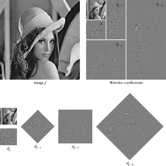
7.8.4 Wavelets on Bounded Domains and Surfaces
Processing three-dimensional surfaces and signals defined on surfaces is important in multimedia and computer graphics applications. Biorthogonal wavelets on triangulated meshes were introduced by Lounsbery et al. [354], and Schröder and Sweldens [427] improved these techniques with lifting schemes. Lifted wavelets are used to compress functions defined on a surface Ω ⊂ ![]() 3, and in particular on a sphere to process geographical data on Earth. The sphere is represented with a recursively subdivided three-dimensional mesh, and the signal is processed using lifted wavelets on this embedded mesh.
3, and in particular on a sphere to process geographical data on Earth. The sphere is represented with a recursively subdivided three-dimensional mesh, and the signal is processed using lifted wavelets on this embedded mesh.
Lifted wavelets are also defined on a two-dimensional parametric domain Ω with an arbitrary topology, to compress a three-dimensional surface S ⊂ ![]() 3, viewed as a mapping from Ω to
3, viewed as a mapping from Ω to ![]() 3. The surface is represented as a three-dimensional mesh, and the lifted wavelet transform computes three coefficients for each vertex of the mesh—one per coordinate. Denoising and compression of surfaces are then implemented by thresholding and quantizing these wavelet coefficients. Such multiresolution processings have applications in video games, where a large amount of three-dimensional surface data must be displayed in real time. Lifting wavelets also finds applications in computer-aided design, where surfaces are densely sampled to represent manufactured objects, and should be compressed to reduce the storage requirements.
3. The surface is represented as a three-dimensional mesh, and the lifted wavelet transform computes three coefficients for each vertex of the mesh—one per coordinate. Denoising and compression of surfaces are then implemented by thresholding and quantizing these wavelet coefficients. Such multiresolution processings have applications in video games, where a large amount of three-dimensional surface data must be displayed in real time. Lifting wavelets also finds applications in computer-aided design, where surfaces are densely sampled to represent manufactured objects, and should be compressed to reduce the storage requirements.
Semiregular Triangulation
A triangulation is a data structure frequently used to index points xn ε Ω on a surface. Embedded indexes n ε Gj with a triangulation topology are defined by recursively subdividing a coarse triangulated mesh.
For each scale j, a triangulation (Ej, Tj) is composed of edges Ej ⊂ Gj × Gj that link pairs of points on the grid, and triangles Tj ⊂ Gj × Gj × Gj. Each triangle of Tj is composed of three edges in Ej. These triangulations are supposed to be embedded using the 1:4 subdivision rule of each triangle, illustrated in Figure 7.31, as follows.
![]() For each edge e ε Ej, a midpoint γ(e) ε Gj–1 is added to the vertices
For each edge e ε Ej, a midpoint γ(e) ε Gj–1 is added to the vertices

FIGURE 7.31 (a) Iterated regular subdivision 1:4 of one triangle in four equal subtriangles. (b) Planar triangulation (G0, E0, T0) of a domain Ω in ![]() 2, successively refined with a 1:4 subdivision.
2, successively refined with a 1:4 subdivision.
![]() Each edge is subdivided into two finer edges
Each edge is subdivided into two finer edges
The subdivided set of edges is then
![]() Each triangle face f = (n0, n1, n2) ε Fj is subdivided into four faces
Each triangle face f = (n0, n1, n2) ε Fj is subdivided into four faces
The subdivided set of faces is then
Figure 7.31 shows an example of coarse planar triangulation with points xn in a domain Ω of ![]() 2.
2.
The semiregular mesh {Ej, Tj}j and the corresponding sample locations xn are usually computed from an input surface S, represented either with a parametric continuous function or with an unstructured set of polygons. This requires using a hierarchical remeshing process to compute the embedded triangulation [354]. Figure 7.32 shows an example of semiregular triangulation of a three-dimensional surface S, and in this case the points xn belong to a domain Ω that is the surface S in ![]() .
.

Wavelets to Process Functions on Surfaces
Let us consider a domain Ω ε ![]() 3 that is a three-dimensional surface, and each n ε Gj indexes a point xn ε Ω of the surface. Figure 7.33 shows the local labeling convention for the neighboring vertices in Gj of a given index m ε Cj in a butterfly neighborhood.
3 that is a three-dimensional surface, and each n ε Gj indexes a point xn ε Ω of the surface. Figure 7.33 shows the local labeling convention for the neighboring vertices in Gj of a given index m ε Cj in a butterfly neighborhood.

A predictor Pj is computed in this local neighborhood
 (7.268)
where the parameters Λi, μi, vi,j are calculated by solving (7.258) to obtain vanishing moments for a collection of low-degree polynomials {q(k)}0≤k<d1 [427].
The update operator ensures that the dual wavelets have one vanishing moment. It is calculated on the direct neighbors in Cj of each point n ε Gj:
The update operator is parameterized as follows:
where each Λn is computed to solve the system (7.261) to obtain vanishing moments. This requires the iterative computation of the moments Ikj (n), as explained in (7.262), with an initialization IkL (n) = 1 at the finest scale L of the mesh. In a perfectly regular triangulation, where all the points have six neighbors, a constant weight Λn = Λ can be used, and one can check that Λn = 1/24 guarantees one vanishing moment.
Processing signals on a sphere is an important application of these wavelets on surfaces [427]. The triangulated mesh is obtained by a 1:4 subdivision of a regular polyhedron, for instance a tetrahedron. The positions of the points xn for n ε Gj are defined recursively by projecting midpoints of the edges on the sphere:
The signal ![]() is defined on the finest mesh GL.
is defined on the finest mesh GL.
A nonlinear approximation is obtained by setting to zero wavelet coefficients that satisfy |〈f, ψj,m〉 | ≤ T ‖ψj,m ‖ where T is a given threshold. The value of ‖ψj,m‖ can be approximated from the size of its support ![]() [427]. Figure 7.34 shows an example of such a nonlinear approximation with an image of Earth defined as a function on the sphere.
[427]. Figure 7.34 shows an example of such a nonlinear approximation with an image of Earth defined as a function on the sphere.

Wavelets to Process Surfaces
A three-dimensional surface S ⊂ ![]() 3 is represented as a mapping from a two-dimensional parameter domain Ω to
3 is represented as a mapping from a two-dimensional parameter domain Ω to ![]() 3. This surface is discretized with a semiregular mesh {Gj, Ej, Tj}L≤j≤0, and thus Ω can be chosen as the finest grid GL viewed as an abstract domain. The surface is a discrete mapping from Ω = GL to
3. This surface is discretized with a semiregular mesh {Gj, Ej, Tj}L≤j≤0, and thus Ω can be chosen as the finest grid GL viewed as an abstract domain. The surface is a discrete mapping from Ω = GL to ![]() 3 that assigns to each n ε Ω three values (f1 [n], f2 [n], f3 [n]) ε S, which is a position in the three-dimensional space.
3 that assigns to each n ε Ω three values (f1 [n], f2 [n], f3 [n]) ε S, which is a position in the three-dimensional space.
Processing the discrete surface is equivalent to processing the three signals (f1, f2, f3) where each ![]() is defined on the finest grid GL. Since points in the parametric domain Ω do not have positions in Euclidean space, the notion of vanishing moments is not well defined, and the predict operator is computed using weights that are calculated as if the faces of the mesh were equilateral triangles. One can verify that the resulting parameters of the predict operator (7.268) are Λi = 1/2, μi = 1/4, and vi,j = − 1/16 [427]. Figure 7.35 shows the corresponding wavelets on a subdivided equilateral triangle.
is defined on the finest grid GL. Since points in the parametric domain Ω do not have positions in Euclidean space, the notion of vanishing moments is not well defined, and the predict operator is computed using weights that are calculated as if the faces of the mesh were equilateral triangles. One can verify that the resulting parameters of the predict operator (7.268) are Λi = 1/2, μi = 1/4, and vi,j = − 1/16 [427]. Figure 7.35 shows the corresponding wavelets on a subdivided equilateral triangle.
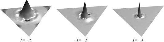
FIGURE 7.35 Example of dual wavelets ![]() for x on a subdivided equilateral triangle. The height over the triangle indicates the value of the wavelet.
for x on a subdivided equilateral triangle. The height over the triangle indicates the value of the wavelet.
These wavelets are used to compress each of the three signals ![]() by uniformly quantizing the normalized coefficients 〈fi, ψj,m〉 / ‖ ψj,m ‖. The resulting set of quantized coefficients are within strings with an entropy coder algorithm, described in Section 10.2.1. The quantization and coding of sparse signal representation is described in Section 10.4.
by uniformly quantizing the normalized coefficients 〈fi, ψj,m〉 / ‖ ψj,m ‖. The resulting set of quantized coefficients are within strings with an entropy coder algorithm, described in Section 10.2.1. The quantization and coding of sparse signal representation is described in Section 10.4.
Figure 7.36 shows an example of three-dimensional surface approximation using biorthogonal wavelets on triangulated meshes. Wavelet coders based on lifting offer state-of-the-art results in surface compression [327]. There is no control on the Riesz bounds of the lifted wavelet basis, because the lifted basis depends on the surface properties, but good approximation results are obtained.

7.8.5 Faster Wavelet Transform with Lifting
Lifting is used to reduce the number of operations of a one-dimensional fast wavelet transform by factorizing the filter bank convolutions. It also reduces the memory requirements by implementing all operations, in place, within the input signal array.
Before the introduction of liftings for wavelet design, the factorization of filter bank convolutions was studied as paraunitary filter banks by Vaidyanathan [68] and other signal-processing researchers. Instead of implementing a filter bank with convolutions and subsamplings, specific filters are designed for even and odd signal coefficients. These filters are shown to be factorized as a succession of elementary operators that correspond to the predict and update operators of a lifting. This filtering architecture reduces by up to 2 the number of additions and multiplications, and simplifies folding border treatments for symmetric wavelets.
The fast wavelet transform algorithm in Sections 7.3.1 and 7.3.2 decomposes iteratively the scaling coefficients aj [n] at a scale 2j into larger-scale coefficients aj+1 [n] and detail wavelet coefficients dj+1 [n], with convolutions and subsampling using two filters h and g. According to (7.157),
with ![]() and
and ![]() . The reconstruction is performed with the dual filters
. The reconstruction is performed with the dual filters ![]() and
and ![]() according to (7.158),
according to (7.158),
Sweldens and Daubechies [199] proved that the convolutions and subsamplings (7.270) can be implemented with a succession of lifting steps and the reconstruction (7.271) by inverting these liftings.
Each uniform one-dimensional signal sampling grid Gj of aj [n] is divided into even samples in Gj+1 and odd samples in Cj where aj+1 and dj+1 are, respectively, defined. Starting from the lazy wavelet transform that splits even and odd samples of aj [n], K couples of predict and update convolution operators {P(k), U(k)}1≤k≤K are sequentially applied. Each predict operator P(k) corresponds to a filter p(k) [n] and each update operator to a filter u(k) [m]. The filters have a small support of typically two coefficients. They are computed from the biorthogonal filters ![]() with a Euclidean division algorithm [199]. A final scaling step renormalizes the filter coefficients.
with a Euclidean division algorithm [199]. A final scaling step renormalizes the filter coefficients.
Let aL [n] be the input finest-scale signal for n ε GL. The lifting implementation of a fast wavelet transform proceeds as follow. For j = L + 1,…, J:
The fast inverse wavelet transform recovers aL from the set of wavelet coefficients {dj}0≤j<L and aJ by inverting these predict and update operators. For j = J,…, L + 1:
1. Inverse scaling: Initialize d(K)j = ζ dj and a(K)j = aj / ζ. The following steps, 2 and 3, are performed for k = K,…, 1.
One can verify (Exercise 7.21) that this implementation divides the number of operations by up to a factor of 2, compared to direct convolutions and subsamplings calculated in (7.270) and (7.271). Moreover, this algorithm proceeds “in place,” which means that it only uses the memory of the original array GL with coefficients that are progressively modified by the lifting operations; it then stores the resulting wavelet coefficients. Similarly the reconstruction operates in place by reconstructing progressively the coefficients in the array GL.
Symmetric Lifting on the Interval
The lifting implementation is described in more detail for symmetric wavelets on an interval, corresponding to symmetric biorthogonal filters ![]() . Predict and update convolutions are modified at the boundaries to implement folding boundary conditions.
. Predict and update convolutions are modified at the boundaries to implement folding boundary conditions.
The input sampling grid GL has N = 2−L samples at integer positions 0 ≤ n < N. The embedded subgrids at scales 0 ≥ 2j > 2L are
The resulting lifting operators {P(k), U(k)}1≤k≤K are two-tap symmetric convolution operators. A prediction of parameter Λ is defined by
An update of parameter μ is defined as
At the interval boundaries, the predict and update operators must be modified for m = N – N 2j–1 in (7.273) and n = 0 in (7.274), because one of the two neighbors falls outside the grids Gj and Cj.
Symmetric boundary conditions, described in Section 7.5.2, are implemented with a folding, which leads to the following definition of boundary predict and update operators:
This ensures that the lifting operators have one vanishing moment, and that the resulting boundary wavelets also have one vanishing moment.
Factorization of 5/3 and 9/7 Biorthogonal Wavelets
The 9/7 biorthogonal and 5/3 wavelets in Figure 7.15 are recommended for image compression in JPEG-2000 and are often used in wavelet image-processing applications. The 5/3 biorthogonal wavelet has p1 = p2 = 2 vanishing moments, while the 9/7 wavelet has p1 = p2 = 4 vanishing moments.
The 5/3 wavelet transform is implemented with K = 1 pair of predict and update steps, presented in Section 7.8.2. They correspond to
The 9/7 wavelet transform is implemented with K = 2 pairs of predict and update steps defined as
7.9 EXERCISES
7.1. 2 Let h be a conjugate mirror filter associated to a scaling function ϕ.
7.2. 2Prove that ![]() = 1 if ϕ is an orthogonal scaling function.
= 1 if ϕ is an orthogonal scaling function.
7.3. 2Let ϕm be the Battle-Lemarié scaling function of degree m defined in (7.18). Let ϕ be the Shannon scaling function defined by ![]() . Prove that
. Prove that ![]() .
.
7.4. 3Suppose that h [n] is nonzero only for 0 ≤ n < K. We denote ![]() . The scaling equation is ϕ (t) =
. The scaling equation is ϕ (t) = ![]() .
.
with ϕ0 = 1[0,1], and ak [n] = 〈ϕk (t), ϕk (t – n)〉.
7.6. 3 Let b [n] =f (N−1n) with 2L = N−1 and f ε VL. We want to recover aL [n] = 〈f, ϕL,n〉 from b [n] to compute the wavelet coefficients of f with Theorem 7.10.

then aL can be calculated from b with a stable filter ϕ−1L [n].
7.7. 2 Quadrature mirror filters. We define a multirate filter bank with four filters h, g, ![]() , and
, and ![]() , which decomposes a signal a0 [n]
, which decomposes a signal a0 [n]
a1 [n] = a0 ![]() h [2n], d1 [n] = a0
h [2n], d1 [n] = a0 ![]() g [2n].
g [2n].
Using the notation (7.101), we reconstruct
7.8. 7.8 1 Let f be a function of support [0, 1] that is equal to different polynomials of degree q on the intervals {[τk, τk+1]}0≤k<K with τ0 = 0 and τK = 1. Let ψ be a Daubechies wavelet with p vanishing moments. If q < p, compute the number of nonzero wavelet coefficients 〈 f, ψj,n 〉 at a fixed scale 2j. How should we choose p to minimize this number? If q > p, what is the maximum number of nonzero wavelet coefficients 〈 f, ψj,n 〉 at a fixed scale 2ĵ
7.9. 7.9 2 Let θ be a box spline of degree m obtained by m + 1 convolutions of 1[0,1] with itself.

7.10. 1 Prove that if {ψj,n}(j,n) ε![]() 2 is an orthonormal basis of L2(
2 is an orthonormal basis of L2(![]() ), then for all ω ε
), then for all ω ε ![]() – {0},
– {0}, ![]() . Find an example showing that the converse is not true.
. Find an example showing that the converse is not true.
Prove that {ψj,n}(j,n) ε![]() 2 is an orthonormal basis of L2(
2 is an orthonormal basis of L2(![]() ). Prove that ψ is not associated to a scaling function ϕ that generates a multiresolution approximation.
). Prove that ψ is not associated to a scaling function ϕ that generates a multiresolution approximation.
7.12. 2 Express the Coiflet property (7.99) as an equivalent condition on the conjugate mirror filter ![]() .
.
7.13. 1 Prove that ψ (t) has p vanishing moments if and only if, for all j > 0, the discrete wavelets ψj [n] defined in (7.140) have p discrete vanishing moments
7.14. 2 Let ψ (t) be a compactly supported wavelet calculated with Daubechies conjugate mirror filters (h, g). Let ψ′j,n (t) = 2−j/2ψ′(2−jt – n) be the derivative wavelets.
7.15. 3 Let ψ(t) be a compactly supported wavelet calculated with Daubechies conjugate mirror filters (h, g). Let ![]() . We verify that
. We verify that ![]() is an almost analytic wavelet.
is an almost analytic wavelet.
show that we can modify the fast wavelet transform algorithm to compute the “analytic” wavelet coefficients 〈 f, ψaj,n 〉 by inserting a new filter.
Let ψkj,n (x) = 2−j ψk (2−j x – n) for n ε ![]() 2. Modify the separable wavelet filter bank algorithm from Section 7.7.3 to compute the “analytic” wavelet coefficients 〈 f ψkj,n 〉.
2. Modify the separable wavelet filter bank algorithm from Section 7.7.3 to compute the “analytic” wavelet coefficients 〈 f ψkj,n 〉.
7.16. 2 Multiwavelets. We define the following two scaling functions:

7.17. 3 Let frepl be the folded function defined in (7.179).
7.18. 3 A recursive filter has a Fourier transform that is a ratio of trigonometric polynomials as in (2.31).
7.19. 2 Balancing. Suppose that h, ![]() define a pair of perfect reconstruction filters satisfying (7.124).
define a pair of perfect reconstruction filters satisfying (7.124).
defines a new pair of perfect reconstruction filters. Verify that ![]() and
and ![]() have, respectively, one more and one less zero at π than
have, respectively, one more and one less zero at π than ![]() and
and ![]() [63].
[63].
Compute hnew and ![]() as well as the corresponding biorthogonal wavelets ψnew,
as well as the corresponding biorthogonal wavelets ψnew, ![]() , after one balancing and again after a second balancing.
, after one balancing and again after a second balancing.
7.20. 1 Compute numerically the wavelets and scaling functions associated to the predict and update lifting steps (7.264) and (7.265). Verify that you obtain the 5/3 wavelets displayed in Figure 7.15.
7.21. 1 Give the reduction of the number of operations when implementing a fast wavelet transform with 5/3 and 7/9 biorthogonal wavelets with the lifting algorithm described in Section 7.8.5, compared with a direct implementation with (7.270) and (7.271) by using the coefficients in Table 7.4.
7.22. 1 For a Deslauriers-Dubuc interpolation wavelet of degree 3, compute the dual wavelet ![]() in (7.212), which is a sum of Diracs. Verify that it has four vanishing moments.
in (7.212), which is a sum of Diracs. Verify that it has four vanishing moments.
7.23. 2 Prove that a Deslauriers-Dubuc interpolation function of degree 2p − 1 converges to a sinc function when p goes to + ∞.
7.24. 3 Let ϕ be an autocorrelation scaling function that reproduces polynomials of degree p − 1 as in (7.198). Prove that if f is uniformly Lipschitz α, then under the same hypotheses as in Theorem 7.22, there exists K > 0 such that
7.25. 2 Let ϕ (t) be an interpolation function that generates an interpolation wavelet basis of C0 (![]() ). Construct a separable interpolation wavelet basis of the space C0 (
). Construct a separable interpolation wavelet basis of the space C0 (![]() p) of uniformly continuous p-dimensional signals f (x1, …, xp). Hint: Construct 2p − 1 interpolation wavelets by appropriately translating ϕ (x1) … ϕ(xp).
p) of uniformly continuous p-dimensional signals f (x1, …, xp). Hint: Construct 2p − 1 interpolation wavelets by appropriately translating ϕ (x1) … ϕ(xp).
7.26. 3 Fractional Brownian. Let ψ (t) be a compactly supported wavelet with p vanishing moments that generates an orthonormal basis of L2(![]() ). The covariance of a fractional Brownian motion BH (t) is given by (6.86).
). The covariance of a fractional Brownian motion BH (t) is given by (6.86).
7.27. 2 Image mosaic. Let f0 [n1, n2] and f1 [n1, n2] be two square images of N pixels. We want to merge the center of f0 [n1, n2] for N1/2 / 4 ≤ n1, n2 < 3N1/2 / 4 in the center of f1. Compute numerically the wavelet coefficients of f0 and f1. At each scale 2j and orientation 1 ≤ k ≤ 3, replace the 2−2j/4 wavelet coefficients corresponding to the center of f1 by the wavelet coefficients of f0. Reconstruct an image from this manipulated wavelet representation. Explain why the image f0 seems to be merged in f1, without the strong boundary effects that are obtained when directly replacing the pixels of f1 by the pixels of f0.
7.28. 3 Foveal vision. A foveal image has a maximum resolution at the center, with a resolution that decreases linearly as a function of the distance to the center. Show that one can construct an approximate foveal image by keeping a constant number of nonzero wavelet coefficients at each scale 2j. Implement this algorithm numerically.
7.29. 2 High contrast. We consider a color image specified by three color channels: red r [n], green g [n], and blue b [n]. The intensity image (r + g + b) /3 averages the variations of the three color channels. To create a high-contrast image f, for each wavelet ψkj,n we set 〈f, ψkj,n〉 to be the coefficient among 〈r, ψkj,n〉, 〈g, ψkj,n〉, and 〈b, ψkj,n〉, which has the maximum amplitude. Implement this algorithm numerically and evaluate its performance for different types of multispectral images. How does the choice of ψ affect the results?