
CHAPTER 1 Sparse Representations
Signals carry overwhelming amounts of data in which relevant information is often more difficult to find than a needle in a haystack. Processing is faster and simpler in a sparse representation where few coefficients reveal the information we are looking for. Such representations can be constructed by decomposing signals over elementary waveforms chosen in a family called a dictionary. But the search for the Holy Grail of an ideal sparse transform adapted to all signals is a hopeless quest. The discovery of wavelet orthogonal bases and local time-frequency dictionaries has opened the door to a huge jungle of new transforms. Adapting sparse representations to signal properties, and deriving efficient processing operators, is therefore a necessary survival strategy.
An orthogonal basis is a dictionary of minimum size that can yield a sparse representation if designed to concentrate the signal energy over a set of few vectors. This set gives a geometric signal description. Efficient signal compression and noise-reduction algorithms are then implemented with diagonal operators computed with fast algorithms. But this is not always optimal.
In natural languages, a richer dictionary helps to build shorter and more precise sentences. Similarly, dictionaries of vectors that are larger than bases are needed to build sparse representations of complex signals. But choosing is difficult and requires more complex algorithms. Sparse representations in redundant dictionaries can improve pattern recognition, compression, and noise reduction, but also the resolution of new inverse problems. This includes superresolution, source separation, and compressive sensing.
This first chapter is a sparse book representation, providing the story line and the main ideas. It gives a sense of orientation for choosing a path to travel.
1.1 COMPUTATIONAL HARMONIC ANALYSIS
Fourier and wavelet bases are the journey’s starting point. They decompose signals over oscillatory waveforms that reveal many signal properties and provide a path to sparse representations. Discretized signals often have a very large size N ≥ 106, and thus can only be processed by fast algorithms, typically implemented with O(N log N) operations and memories. Fourier and wavelet transforms illustrate the strong connection between well-structured mathematical tools and fast algorithms.
1.1.1 The Fourier Kingdom
The Fourier transform is everywhere in physics and mathematics because it diagonalizes time-invariant convolution operators. It rules over linear time-invariant signal processing, the building blocks of which are frequency filtering operators.
Fourier analysis represents any finite energy function f(t) as a sum of sinusoidal waves ![]() :
:
The amplitude ![]() of each sinusoidal wave eiwt is equal to its correlation with f, also called Fourier transform:
of each sinusoidal wave eiwt is equal to its correlation with f, also called Fourier transform:
The more regular f(t), the faster the decay of the sinusoidal wave amplitude ![]() when frequency ω increases.
when frequency ω increases.
When f(t) is defined only on an interval, say [0, 1], then the Fourier transform becomes a decomposition in a Fourier orthonormal basis {ei2πmt}m∈![]() of L2[0, 1]. If f(t) is uniformly regular, then its Fourier transform coefficients also have a fast decay when the frequency 2πm increases, so it can be easily approximated with few low-frequency Fourier coefficients. The Fourier transform therefore defines a sparse representation of uniformly regular functions.
of L2[0, 1]. If f(t) is uniformly regular, then its Fourier transform coefficients also have a fast decay when the frequency 2πm increases, so it can be easily approximated with few low-frequency Fourier coefficients. The Fourier transform therefore defines a sparse representation of uniformly regular functions.
Over discrete signals, the Fourier transform is a decomposition in a discrete orthogonal Fourier basis {ei2π kn/N}0≤ k<N of ![]() N, which has properties similar to a Fourier transform on functions. Its embedded structure leads to fast Fourier transform (FFT) algorithms, which compute discrete Fourier coefficients with O(N log N) instead of N2. This FFT algorithm is a cornerstone of discrete signal processing.
N, which has properties similar to a Fourier transform on functions. Its embedded structure leads to fast Fourier transform (FFT) algorithms, which compute discrete Fourier coefficients with O(N log N) instead of N2. This FFT algorithm is a cornerstone of discrete signal processing.
As long as we are satisfied with linear time-invariant operators or uniformly regular signals, the Fourier transform provides simple answers to most questions. Its richness makes it suitable for a wide range of applications such as signal transmissions or stationary signal processing. However, to represent a transient phenomenon—a word pronounced at a particular time, an apple located in the left corner of an image—the Fourier transform becomes a cumbersome tool that requires many coefficients to represent a localized event. Indeed, the support of ![]() covers the whole real line, so
covers the whole real line, so ![]() depends on the values f(t) for all times t ∈
depends on the values f(t) for all times t ∈ ![]() . This global “mix” of information makes it difficult to analyze or represent any local property of f(t) from
. This global “mix” of information makes it difficult to analyze or represent any local property of f(t) from ![]() .
.
1.1.2 Wavelet Bases
Wavelet bases, like Fourier bases, reveal the signal regularity through the amplitude of coefficients, and their structure leads to a fast computational algorithm. However, wavelets are well localized and few coefficients are needed to represent local transient structures. As opposed to a Fourier basis, a wavelet basis defines a sparse representation of piecewise regular signals, which may include transients and singularities. In images, large wavelet coefficients are located in the neighborhood of edges and irregular textures.
The story began in 1910, when Haar [291] constructed a piecewise constant function

the dilations and translations of which generate an orthonormal basis
of the space L2(![]() ) of signals having a finite energy
) of signals having a finite energy
Let us write 〈f, g〉 = ![]() f(t)g*(t) dt—the inner product in L2(
f(t)g*(t) dt—the inner product in L2(![]() ). Any finite energy signal f can thus be represented by its wavelet inner-product coefficients
). Any finite energy signal f can thus be represented by its wavelet inner-product coefficients
and recovered by summing them in this wavelet orthonormal basis:
 (1.3)
(1.3)Each Haar wavelet ![]() has a zero average over its support [2jn, 2j(n + 1)]. If f is locally regular and 2j is small, then it is nearly constant over this interval and the wavelet coefficient
has a zero average over its support [2jn, 2j(n + 1)]. If f is locally regular and 2j is small, then it is nearly constant over this interval and the wavelet coefficient ![]() is nearly zero. This means that large wavelet coefficients are located at sharp signal transitions only.
is nearly zero. This means that large wavelet coefficients are located at sharp signal transitions only.
With a jump in time, the story continues in 1980, when StröUmberg [449] found a piecewise linear function ψ that also generates an orthonormal basis and gives better approximations of smooth functions. Meyer was not aware of this result, and motivated by the work of Morlet and Grossmann over continuous wavelet transform, he tried to prove that there exists no regular wavelet ψ that generates an orthonormal basis. This attempt was a failure since he ended up constructing a whole family of orthonormal wavelet bases, with functions ψ that are infinitely continuously differentiable [375]. This was the fundamental impulse that led to a widespread search for new orthonormal wavelet bases, which culminated in the celebrated Daubechies wavelets of compact support [194].
The systematic theory for constructing orthonormal wavelet bases was established by Meyer and Mallat through the elaboration of multiresolution signal approximations [362], as presented in Chapter 7. It was inspired by original ideas developed in computer vision by Burt and Adelson [126] to analyze images at several resolutions. Digging deeper into the properties of orthogonal wavelets and multiresolution approximations brought to light a surprising link with filter banks constructed with conjugate mirror filters, and a fast wavelet transform algorithm decomposing signals of size N with O(N) operations [361].
Filter Banks
Motivated by speech compression, in 1976 Croisier, Esteban, and Galand [189] introduced an invertible filter bank, which decomposes a discrete signal f[n] into two signals of half its size using a filtering and subsampling procedure. They showed that f[n] can be recovered from these subsampled signals by canceling the aliasing terms with a particular class of filters called conjugate mirror filters. This breakthrough led to a 10-year research effort to build a complete filter bank theory. Necessary and sufficient conditions for decomposing a signal in subsampled components with a filtering scheme, and recovering the same signal with an inverse transform, were established by Smith and Barnwell [444], Vaidyanathan [469], and Vetterli [471].
The multiresolution theory of Mallat [362] and Meyer [44] proves that any conjugate mirror filter characterizes a wavelet ψ that generates an orthonormal basis of ![]() , and that a fast discrete wavelet transform is implemented by cascading these conjugate mirror filters [361]. The equivalence between this continuous time wavelet theory and discrete filter banks led to a new fruitful interface between digital signal processing and harmonic analysis, first creating a culture shock that is now well resolved.
, and that a fast discrete wavelet transform is implemented by cascading these conjugate mirror filters [361]. The equivalence between this continuous time wavelet theory and discrete filter banks led to a new fruitful interface between digital signal processing and harmonic analysis, first creating a culture shock that is now well resolved.
Continuous versus Discrete and Finite
Originally many signal processing engineers were wondering what is the point of considering wavelets and signals as functions, since all computations are performed over discrete signals with conjugate mirror filters. Why bother with the convergence of infinite convolution cascades if in practice we only compute a finite number of convolutions? Answering these important questions is necessary in order to understand why this book alternates between theorems on continuous time functions and discrete algorithms applied to finite sequences.
A short answer would be “simplicity.” In ![]() , a wavelet basis is constructed by dilating and translating a single function ψ. Several important theorems relate the amplitude of wavelet coefficients to the local regularity of the signal f. Dilations are not defined over discrete sequences, and discrete wavelet bases are therefore more complex to describe. The regularity of a discrete sequence is not well defined either, which makes it more difficult to interpret the amplitude of wavelet coefficients. A theory of continuous-time functions gives asymptotic results for discrete sequences with sampling intervals decreasing to zero. This theory is useful because these asymptotic results are precise enough to understand the behavior of discrete algorithms.
, a wavelet basis is constructed by dilating and translating a single function ψ. Several important theorems relate the amplitude of wavelet coefficients to the local regularity of the signal f. Dilations are not defined over discrete sequences, and discrete wavelet bases are therefore more complex to describe. The regularity of a discrete sequence is not well defined either, which makes it more difficult to interpret the amplitude of wavelet coefficients. A theory of continuous-time functions gives asymptotic results for discrete sequences with sampling intervals decreasing to zero. This theory is useful because these asymptotic results are precise enough to understand the behavior of discrete algorithms.
But continuous time or space models are not sufficient for elaborating discrete signal-processing algorithms. The transition between continuous and discrete signals must be done with great care to maintain important properties such as orthogonality. Restricting the constructions to finite discrete signals adds another layer of complexity because of border problems. How these border issues affect numerical implementations is carefully addressed once the properties of the bases are thoroughly understood.
Wavelets for Images
Wavelet orthonormal bases of images can be constructed from wavelet orthonormal bases of one-dimensional signals. Three mother wavelets ψ1(x), ψ2(x), and ψ3(x), with x = (x1, x2) ∈ ![]() 2, are dilated by 2j and translated by 2j n with n = (n1, n2) ∈
2, are dilated by 2j and translated by 2j n with n = (n1, n2) ∈ ![]() 2. This yields an orthonormal basis of the space L2(
2. This yields an orthonormal basis of the space L2(![]() 2) of finite energy functions f(x) = f(x1, x2):
2) of finite energy functions f(x) = f(x1, x2):
The support of a wavelet ![]() is a square of width proportional to the scale 2j. Two-dimensional wavelet bases are discretized to define orthonormal bases of images including N pixels. Wavelet coefficients are calculated with the fast O(N) algorithm described in Chapter 7.
is a square of width proportional to the scale 2j. Two-dimensional wavelet bases are discretized to define orthonormal bases of images including N pixels. Wavelet coefficients are calculated with the fast O(N) algorithm described in Chapter 7.
Like in one dimension, a wavelet coefficient ![]() has a small amplitude if f(x) is regular over the support of
has a small amplitude if f(x) is regular over the support of ![]() . It has a large amplitude near sharp transitions such as edges. Figure 1.1(b) is the array of N wavelet coefficients. Each direction k and scale 2j corresponds to a subimage, which shows in black the position of the largest coefficients above a threshold:
. It has a large amplitude near sharp transitions such as edges. Figure 1.1(b) is the array of N wavelet coefficients. Each direction k and scale 2j corresponds to a subimage, which shows in black the position of the largest coefficients above a threshold: ![]()

FIGURE 1.1 (a) Discrete image f[n] of N = 2562 pixels. (b) Array of N orthogonal wavelet coefficients 〈f, ψkj,n〉 for k = 1, 2, 3, and 4 scales 2j; black points correspond to |〈f, ψkj,n〉| >T. (c) Linear approximation from the N/16 wavelet coefficients at the three largest scales. (d) Nonlinear approximation from the M = N/16 wavelet coefficients of largest amplitude shown in (b).
1.2 APPROXIMATION AND PROCESSING IN BASES
Analog-to-digital signal conversion is the first step of digital signal processing. Chapter 3 explains that it amounts to projecting the signal over a basis of an approximation space. Most often, the resulting digital representation remains much too large and needs to be further reduced. A digital image typically includes more than 106 samples and a CD music recording has 40 × 103 samples per second. Sparse representations that reduce the number of parameters can be obtained by thresholding coefficients in an appropriate orthogonal basis. Efficient compression and noise-reduction algorithms are then implemented with simple operators in this basis.
Stochastic versus Deterministic Signal Models
A representation is optimized relative to a signal class, corresponding to all potential signals encountered in an application. This requires building signal models that carry available prior information.
A signal f can be modeled as a realization of a random process F, the probability distribution of which is known a priori. A Bayesian approach then tries to minimize the expected approximation error. Linear approximations are simpler because they only depend on the covariance. Chapter 9 shows that optimal linear approximations are obtained on the basis of principal components that are the eigenvectors of the covariance matrix. However, the expected error of nonlinear approximations depends on the full probability distribution of F. This distribution is most often not known for complex signals, such as images or sounds, because their transient structures are not adequately modeled as realizations of known processes such as Gaussian ones.
To optimize nonlinear representations, weaker but sufficiently powerful deterministic models can be elaborated. A deterministic model specifies a set Θ, where the signal belongs. This set is defined by any prior information—for example, on the time-frequency localization of transients in musical recordings or on the geometric regularity of edges in images. Simple models can also define Θ as a ball in a functional space, with a specific regularity norm such as a total variation norm. A stochastic model is richer because it provides the probability distribution in Θ. When this distribution is not available, the average error cannot be calculated and is replaced by the maximum error over Θ. Optimizing the representation then amounts to minimizing this maximum error, which is called a minimax optimization.
1.2.1 Sampling with Linear Approximations
Analog-to-digital signal conversion is most often implemented with a linear approximation operator that filters and samples the input analog signal. From these samples, a linear digital-to-analog converter recovers a projection of the original analog signal over an approximation space whose dimension depends on the sampling density. Linear approximations project signals in spaces of lowest possible dimensions to reduce computations and storage cost, while controlling the resulting error.
Sampling Theorems
Let us consider finite energy signals ![]() dx of finite support, which is normalized to [0, 1] or [0, 1]2 for images. A sampling process implements a filtering of
dx of finite support, which is normalized to [0, 1] or [0, 1]2 for images. A sampling process implements a filtering of ![]() and a uniform sampling to output a discrete signal:
and a uniform sampling to output a discrete signal:
In two dimensions, n = (n1, n2) and x = (x1, x2). These filtered samples can also be written as inner products:
with ![]() . Chapter 3 explains that φs is chosen, like in the classic Shannon-Whittaker sampling theorem, so that a family of functions
. Chapter 3 explains that φs is chosen, like in the classic Shannon-Whittaker sampling theorem, so that a family of functions ![]() is a basis of an appropriate approximation space UN. The best linear approximation of
is a basis of an appropriate approximation space UN. The best linear approximation of ![]() in UN recovered from these samples is the orthogonal projection
in UN recovered from these samples is the orthogonal projection ![]() N of f in UN, and if the basis is orthonormal, then
N of f in UN, and if the basis is orthonormal, then
 (1.4)
(1.4)A sampling theorem states that if ![]() ∈ UN then
∈ UN then ![]() so (1.4) recovers
so (1.4) recovers ![]() from the measured samples. Most often,
from the measured samples. Most often, ![]() does not belong to this approximation space. It is called aliasing in the context of Shannon-Whittaker sampling, where UN is the space of functions having a frequency support restricted to the N lower frequencies. The approximation error
does not belong to this approximation space. It is called aliasing in the context of Shannon-Whittaker sampling, where UN is the space of functions having a frequency support restricted to the N lower frequencies. The approximation error ![]() must then be controlled.
must then be controlled.
Linear Approximation Error
The approximation error is computed by finding an orthogonal basis ![]() of the whole analog signal space L2[0, 1]2, with the first N vector
of the whole analog signal space L2[0, 1]2, with the first N vector ![]() that defines an orthogonal basis of UN. Thus, the orthogonal projection on UN can be rewritten as
that defines an orthogonal basis of UN. Thus, the orthogonal projection on UN can be rewritten as

Since ![]() , the approximation error is the energy of the removed inner products:
, the approximation error is the energy of the removed inner products:

This error decreases quickly when N increases if the coefficient amplitudes ![]() have a fast decay when the index m increases. The dimension N is adjusted to the desired approximation error.
have a fast decay when the index m increases. The dimension N is adjusted to the desired approximation error.
Figure 1.1(a) shows a discrete image f[n] approximated with N = 2562 pixels. Figure 1.1(c) displays a lower-resolution image fN/16 projected on a space UN/16 of dimension N/16, generated by N/16 large-scale wavelets. It is calculated by setting all the wavelet coefficients to zero at the first two smaller scales. The approximation error is ‖f – fN/16‖2/‖f‖2 = 14 × 10−3. Reducing the resolution introduces more blur and errors. A linear approximation space UN corresponds to a uniform grid that approximates precisely uniform regular signals. Since images ![]() are often not uniformly regular, it is necessary to measure it at a high-resolution N. This is why digital cameras have a resolution that increases as technology improves.
are often not uniformly regular, it is necessary to measure it at a high-resolution N. This is why digital cameras have a resolution that increases as technology improves.
1.2.2 Sparse Nonlinear Approximations
Linear approximations reduce the space dimensionality but can introduce important errors when reducing the resolution if the signal is not uniformly regular, as shown by Figure 1.1(c). To improve such approximations, more coefficients should be kept where needed—not in regular regions but near sharp transitions and edges. This requires defining an irregular sampling adapted to the local signal regularity. This optimized irregular sampling has a simple equivalent solution through nonlinear approximations in wavelet bases.
Nonlinear approximations operate in two stages. First, a linear operator approximates the analog signal ![]() with N samples written
with N samples written ![]() . Then, a nonlinear approximation of f[n] is computed to reduce the N coefficients f[n] to M
. Then, a nonlinear approximation of f[n] is computed to reduce the N coefficients f[n] to M ![]() N coefficients in a sparse representation.
N coefficients in a sparse representation.
The discrete signal f can be considered as a vector of ![]() N. Inner products and norms in
N. Inner products and norms in ![]() N are written
N are written

To obtain a sparse representation with a nonlinear approximation, we choose a new orthonormal basis B = {gm[n]}m∈γ of ![]() N, which concentrates the signal energy as much as possible over few coefficients. Signal coefficients {〈f, gm〉}m∈γ are computed from the N input sample values f[n] with an orthogonal change of basis that takes N2 operations in nonstructured bases. In a wavelet or Fourier bases, fast algorithms require, respectively, O(N) and O(N log2 N) operations.
N, which concentrates the signal energy as much as possible over few coefficients. Signal coefficients {〈f, gm〉}m∈γ are computed from the N input sample values f[n] with an orthogonal change of basis that takes N2 operations in nonstructured bases. In a wavelet or Fourier bases, fast algorithms require, respectively, O(N) and O(N log2 N) operations.
Approximation by Thresholding
For M < N, an approximation fM is computed by selecting the “best” M < N vectors within B. The orthogonal projection of f on the space VΛ generated by M vectors {gm}m∈Λ in B is
Since ![]() , the resulting error is
, the resulting error is
We write |Λ| the size of the set Λ. The best M = |Λ| term approximation, which minimizes ‖f – fΛ‖2, is thus obtained by selecting the M coefficients of largest amplitude. These coefficients are above a threshold T that depends on M:
This approximation is nonlinear because the approximation set ΛT changes with f. The resulting approximation error is:
Figure 1.1(b) shows that the approximation support ΛT of an image in a wavelet orthonormal basis depends on the geometry of edges and textures. Keeping large wavelet coefficients is equivalent to constructing an adaptive approximation grid specified by the scale-space support ΛT. It increases the approximation resolution where the signal is irregular. The geometry of ΛT gives the spatial distribution of sharp image transitions and edges, and their propagation across scales. Chapter 6 proves that wavelet coefficients give important information about singularities and local Lipschitz regularity. This example illustrates how approximation support provides “geometric” information on f, relative to a dictionary, that is a wavelet basis in this example.
Figure 1.1(d) gives the nonlinear wavelet approximation fM recovered from the M = N/16 large-amplitude wavelet coefficients, with an error ‖f – fM‖2/‖f‖2 = 5 × 10⁻³. This error is nearly three times smaller than the linear approximation error obtained with the same number of wavelet coefficients, and the image quality is much better.
An analog signal can be recovered from the discrete nonlinear approximation fM:

Since all projections are orthogonal, the overall approximation error on the original analog signal ![]() is the sum of the analog sampling error and the discrete nonlinear error:
is the sum of the analog sampling error and the discrete nonlinear error:
In practice, N is imposed by the resolution of the signal-acquisition hardware, and M is typically adjusted so that εn(M, f) ≥ = εl(N, f).
Sparsity with Regularity
Sparse representations are obtained in a basis that takes advantage of some form of regularity of the input signals, creating many small-amplitude coefficients. Since wavelets have localized support, functions with isolated singularities produce few large-amplitude wavelet coefficients in the neighborhood of these singularities. Nonlinear wavelet approximation produces a small error over spaces of functions that do not have “too many” sharp transitions and singularities. Chapter 9 shows that functions having a bounded total variation norm are useful models for images with nonfractal (finite length) edges.
Edges often define regular geometric curves. Wavelets detect the location of edges but their square support cannot take advantage of their potential geometric regularity. More sparse representations are defined in dictionaries of curvelets or bandlets, which have elongated support in multiple directions, that can be adapted to this geometrical regularity. In such dictionaries, the approximation support ΛT is smaller but provides explicit information about edges’ local geometrical properties such as their orientation. In this context, geometry does not just apply to multidimensional signals. Audio signals, such as musical recordings, also have a complex geometric regularity in time-frequency dictionaries.
1.2.3 Compression
Storage limitations and fast transmission through narrow bandwidth channels require compression of signals while minimizing degradation. Transform codes compress signals by coding a sparse representation. Chapter 10 introduces the information theory needed to understand these codes and to optimize their performance.
In a compression framework, the analog signal has already been discretized into a signal f[n] of size N. This discrete signal is decomposed in an orthonormal basis B = {gm}m∈Γ of ![]() N:
N:
Coefficients 〈f, gm〉 are approximated by quantized values Q(〈f, gm〉). If Q is a uniform quantizer of step Δ, then |x – Q(x) | ≤ Δ/2; and if |x| < Δ/2, then Q(x) = 0. The signal ![]() restored from quantized coefficients is
restored from quantized coefficients is
An entropy code records these coefficients with R bits. The goal is to minimize the signal-distortion rate d(R, f) = ‖![]() – f‖2.
– f‖2.
The coefficients not quantized to zero correspond to the set ΛT = {m ∈ Γ: |〈f, gm〈| ≥ T} with T = Δ/2. For sparse signals, Chapter 10 shows that the bit budget R is dominated by the number of bits to code ΛT in Γ, which is nearly proportional to its size |ΛT|. This means that the “information” about a sparse representation is mostly geometric. Moreover, the distortion is dominated by the nonlinear approximation error ‖f – fΛT ‖2, for fΛT = σm∈ΛT 〈f, gm〉gm. Compression is thus a sparse approximation problem. For a given distortion d(R, f), minimizing R requires reducing |ΛT| and thus optimizing the sparsity.
The number of bits to code ΛT can take advantage of any prior information on the geometry. Figure 1.1(b) shows that large wavelet coefficients are not randomly distributed. They have a tendency to be aggregated toward larger scales, and at fine scales they are regrouped along edge curves or in texture regions. Using such prior geometric models is a source of gain in coders such as JPEG-2000.
Chapter 10 describes the implementation of audio transform codes. Image transform codes in block cosine bases and wavelet bases are introduced, together with the JPEG and JPEG-2000 compression standards.
1.2.4 Denoising
Signal-acquisition devices add noise that can be reduced by estimators using prior information on signal properties. Signal processing has long remained mostly Bayesian and linear. Nonlinear smoothing algorithms existed in statistics, but these procedures were often ad hoc and complex. Two statisticians, Donoho and Johnstone [221], changed the “game” by proving that simple thresholding in sparse representations can yield nearly optimal nonlinear estimators. This was the beginning of a considerable refinement of nonlinear estimation algorithms that is still ongoing.
Let us consider digital measurements that add a random noise W[n] to the original signal f[n]:
The signal f is estimated by transforming the noisy data X with an operator D:
The risk of the estimator ![]() of f is the average error, calculated with respect to the probability distribution of noise W:
of f is the average error, calculated with respect to the probability distribution of noise W:
Bayes versus Minimax
To optimize the estimation operator D, one must take advantage of prior information available about signal f. In a Bayes framework, f is considered a realization of a random vector F and the Bayes risk is the expected risk calculated with respect to the prior probability distribution π of the random signal model F:
Optimizing D among all possible operators yields the minimum Bayes risk:
In the 1940s, Wald brought in a new perspective on statistics with a decision theory partly imported from the theory of games. This point of view uses deterministic models, where signals are elements of a set Θ, without specifying their probability distribution in this set. To control the risk for any f ∈ Θ, we compute the maximum risk:
The minimax risk is the lower bound computed over all operators D:
In practice, the goal is to find an operator D that is simple to implement and yields a risk close to the minimax lower bound.
Thresholding Estimators
It is tempting to restrict calculations to linear operators D because of their simplicity. Optimal linear Wiener estimators are introduced in Chapter 11. Figure 1.2(a) is an image contaminated by Gaussian white noise. Figure 1.2(b) shows an optimized linear filtering estimation ![]() = X
= X ![]() h[n], which is therefore diagonal in a Fourier basis B. This convolution operator averages the noise but also blurs the image and keeps low-frequency noise by retaining the image’s low frequencies.
h[n], which is therefore diagonal in a Fourier basis B. This convolution operator averages the noise but also blurs the image and keeps low-frequency noise by retaining the image’s low frequencies.
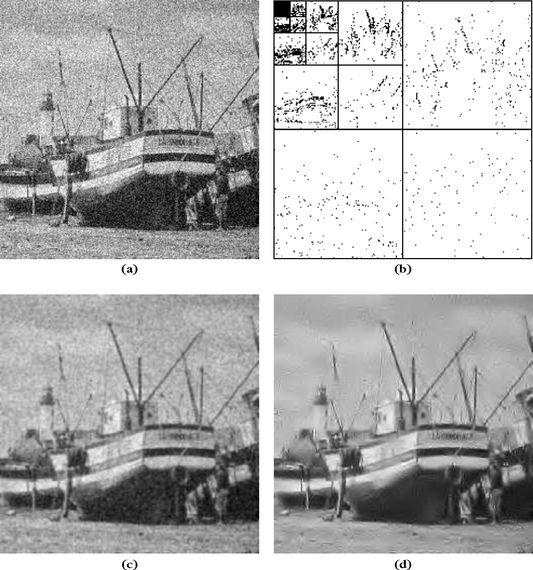
FIGURE 1.2 (a) Noisy image X. (b) Noisy wavelet coefficients above threshold, |〈X, ψj,n〈| ≥ T. (c) Linear estimation X ![]() h. (d) Nonlinear estimator recovered from thresholded wavelet coefficients over several translated bases.
h. (d) Nonlinear estimator recovered from thresholded wavelet coefficients over several translated bases.
If f has a sparse representation in a dictionary, then projecting X on the vectors of this sparse support can considerably improve linear estimators. The difficulty is identifying the sparse support of f from the noisy data X. Donoho and Johnstone [221] proved that, in an orthonormal basis, a simple thresholding of noisy coefficients does the trick. Noisy signal coefficients in an orthonormal basis B = {gm}m∈Γ are
Thresholding these noisy coefficients yields an orthogonal projection estimator
The set ![]() is an estimate of an approximation support of f. It is hopefully close to the optimal approximation support ΛT = {m ∈ Γ : |〈f, gm〉| ≥ T}.
is an estimate of an approximation support of f. It is hopefully close to the optimal approximation support ΛT = {m ∈ Γ : |〈f, gm〉| ≥ T}.
Figure 1.2(b) shows the estimated approximation set ![]() of noisy-wavelet coefficients, |〈X, ψj,n| ≥ T, that can be compared to the optimal approximation support ΛT shown in Figure 1.1(b). The estimation in Figure 1.2(d) from wavelet coefficients in
of noisy-wavelet coefficients, |〈X, ψj,n| ≥ T, that can be compared to the optimal approximation support ΛT shown in Figure 1.1(b). The estimation in Figure 1.2(d) from wavelet coefficients in ![]() has considerably reduced the noise in regular regions while keeping the sharpness of edges by preserving large-wavelet coefficients. This estimation is improved with a translation-invariant procedure that averages this estimator over several translated wavelet bases. Thresholding wavelet coefficients implements an adaptive smoothing, which averages the data X with a kernel that depends on the estimated regularity of the original signal f.
has considerably reduced the noise in regular regions while keeping the sharpness of edges by preserving large-wavelet coefficients. This estimation is improved with a translation-invariant procedure that averages this estimator over several translated wavelet bases. Thresholding wavelet coefficients implements an adaptive smoothing, which averages the data X with a kernel that depends on the estimated regularity of the original signal f.
Donoho and Johnstone proved that for Gaussian white noise of variance σ2, choosing ![]() yields a risk
yields a risk ![]() of the order of ‖f – fΛT‖2, up to a loge N factor. This spectacular result shows that the estimated support
of the order of ‖f – fΛT‖2, up to a loge N factor. This spectacular result shows that the estimated support ![]() does nearly as well as the optimal unknown support ΛT. The resulting risk is small if the representation is sparse and precise.
does nearly as well as the optimal unknown support ΛT. The resulting risk is small if the representation is sparse and precise.
The set ![]() in Figure 1.2(b) “looks” different from the ΛT in Figure 1.1(b) because it has more isolated points. This indicates that some prior information on the geometry of ΛT could be used to improve the estimation. For audio noise-reduction, thresholding estimators are applied in sparse representations provided by time-frequency bases. Similar isolated time-frequency coefficients produce a highly annoying “musical noise.” Musical noise is removed with a block thresholding that regularizes the geometry of the estimated support
in Figure 1.2(b) “looks” different from the ΛT in Figure 1.1(b) because it has more isolated points. This indicates that some prior information on the geometry of ΛT could be used to improve the estimation. For audio noise-reduction, thresholding estimators are applied in sparse representations provided by time-frequency bases. Similar isolated time-frequency coefficients produce a highly annoying “musical noise.” Musical noise is removed with a block thresholding that regularizes the geometry of the estimated support ![]() and avoids leaving isolated points. Block thresholding also improves wavelet estimators.
and avoids leaving isolated points. Block thresholding also improves wavelet estimators.
If W is a Gaussian noise and signals in Θ have a sparse representation in B, then Chapter 11 proves that thresholding estimators can produce a nearly minimax risk. In particular, wavelet thresholding estimators have a nearly minimax risk for large classes of piecewise smooth signals, including bounded variation images.
1.3 TIME-FREQUENCY DICTIONARIES
Motivated by quantum mechanics, in 1946 the physicist Gabor [267] proposed decomposing signals over dictionaries of elementary waveforms which he called time-frequency atoms that have a minimal spread in a time-frequency plane. By showing that such decompositions are closely related to our perception of sounds, and that they exhibit important structures in speech and music recordings, Gabor demonstrated the importance of localized time-frequency signal processing. Beyond sounds, large classes of signals have sparse decompositions as sums of time-frequency atoms selected from appropriate dictionaries. The key issue is to understand how to construct dictionaries with time-frequency atoms adapted to signal properties.
1.3.1 Heisenberg Uncertainty
A time-frequency dictionary ![]() is composed of waveforms of unit norm
is composed of waveforms of unit norm ![]() , which have a narrow localization in time and frequency. The time localization u of
, which have a narrow localization in time and frequency. The time localization u of ![]() and its spread around u, are defined by
and its spread around u, are defined by
Similarly, the frequency localization and spread of ![]() are defined by
are defined by
shows that 〈f, φγ〉 depends mostly on the values f(t) and ![]() , where
, where ![]() and
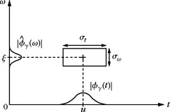
and ![]() are nonnegligible, and hence for (t, ω) in a rectangle centered at (u, ξ), of size
are nonnegligible, and hence for (t, ω) in a rectangle centered at (u, ξ), of size ![]() . This rectangle is illustrated by Figure 1.3 in this time-frequency plane (t, ω). It can be interpreted as a “quantum of information” over an elementary resolution cell. The uncertainty principle theorem proves (see Chapter 2) that this rectangle has a minimum surface that limits the joint time-frequency resolution:
. This rectangle is illustrated by Figure 1.3 in this time-frequency plane (t, ω). It can be interpreted as a “quantum of information” over an elementary resolution cell. The uncertainty principle theorem proves (see Chapter 2) that this rectangle has a minimum surface that limits the joint time-frequency resolution:
Constructing a dictionary of time-frequency atoms can thus be thought of as covering the time-frequency plane with resolution cells having a time width ![]() which may vary but with a surface larger than one-half Windowed Fourier and wavelet transforms are two important examples.
which may vary but with a surface larger than one-half Windowed Fourier and wavelet transforms are two important examples.
1.3.2 Windowed Fourier Transform
A windowed Fourier dictionary is constructed by translating in time and frequency a time window g(t), of unit norm ‖g‖ = 1, centered at t = 0:
The atom gu,ξ is translated by u in time and by ξ in frequency. The time-and-frequency spread of gu,ξ is independent of u and ξ. This means that each atom gu,ξ corresponds to a Heisenberg rectangle that has a size ![]() independent of its position (u, ξ), as shown by Figure 1.4.
independent of its position (u, ξ), as shown by Figure 1.4.
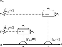
FIGURE 1.4 Time-frequency boxes (“Heisenberg rectangles”) representing the energy spread of two windowed Fourier atoms.
The windowed Fourier transform projects f on each dictionary atom gu,ξ:
It can be interpreted as a Fourier transform of f at the frequency ξ, localized by the window g(t – u) in the neighborhood of u. This windowed Fourier transform is highly redundant and represents one-dimensional signals by a time-frequency image in (u, ξ). It is thus necessary to understand how to select many fewer time-frequency coefficients that represent the signal efficiently.
When listening to music, we perceive sounds that have a frequency that varies in time. Chapter 4 shows that a spectral line of f creates high-amplitude windowed Fourier coefficients Sf(u, ξ) at frequencies ξ(u) that depend on time u. These spectral components are detected and characterized by ridge points, which are local maxima in this time-frequency plane. Ridge points define a time-frequency approximation support Λ of f with a geometry that depends on the time-frequency evolution of the signal spectral components. Modifying the sound duration or audio transpositions are implemented by modifying the geometry of the ridge support in time frequency.
A windowed Fourier transform decomposes signals over waveforms that have the same time and frequency resolution. It is thus effective as long as the signal does not include structures having different time-frequency resolutions, some being very localized in time and others very localized in frequency. Wavelets address this issue by changing the time and frequency resolution.
1.3.3 Continuous Wavelet Transform
In reflection seismology, Morlet knew that the waveforms sent underground have a duration that is too long at high frequencies to separate the returns of fine, closely spaced geophysical layers. Such waveforms are called wavelets in geophysics. Instead of emitting pulses of equal duration, he thought of sending shorter waveforms at high frequencies. These waveforms were obtained by scaling the mother wavelet, hence the name of this transform. Although Grossmann was working in theoretical physics, he recognized in Morlet’s approach some ideas that were close to his own work on coherent quantum states.
Nearly forty years after Gabor, Morlet and Grossmann reactivated a fundamental collaboration between theoretical physics and signal processing, which led to the formalization of the continuous wavelet transform [288]. These ideas were not totally new to mathematicians working in harmonic analysis, or to computer vision researchers studying multiscale image processing. It was thus only the beginning of a rapid catalysis that brought together scientists with very different backgrounds.
A wavelet dictionary is constructed from a mother wavelet ψ of zero average
which is dilated with a scale parameter s, and translated by u:
The continuous wavelet transform of f at any scale s and position u is the projection of f on the corresponding wavelet atom:
It represents one-dimensional signals by highly redundant time-scale images in (u, s).
Varying Time-Frequency Resolution
As opposed to windowed Fourier atoms, wavelets have a time-frequency resolution that changes. The wavelet ψu,s has a time support centered at u and proportional to s. Let us choose a wavelet ψ whose Fourier transform ![]() is nonzero in a positive frequency interval centered at η. The Fourier transform
is nonzero in a positive frequency interval centered at η. The Fourier transform ![]() is dilated by 1/s and thus is localized in a positive frequency interval centered at ξ = η/s; its size is scaled by 1/s. In the time-frequency plane, the Heisenberg box of a wavelet atom
is dilated by 1/s and thus is localized in a positive frequency interval centered at ξ = η/s; its size is scaled by 1/s. In the time-frequency plane, the Heisenberg box of a wavelet atom ![]() is therefore a rectangle centered at (u, η/s), with time and frequency widths, respectively, proportional to s and 1/s. When s varies, the time and frequency width of this time-frequency resolution cell changes, but its area remains constant, as illustrated by Figure 1.5.
is therefore a rectangle centered at (u, η/s), with time and frequency widths, respectively, proportional to s and 1/s. When s varies, the time and frequency width of this time-frequency resolution cell changes, but its area remains constant, as illustrated by Figure 1.5.
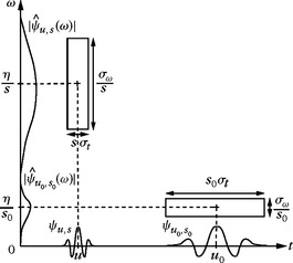
FIGURE 1.5 Heisenberg time-frequency boxes of two wavelets, ψu,s and ψu0,s0. When the scale s decreases, the time support is reduced but the frequency spread increases and covers an interval that is shifted toward high frequencies.
Large-amplitude wavelet coefficients can detect and measure short high-frequency variations because they have a narrow time localization at high frequencies. At low frequencies their time resolution is lower, but they have a better frequency resolution. This modification of time and frequency resolution is adapted to represent sounds with sharp attacks, or radar signals having a frequency that may vary quickly at high frequencies.
Multiscale Zooming
A wavelet dictionary is also adapted to analyze the scaling evolution of transients with zooming procedures across scales. Suppose now that ψ is real. Since it has a zero average, a wavelet coefficient Wf(u, s) measures the variation of f in a neighborhood of u that has a size proportional to s. Sharp signal transitions create large-amplitude wavelet coefficients.
Signal singularities have specific scaling invariance characterized by Lipschitz exponents. Chapter 6 relates the pointwise regularity of f to the asymptotic decay of the wavelet transform amplitude |Wf(u, s)| when s goes to zero. Singularities are detected by following the local maxima of the wavelet transform across scales.
In images, wavelet local maxima indicate the position of edges, which are sharp variations of image intensity. It defines scale-space approximation support of f from which precise image approximations are reconstructed. At different scales, the geometry of this local maxima support provides contours of image structures of varying sizes. This multiscale edge detection is particularly effective for pattern recognition in computer vision [146].
The zooming capability of the wavelet transform not only locates isolated singular events, but can also characterize more complex multifractal signals having nonisolated singularities. Mandelbrot [41] was the first to recognize the existence of multifractals in most corners of nature. Scaling one part of a multifractal produces a signal that is statistically similar to the whole. This self-similarity appears in the continuous wavelet transform, which modifies the analyzing scale. From global measurements of the wavelet transform decay, Chapter 6 measures the singularity distribution of multifractals. This is particularly important in analyzing their properties and testing multifractal models in physics or in financial time series.
1.3.4 Time-Frequency Orthonormal Bases
Orthonormal bases of time-frequency atoms remove all redundancy and define stable representations. A wavelet orthonormal basis is an example of the time-frequency basis obtained by scaling a wavelet ψ with dyadic scales s = 2j and translating it by 2jn, which is written ![]() . In the time-frequency plane, the Heisenberg resolution box of
. In the time-frequency plane, the Heisenberg resolution box of ![]() is a dilation by 2j and translation by 2jn of the Heisenberg box of ψ. A wavelet orthonormal is thus a subdictionary of the continuous wavelet transform dictionary, which yields a perfect tiling of the time-frequency plane illustrated in Figure 1.6.
is a dilation by 2j and translation by 2jn of the Heisenberg box of ψ. A wavelet orthonormal is thus a subdictionary of the continuous wavelet transform dictionary, which yields a perfect tiling of the time-frequency plane illustrated in Figure 1.6.

One can construct many other orthonormal bases of time-frequency atoms, corresponding to different tilings of the time-frequency plane. Wavelet packet and local cosine bases are two important examples constructed in Chapter 8, with time-frequency atoms that split the frequency and the time axis, respectively, in intervals of varying sizes.
Wavelet Packet Bases
Wavelet bases divide the frequency axis into intervals of 1 octave bandwidth. Coifman, Meyer, and Wickerhauser [182] have generalized this construction with bases that split the frequency axis in intervals of bandwidth that may be adjusted. Each frequency interval is covered by the Heisenberg time-frequency boxes of wavelet packet functions translated in time, in order to cover the whole plane, as shown by Figure 1.7.

FIGURE 1.7 A wavelet packet basis divides the frequency axis in separate intervals of varying sizes. A tiling is obtained by translating in time the wavelet packets covering each frequency interval.
As for wavelets, wavelet-packet coefficients are obtained with a filter bank of conjugate mirror filters that split the frequency axis in several frequency intervals. Different frequency segmentations correspond to different wavelet packet bases. For images, a filter bank divides the image frequency support in squares of dyadic sizes that can be adjusted.
Local Cosine Bases
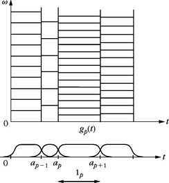
Local cosine orthonormal bases are constructed by dividing the time axis instead of the frequency axis. The time axis is segmented in successive intervals [ap, ap+1]. The local cosine bases of Malvar [368] are obtained by designing smooth windows gp(t) that cover each interval [ap, ap+1], and by multiplying them by cosine functions cos(ξt + ϕ) of different frequencies. This is yet another idea that has been independently studied in physics, signal processing, and mathematics. Malvar’s original construction was for discrete signals. At the same time, the physicist Wilson [486] was designing a local cosine basis, with smooth windows of infinite support, to analyze the properties of quantum coherent states. Malvar bases were also rediscovered and generalized by the harmonic analysts Coifman and Meyer [181]. These different views of the same bases brought to light mathematical and algorithmic properties that opened new applications.
A multiplication by cos(ξt + ϕ) translates the Fourier transform ![]() by ± ξ. Over positive frequencies, the time-frequency box of the modulated window gp(t) cos(ξt + ϕ) is therefore equal to the time-frequency box of gp translated by ξ along frequencies. Figure 1.8 shows the time-frequency tiling corresponding to such a local cosine basis. For images, a two-dimensional cosine basis is constructed by dividing the image support in squares of varying sizes.
by ± ξ. Over positive frequencies, the time-frequency box of the modulated window gp(t) cos(ξt + ϕ) is therefore equal to the time-frequency box of gp translated by ξ along frequencies. Figure 1.8 shows the time-frequency tiling corresponding to such a local cosine basis. For images, a two-dimensional cosine basis is constructed by dividing the image support in squares of varying sizes.
1.4 SPARSITY IN REDUNDANT DICTIONARIES
In natural languages, large dictionaries are needed to refine ideas with short sentences, and they evolve with usage. Eskimos have eight different words to describe snow quality, whereas a single word is typically sufficient in a Parisian dictionary. Similarly, large signal dictionaries of vectors are needed to construct sparse representations of complex signals. However, computing and optimizing a signal approximation by choosing the best M dictionary vectors is much more difficult.
1.4.1 Frame Analysis and Synthesis
Suppose that a sparse family of vectors {ϕp}p∈Λ has been selected to approximate a signal f. An approximation can be recovered as an orthogonal projection in the space VΛ generated by these vectors. We then face one of the following two problems.
1. In a dual-synthesis problem, the orthogonal projection fΛ of f in VΛ must be computed from dictionary coefficients, {〈f, ϕp〉}p∈Λ, provided by an analysis operator. This is the case when a signal transform {〈f, ϕp〉}p∈Γ is calculated in some large dictionary and a subset of inner products are selected. Such inner products may correspond to coefficients above a threshold or local maxima values.
2. In a dual-analysis problem, the decomposition coefficients of fΛ must be computed on a family of selected vectors {φp}p∈Λ. This problem appears when sparse representation algorithms select vectors as opposed to inner products. This is the case for pursuit algorithms, which compute approximation supports in highly redundant dictionaries.
The frame theory gives energy equivalence conditions to solve both problems with stable operators. A family {ϕp}p∈Λ is a frame of the space V it generates if there exists B ≥ A > 0 such that
The representation is stable since any perturbation of frame coefficients implies a modification of similar magnitude on h. Chapter 5 proves that the existence of a dual frame ![]() that solves both the dual-synthesis and dual-analysis problems:
that solves both the dual-synthesis and dual-analysis problems:
Algorithms are provided to calculate these decompositions. The dual frame is also stable:
The frame bounds A and B are redundancy factors. If the vectors {φp}p∈Γ are normalized and linearly independent, then A ≤ 1 ≤ B. Such a dictionary is called a Riesz basis of V and the dual frame is biorthogonal:
When the basis is orthonormal, then both bases are equal. Analysis and synthesis problems are then identical.
The frame theory is also used to construct redundant dictionaries that define complete, stable, and redundant signal representations, where V is then the whole signal space. The frame bounds measure the redundancy of such dictionaries. Chapter 5 studies the construction of windowed Fourier and wavelet frame dictionaries by sampling their time, frequency, and scaling parameters, while controlling frame bounds. In two dimensions, directional wavelet frames include wavelets sensitive to directional image structures such as textures or edges.
To improve the sparsity of images having edges along regular geometric curves, Candès and Donoho [134] introduced curvelet frames, with elongated waveforms having different directions, positions, and scales. Images with piecewise regular edges have representations that are asymptotically more sparse by thresholding curvelet coefficients than wavelet coefficients.
1.4.2 Ideal Dictionary Approximations
In a redundant dictionary D = {φp}p∈ Γ, we would like to find the best approximation support Λ with M = |Λ| vectors, which minimize the error ‖f – fΛ‖2. Chapter 12 proves that it is equivalent to find ΛT, which minimizes the corresponding approximation Lagrangian
Compression and denoising are two applications of redundant dictionary approximations. When compressing signals by quantizing dictionary coefficients, the distortion rate varies, like the Lagrangian (1.16), with a multiplier T that depends on the quantization step. Optimizing the coder is thus equivalent to minimizing this approximation Lagrangian. For sparse representations, most of the bits are devoted to coding the geometry of the sparse approximation set ΛT in T.
Estimators reducing noise from observations X = f + W are also optimized by finding a best orthogonal projector over a set of dictionary vectors. The model selection theory of Barron, Birgé, and Massart [97] proves that finding ![]() , which minimizes this same Lagrangian
, which minimizes this same Lagrangian ![]() , defines an estimator that has a risk on the same order as the minimum approximation error ‖f – fΛT‖2 up to a logarithmic factor. This is similar to the optimality result obtained for thresholding estimators in an orthonormal basis.
, defines an estimator that has a risk on the same order as the minimum approximation error ‖f – fΛT‖2 up to a logarithmic factor. This is similar to the optimality result obtained for thresholding estimators in an orthonormal basis.
The bad news is that minimizing the approximation Lagrangian L0 is an NP-hard problem and is therefore computationally intractable. It is necessary therefore to find algorithms that are sufficiently fast to compute suboptimal, but “good enough,” solutions.
Dictionaries of Orthonormal Bases
To reduce the complexity of optimal approximations, the search can be reduced to subfamilies of orthogonal dictionary vectors. In a dictionary of orthonormal bases, any family of orthogonal dictionary vectors can be complemented to form an orthogonal basis B included in D. As a result, the best approximation of f from orthogonal vectors in B is obtained by thresholding the coefficients of f in a “best basis” in D.
For tree dictionaries of orthonormal bases obtained by a recursive split of orthogonal vector spaces, the fast, dynamic programming algorithm of Coifman and Wickerhauser [182] finds such a best basis with O(P) operations, where P is the dictionary size.
Wavelet packet and local cosine bases are examples of tree dictionaries of time-frequency orthonormal bases of size P = N log2 N. A best basis is a time-frequency tiling that is the best match to the signal time-frequency structures.
To approximate geometrically regular edges, wavelets are not as efficient as curvelets, but wavelets provide more sparse representations of singularities that are not distributed along geometrically regular curves. Bandlet dictionaries, introduced by Le Pennec, Mallat, and Peyré [342, 365], are dictionaries of orthonormal bases that can adapt to the variability of images’ geometric regularity. Minimax optimal asymptotic rates are derived for compression and denoising.
1.4.3 Pursuit in Dictionaries
Approximating signals only from orthogonal vectors brings rigidity that limits the ability to optimize the representation. Pursuit algorithms remove this constraint with flexible procedures that search for sparse, although not necessarily optimal, dictionary approximations. Such approximations are computed by optimizing the choice of dictionary vectors {φp}p∈Λ.
Matching Pursuit
Matching pursuit algorithms introduced by Mallat and Zhang [366] are greedy algorithms that optimize approximations by selecting dictionary vectors one by one. The vector in φp0 ∈ D that best approximates a signal f is
and the residual approximation error is
A matching pursuit further approximates the residue Rf by selecting another best vector φp1 from the dictionary and continues this process over next-order residues Rmf, which produces a signal decomposition:
The approximation from the M-selected vectors {φpm}0≤m<m can be refined with an orthogonal back projection on the space generated by these vectors. An orthogonal matching pursuit further improves this decomposition by orthogonalizing progressively the projection directions φpm during the decompositon. The resulting decompositions are applied to compression, denoising, and pattern recognition of various types of signals, images, and videos.
Basis Pursuit
Approximating f with a minimum number of nonzero coefficients a[p] in a dictionary D is equivalent to minimizing the l0 norm ‖a‖0, which gives the number of nonzero coefficients. This l0 norm is highly nonconvex, which explains why the resulting minimization is NP-hard. Donoho and Chen [158] thus proposed replacing the l0 norm by the l1 norm ‖a‖1 = σp∈Γ |a[p]|, which is convex. The resulting basis pursuit algorithm computes a synthesis operator
This optimal solution is calculated with a linear programming algorithm. A basis pursuit is computationally more intense than a matching pursuit, but it is a more global optimization that yields representations that can be more sparse.
In approximation, compression, or denoising applications, f is recovered with an error bounded by a precision parameter ε. The optimization (1.18) is thus relaxed by finding a synthesis such that
This is a convex minimization problem, with a solution calculated by minimizing the corresponding l1 Lagrangian
where T is a Lagrange multiplier that depends on ε. This is called an l1 Lagrangian pursuit in this book. A solution ![]() is computed with iterative algorithms that are guaranteed to converge. The number of nonzero coordinates of
is computed with iterative algorithms that are guaranteed to converge. The number of nonzero coordinates of ![]() typically decreases as T increases.
typically decreases as T increases.
Incoherence for Support Recovery
Matching pursuit and l1 Lagrangian pursuits are optimal if they recover the approximation support ΛT, which minimizes the approximation Lagrangian
where fΛ is the orthogonal projection of f in the space VΛ generated by {φp}p∈Λ. This is not always true and depends on ΛT. An Exact Recovery Criteria proved by Tropp [464] guarantees that pursuit algorithms do recover the optimal support ΛT if
where ![]() is the biorthogonal basis of {φp}p∈ΛT in VΛT. This criterion implies that dictionary vectors φq outside ΛT should have a small inner product with vectors in ΛT.
is the biorthogonal basis of {φp}p∈ΛT in VΛT. This criterion implies that dictionary vectors φq outside ΛT should have a small inner product with vectors in ΛT.
This recovery is stable relative to noise perturbations if {φp}p∈Λ has Riesz bounds that are not too far from 1. These vectors should be nearly orthogonal and hence have small inner products. These small inner-product conditions are interpreted as a form of incoherence. A stable recovery of ΛT is possible if vectors in ΛT are incoherent with respect to other dictionary vectors and are incoherent between themselves. It depends on the geometric configuration of ΛT in Γ.
1.5 INVERSE PROBLEMS
Most digital measurement devices, such as cameras, microphones, or medical imaging systems, can be modeled as a linear transformation of an incoming analog signal, plus noise due to intrinsic measurement fluctuations or to electronic noises. This linear transformation can be decomposed into a stable analog-to-digital linear conversion followed by a discrete operator U that carries the specific transfer function of the measurement device. The resulting measured data can be written
where f ∈ ![]() N is the high-resolution signal we want to recover, and W[q] is the measurement noise. For a camera with an optic that is out of focus, the operator U is a low-pass convolution producing a blur. For a magnetic resonance imaging system, U is a Radon transform integrating the signal along rays and the number Q of measurements is smaller than N. In such problems, U is not invertible and recovering an estimate of f is an ill-posed inverse problem.
N is the high-resolution signal we want to recover, and W[q] is the measurement noise. For a camera with an optic that is out of focus, the operator U is a low-pass convolution producing a blur. For a magnetic resonance imaging system, U is a Radon transform integrating the signal along rays and the number Q of measurements is smaller than N. In such problems, U is not invertible and recovering an estimate of f is an ill-posed inverse problem.
Inverse problems are among the most difficult signal-processing problems with considerable applications. When data acquisition is difficult, costly, or dangerous, or when the signal is degraded, super-resolution is important to recover the highest possible resolution information. This applies to satellite observations, seismic exploration, medical imaging, radar, camera phones, or degraded Internet videos displayed on high-resolution screens. Separating mixed information sources from fewer measurements is yet another super-resolution problem in telecommunication or audio recognition.
Incoherence, sparsity, and geometry play a crucial role in the solution of ill-defined inverse problems. With a sensing matrix U with random coefficients, Candès and Tao [139] and Donoho [217] proved that super-resolution becomes stable for signals having a sufficiently sparse representation in a dictionary. This remarkable result opens the door to new compression sensing devices and algorithms that recover high-resolution signals from a few randomized linear measurements.
1.5.1 Diagonal Inverse Estimation
In an ill-posed inverse problem,
the image space ImU = {U h : h ∈ ![]() N} of U is of dimension Q smaller than the high-resolution space N where f belongs. Inverse problems include two difficulties. In the image space ImU, where U is invertible, its inverse may amplify the noise W, which then needs to be reduced by an efficient denoising procedure. In the null space NullU, all signals h are set to zero U h = 0 and thus disappear in the measured data Y. Recovering the projection of f in NullU requires using some strong prior information. A super-resolution estimator recovers an estimation of f in a dimension space larger than Q and hopefully equal to N, but this is not always possible.
N} of U is of dimension Q smaller than the high-resolution space N where f belongs. Inverse problems include two difficulties. In the image space ImU, where U is invertible, its inverse may amplify the noise W, which then needs to be reduced by an efficient denoising procedure. In the null space NullU, all signals h are set to zero U h = 0 and thus disappear in the measured data Y. Recovering the projection of f in NullU requires using some strong prior information. A super-resolution estimator recovers an estimation of f in a dimension space larger than Q and hopefully equal to N, but this is not always possible.
Singular Value Decompositions
Let f = σm∈Γ a[m]gm be the representation of f in an orthonormal basis B = {gm}m∈Γ. An approximation must be recovered from
A basis B of singular vectors diagonalizes U*U. Then U transforms a subset of Q vectors {gm}m∈ΓQ of B into an orthogonal basis {Ugm}m∈ΓQ of ImU and sets all other vectors to zero. A singular value decomposition estimates the coefficients a[m] of f by projecting Y on this singular basis and by renormalizing the resulting coefficients
where h2m are regularization parameters.
Such estimators recover nonzero coefficients in a space of dimension Q and thus bring no super-resolution. If U is a convolution operator, then B is the Fourier basis and a singular value estimation implements a regularized inverse convolution.
Diagonal Thresholding Estimation
The basis that diagonalizes U*U rarely provides a sparse signal representation. For example, a Fourier basis that diagonalizes convolution operators does not efficiently approximate signals including singularities.
Donoho [214] introduced more flexibility by looking for a basis B providing a sparse signal representation, where a subset of Q vectors {gm}m∈ΓQ are transformed by U in a Riesz basis {Ugm}m∈ΓQ of ImU, while the others are set to zero. With an appropriate renormalization, ![]() has a biorthogonal basis
has a biorthogonal basis ![]() that is normalized
that is normalized ![]() . The sparse coefficients of f in B can then be estimated with a thresholding
. The sparse coefficients of f in B can then be estimated with a thresholding
for thresholds Tm appropriately defined.
For classes of signals that are sparse in B, such thresholding estimators may yield a nearly minimax risk, but they provide no super-resolution since this nonlinear projector remains in a space of dimension Q. This result applies to classes of convolution operators U in wavelet or wavelet packet bases. Diagonal inverse estimators are computationally efficient and potentially optimal in cases where super-resolution is not possible.
1.5.2 Super-resolution and Compressive Sensing
Suppose that f has a sparse representation in some dictionary D = {gp}p∈Γ of P normalized vectors. The P vectors of the transformed dictionary DU = UD = {Ugp}p∈Γ belong to the space ImU of dimension Q < P and thus define a redundant dictionary. Vectors in the approximation support Λ of f are not restricted a priori to a particular subspace of ![]() N. Super-resolution is possible if the approximation support Λ of f in D can be estimated by decomposing the noisy data Y over DU. It depends on the properties of the approximation support Λ of f in Γ.
N. Super-resolution is possible if the approximation support Λ of f in D can be estimated by decomposing the noisy data Y over DU. It depends on the properties of the approximation support Λ of f in Γ.
Geometric Conditions for Super-resolution
Let wΛ = f – fΛ. be the approximation error of a sparse representation fΛ = σp∈Λ a[p]gp of f. The observed signal can be written as
If the support Λ can be identified by finding a sparse approximation of Y inDU
then we can recover a super-resolution estimation of f
This shows that super-resolution is possible if the approximation support Λ can be identified by decomposing Y in the redundant transformed dictionary DU. If the exact recovery criteria is satisfy ERC(Λ) < 1 and if {Ugp}p∈Λ is a Riesz basis, then Λ can be recovered using pursuit algorithms with controlled error bounds.
For most operator U, not all sparse approximation sets can be recovered. It is necessary to impose some further geometric conditions on Λ in Γ, which makes super-resolution difficult and often unstable. Numerical applications to sparse spike deconvolution, tomography, super-resolution zooming, and inpainting illustrate these results.
Compressive Sensing with Randomness
Candès and Tao [139], and Donoho [217] proved that stable super-resolution is possible for any sufficiently sparse signal f if U is an operator with random coefficients. Compressive sensing then becomes possible by recovering a close approximation of f ∈ ![]() N from Q
N from Q ![]() N linear measurements [133].
N linear measurements [133].
A recovery is stable for a sparse approximation set |Λ| ≤ M only if the corresponding dictionary family {Ugm}m∈Λ is a Riesz basis of the space it generates. The M-restricted isometry conditions of Candès, Tao, and Donoho [217] imposes uniform Riesz bounds for all sets Λ ⊂ Γ with |Λ| ≤ M:
This is a strong incoherence condition on the P vectors of {Ugm}m∈Γ, which supposes that any subset of less than M vectors is nearly uniformly distributed on the unit sphere of ImU.
For an orthogonal basis D = {gm}m∈Γ, this is possible for M ≤ C Q(log N)−1 if U is a matrix with independent Gaussian random coefficients. A pursuit algorithm then provides a stable approximation of any f ∈ CN having a sparse approximation from vectors in D.
These results open a new compressive-sensing approach to signal acquisition and representation. Instead of first discretizing linearly the signal at a high-resolution N and then computing a nonlinear representation over M coefficients in some dictionary, compressive-sensing measures directly M randomized linear coefficients. A reconstructed signal is then recovered by a nonlinear algorithm, producing an error that can be of the same order of magnitude as the error obtained by the more classic two-step approximation process, with a more economic acquisiton process. These results remain valid for several types of random matrices U. Examples of applications to single-pixel cameras, video super-resolution, new analog-to-digital converters, and MRI imaging are described.
Blind Source Separation
Sparsity in redundant dictionaries also provides efficient strategies to separate a family of signals {fs}0≤s<S that are linearly mixed in K ≤ S observed signals with noise:

From a stereo recording, separating the sounds of S musical instruments is an example of source separation with k = 2. Most often the mixing matrix U = {uk,s}0≤k<K,0≤s<S is unknown. Source separation is a super-resolution problem since S N data values must be recovered from Q = K N ≤ S N measurements. Not knowing the operator U makes it even more complicated.
If each source fs has a sparse approximation support Λs in a dictionary D, with Σ S–1s=0|Λs| ![]() N, then it is likely that the sets {Λs}0≤s < s are nearly disjoint. In this case, the operator U, the supports Λs, and the sources fs are approximated by computing sparse approximations of the observed data Yk in D. The distribution of these coefficients identifies the coefficients of the mixing matrix U and the nearly disjoint source supports. Time-frequency separation of sounds illustrate these results.
N, then it is likely that the sets {Λs}0≤s < s are nearly disjoint. In this case, the operator U, the supports Λs, and the sources fs are approximated by computing sparse approximations of the observed data Yk in D. The distribution of these coefficients identifies the coefficients of the mixing matrix U and the nearly disjoint source supports. Time-frequency separation of sounds illustrate these results.
1.6 TRAVEL GUIDE
1.6.1 Reproducible Computational Science
This book covers the whole spectrum from theorems on functions of continuous variables to fast discrete algorithms and their applications. Section 1.1.2 argues that models based on continuous time functions give useful asymptotic results for understanding the behavior of discrete algorithms. Still, a mathematical analysis alone is often unable to fully predict the behavior and suitability of algorithms for specific signals. Experiments are necessary and such experiments should be reproducible, just like experiments in other fields of science [124].
The reproducibility of experiments requires having complete software and full source code for inspection, modification, and application under varied parameter settings. Following this perspective, computational algorithms presented in this book are available as MATLAB subroutines or in other software packages. Figures can be reproduced and the source code is available. Software demonstrations and selected exercise solutions are available at http://wavelet-tour.com. For the instructor, solutions are available at www.elsevierdirect.com/9780123743701.
1.6.2 Book Road Map
Some redundancy is introduced between sections to avoid imposing a linear progression through the book. The preface describes several possible programs for a sparse signal-processing course.
All theorems are explained in the text and reading the proofs is not necessary to understand the results. Most of the book’s theorems are proved in detail, and important techniques are included. Exercises at the end of each chapter give examples of mathematical, algorithmic, and numeric applications, ordered by level of difficulty from 1 to 4, and selected solutions can be found at http://wavelet-tour.com.
The book begins with Chapters 2 and 3, which review the Fourier transform and linear discrete signal processing. They provide the necessary background for readers with no signal-processing background. Important properties of linear operators, projectors, and vector spaces can be found in the Appendix. Local time-frequency transforms and dictionaries are presented in Chapter 4; the wavelet and windowed Fourier transforms are introduced and compared. The measurement of instantaneous frequencies illustrates the limitations of time-frequency resolution. Dictionary stability and redundancy are introduced in Chapter 5 through the frame theory, with examples of windowed Fourier, wavelet, and curvelet frames. Chapter 6 explains the relationship between wavelet coefficient amplitude and local signal regularity. It is applied to the detection of singularities and edges and to the analysis of multifractals.
Wavelet bases and fast filter bank algorithms are important tools presented in Chapter 7. An overdose of orthonormal bases can strike the reader while studying the construction and properties of wavelet packets and local cosine bases in Chapter 8. It is thus important to read Chapter 9, which describes sparse approximations in bases. Signal-compression and denoising applications described in Chapters 10 and 11 give life to most theoretical and algorithmic results in the book. These chapters offer a practical perspective on the relevance of linear and nonlinear signal-processing algorithms. Chapter 12 introduces sparse decompositions in redundant dictionaries and their applications. The resolution of inverse problems is studied in Chapter 13, with super-resolution, compressive sensing, and source separation.