
CHAPTER 5 Frames
A signal representation may provide “analysis” coefficients that are inner products with a family of vectors, or “synthesis” coefficients that compute an approximation by recombining a family of vectors. Frames are families of vectors where “analysis” and “synthesis” representations are stable. Signal reconstructions are computed with a dual frame. Frames are potentially redundant and thus more general than bases, with a redundancy measured by frame bounds. They provide the flexibility needed to build signal representations with unstructured families of vectors.
Complete and stable wavelet and windowed Fourier transforms are constructed with frames of wavelets and windowed Fourier atoms. In two dimensions, frames of directional wavelets and curvelets are introduced to analyze and process multiscale image structures.
5.1 FRAMES AND RIESZ BASES
5.1.1 Stable Analysis and Synthesis Operators
The frame theory was originally developed by Duffin and Schaeffer [235] to reconstruct band-limited signals from irregularly spaced samples. They established general conditions to recover a vector f in a Hilbert space H from its inner products with a family of vectors {φn}n∈Γ. The index set Γ might be finite or infinite. The following frame definition gives an energy equivalence to invert the operator Φ defined by
Definition 5.1:
Frame and Riesz Basis. The sequence {φn}n∈Γ is a frame of H if there exist two constants B ≥ A > 0 such that
When A = B the frame is said to be tight. If the {φn}n∈Γ are linearly independant then the frame is not redundant and is called a Riesz basis.
If the frame condition is satisfied, then Φ is called a frame analysis operator. Section 5.1.2 proves that (5.2) is a necessary and sufficient condition guaranteeing that Φ is invertible on its image space, with a bounded inverse. Thus, a frame defines a complete and stable signal representation, which may also be redundant.
Frame Synthesis
Let us consider the space of finite energy coefficients
The adjoint Φ* of Φ is defined over ![]() 2(Γ) and satisfies for any f ∈ H and a ∈
2(Γ) and satisfies for any f ∈ H and a ∈ ![]() 2(Γ):
2(Γ):
It is therefore the synthesis operator
The frame condition (5.2) can be rewritten as
It results that A and B are the infimum and supremum values of the spectrum of the symmetric operator Φ*Φ, which correspond to the smallest and largest eigenvalues in finite dimension. The eigenvalues are also called singular values of Φ or singular spectrum. Theorem 5.1 derives that the frame synthesis operator is also stable.
Theorem 5.1.
The family {φn}n∈Γ is a frame with bounds 0 < A ≤ B if and only if
Proof.
Since Φ*a = Σn∈Γ a[n] φn, it results that
The operator Φ is a frame if and only if the spectrum of Φ*Φ is bound by A and B. The inequality (5.5) states that the spectrum of Φ Φ* over ImΦ is also bounded by A and B. Both statements are proved to be equivalent by verifying that the supremum and infimum of the spectrum of Φ*Φ are equal to the supremum and infimum of the spectrum of Φ*Φ.
In finite dimension, if λ is an eigenvalue of Φ*Φ with eigenvector f, then λ is also an eigenvalue of Φ*Φ with eigenvector Φf. Indeed, Φ*Φf = λf so Φ Φ*(Φf) =λΦf and Φf ≠ 0, because the left frame inequality (5.2) implies that ‖Φf‖2 ≤ A ‖f‖2. It results that the maximum and minimum eigenvectors of Φ*Φ and Φ Φ* on ImΦ are identical.
In a Hilbert space of infinite dimension, we prove that the supremum and infimum of the spectrum of both operators remain identical by growing the space dimension, and computing the limit of the largest and smallest eigenvalues when the space dimension tends to infinity.
This theorem proves that linear combination of frame vectors define a stable signal representation. Section 5.1.2 proves that synthesis coefficients are computed with a dual frame. The operator Φ Φ* is the Gram matrix {〈φn, φp〉}(m,p)∈![]() 2(Γ):
2(Γ):
One must be careful because (5.5) is only valid for a ∈ ImΦ. If it is valid for all a ∈ ![]() 2 (Γ) with A > 0 then the family is linearly independant and is thus a Riesz basis.
2 (Γ) with A > 0 then the family is linearly independant and is thus a Riesz basis.
Redundancy
When the frame vectors are normalized ‖φn‖ = 1, Theorem 5.2 shows that the frame redundancy is measured by the frame bounds A and B.
Theorem 5.2.
In a space of finite dimension N, a frame of P ≥ N normalized vectors has frame bounds A and B, which satisfy
For a tight frame A = B = P/N.
Proof.
It results from (5.4) that all eigenvalues of Φ*Φ are between A and B. The trace of Φ*Φ thus satisfies
But since the trace is not modified by commuting matrices (Exercise 5.4), and ‖φn‖ = 1,
which implies (5.7).
If {φn}n∈Γ is a normalized Riesz basis and is therefore linearly independent, then (5.7) proves that A ≤ 1 ≤ B. This result remains valid in infinite dimension. Inserting f = φn in the frame inequality (5.2) proves that the frame is orthonormal if and only if B = 1, in which case A = 1.
One can verify (Exercise 5.3) that a finite set of N vectors {φn}1≤n≤N is always a frame of the space V generated by linear combinations of these vectors. When N increases, the frame bounds A and B may go respectively to 0 and +∞. This illustrates the fact that in infinite dimensional spaces, a family of vectors may be complete and not yield a stable signal representation.
Irregular Sampling
Let Us be the space of L2(![]() ) functions having a Fourier transform support included in [−π/s, π/s]. For a uniform sampling, tn = ns, Theorem 3.5 proves that if φs(t) = s1/2 sin(π/s−1 t)/(πt), then {φs(t − ns)}n∈
) functions having a Fourier transform support included in [−π/s, π/s]. For a uniform sampling, tn = ns, Theorem 3.5 proves that if φs(t) = s1/2 sin(π/s−1 t)/(πt), then {φs(t − ns)}n∈![]() is an orthonormal basis of Us. The reconstruction of f from its samples is then given by the sampling Theorem 3.2.
is an orthonormal basis of Us. The reconstruction of f from its samples is then given by the sampling Theorem 3.2.
The irregular sampling conditions of Duffin and Schaeffer [235] for constructing a frame were later refined by several researchers [81, 102, 500]. Gröchenig proved [285] that if ![]() and
and ![]() , and if the maximum sampling distance δ satisfies
, and if the maximum sampling distance δ satisfies
is a frame with frame bounds A ≥ (1 – δ/s)2 and B ≤ (1 + δ/s)2. The amplitude factor λn compensates for the increase of sample density relatively to s. The reconstruction of f requires inverting the frame operator Φf[n] = 〈f(u), λn, φs(u – tn)〉.
5.1.2 Dual Frame and Pseudo Inverse
The reconstruction of f from its frame coefficients Φf[n] is calculated with a pseudo inverse also called Moore-Penrose pseudo inverse. This pseudo inverse is a bounded operator that implements a dual-frame reconstruction. For Riesz bases, this dual frame is a biorthogonal basis.
For any operator U, we denote by ImU the image space of all U f and by NullU the null space of all h, such that Uh = 0.
Theorem 5.3.
If {φn}n∈Γ is a frame but not a Riesz basis, then Φ admits an infinite number of left inverses.
Proof.
We know that NullΦ* = (ImΦ)⊥ is the orthogonal complement of ImΦ in ![]() 2(Γ) (Exercise 5.7). If Φ is a frame and not a Riesz basis, then {φn}n∈Γ is linearly dependent, so there exists a ∈ NullΦ* = (ImΦ)⊥ with a ≠ 0.
2(Γ) (Exercise 5.7). If Φ is a frame and not a Riesz basis, then {φn}n∈Γ is linearly dependent, so there exists a ∈ NullΦ* = (ImΦ)⊥ with a ≠ 0.
A frame operator Φ is injective (one to one). Indeed, the frame inequality (5.2) guarantees that Φf = 0 implies f = 0. Its restriction to ImΦ is thus invertible, which means that Φ admits a left inverse. There is an infinite number of left inverses since the restriction of a left inverse to (ImΦ)⊥ ≠ {0} may be any arbitrary linear operator.
The more redundant the frame {φn}n∈Γ, the larger the orthogonal complement (ImΦ)⊥ of ImΦ in ![]() 2(Γ). The pseudo inverse, written as Φ+, is defined as the left inverse that is zero on (ImΦ)⊥:
2(Γ). The pseudo inverse, written as Φ+, is defined as the left inverse that is zero on (ImΦ)⊥:
Theorem 5.4 computes this pseudo inverse.
Theorem 5.4:
Pseudo Inverse. If Φ is a frame operator, then Φ*Φ is invertible and the pseudo inverse satisfies
Proof.
The frame condition in (5.4) is rewritten as
The result is that Φ*Φ is an injective self-adjoint operator: Φ*Φ f = 0 if and only if f = 0. It is therefore invertible. For all f ∈ H,
so Φ+ is a left inverse. Since (ImΦ)⊥ = NullΦ*, it results that Φ+ a = 0 for any a ∈ (ImΦ)⊥ = NullΦ*. Since this left inverse vanishes on (ImΦ)⊥, it is the pseudo inverse.
Dual Frame
The pseudo inverse of a frame operator implements a reconstruction with a dual frame, which is specified by Theorem 5.5.
Theorem 5.5.
Let {φn}n∈Γ be a frame with bounds 0 < A ≤ B. The dual operator defined by
If the frame is tight (i.e., A = B),![]() then
then
Proof.
The dual operator can be written as ![]() . Indeed,
. Indeed,
Thus, we derive from (5.10) that its adjoint is the pseudo inverse of Φ:
It results that ![]() and thus that
and thus that ![]() , which proves (5.12).
, which proves (5.12).
Let us now prove the frame bounds (5.13). Frame conditions are rewritten in (5.4):
Lemma 5.1 applied to L = Φ*Φ proves that
the dual-frame bounds (5.13) are derived from (5.15).
If A = B, then 〈Φ*Φf, f〉 = A ‖f‖2. Thus, the spectrum of Φ*Φ is reduced to A and therefore Φ*Φ = A Id. As a result, φn = (Φ*Φ)−1 φn = A−1 φn.
Lemma 5.1.
If L is a self-adjoint operator such that there exist B ≥ A > 0 satisfying
In finite dimensions, since L is self-adjoint we know that it is diagonalized in an orthonormal basis. The inequality (5.16) proves that its eigenvalues are between A and B. It is therefore invertible with eigenvalues between B−1 and A−1, which proves (5.17). In a Hilbert space of infinite dimension, we prove that same result on the supremum and infimum of the spectrum by growing the space dimension, and computing the limit of the largest and smallest eigenvalues when the space dimension tends to infinity.
This theorem proves that f is reconstructed from frame coefficients Φf[n] = 〈f, φn〉 with the dual frame {φn}n∈Γ. The synthesis coefficients of f in {φn}n∈Γ are the dual-frame coefficients Φf[n] = 〈f, φn〉. If the frame is tight, then both decompositions are identical:
Biorthogonal Bases
A Riesz basis is a frame of vectors that are linearly independent, which implies that ImΦ = ![]() 2(Γ), so its dual frame is also linearly independent. Inserting f = φp in (5.12) yields
2(Γ), so its dual frame is also linearly independent. Inserting f = φp in (5.12) yields
and the linear independence implies that
Thus, dual Riesz bases are biorthogonal families of vectors. If the basis is normalized (i.e., ‖φn‖ = 1), then
This is proved by inserting f = φp in the frame inequality (5.13):
5.1.3 Dual-Frame Analysis and Synthesis Computations
Suppose that {φn}n∈Γ is a frame of a subspace V of the whole signal space. The best linear approximation of f in V is the orthogonal projection of f in V. Theorem 5.6 shows that this orthogonal projection is computed with the dual frame. Two iterative numerical algorithms are described to implement such computations.
Theorem 5.6.
Let {φn}n∈Γ be a frame of V, and ![]() it’s dual frame in V. The orthogonal projection of f ∈ H in V is
it’s dual frame in V. The orthogonal projection of f ∈ H in V is
Proof.
Since both frames are dual in V, if f ∈ V, then, (5.12) proves that the operator PV defined in (5.20) satisfies PV f = f. To prove that it is an orthogonal projection it is sufficient to verify that if f ∈ H then 〈f − PV f, φp〉 = 0 for all p ∈ Γ. Indeed,
because the dual-frame property implies that ![]() .
.
If Γ is finite, then {φn}n∈Γ is necessarily a frame of the space V it generates, and (5.20) reconstructs the best linear approximation of f in V. This result is particularly important for approximating signals from a finite set of vectors.
Since Φ is not a frame of the whole signal space H, but of a subspace V then Φ is only invertible on this subspace and the pseudo-inverse definition becomes:
Let ΦV be the restriction of Φ to V. The operator Φ*ΦV is invertible on V and we write (Φ*ΦV)−1 its inverse. Similar to (5.10), we verify that Φ+ = (Φ*ΦV)−1 Φ*.
Dual Synthesis
In a dual synthesis problem, the orthogonal projection is computed from the frame coefficients {Φf[n] = 〈f, φn〉}n∈T with the dual-frame synthesis operator:
If the frame {φn}n∈Γ does not depend on the signal f, then the dual-frame vectors are precomputed with (5.11):
and the dual synthesis is solved directly with (5.22). In many applications, the frame vectors {φn}n∈Γ depend on the signal f, in which case the dual-frame vectors ![]() cannot be computed in advance, and it is highly inefficient to compute them. This is the case when coefficients {〈f, φn〉}n∈Γ are selected in a redundant transform, to build a sparse signal representation. For example, the time-frequency ridge vectors in Sections 4.4.2 and 4.4.3 are selected from the local maxima of f in highly redundant windowed Fourier or wavelet transforms.
cannot be computed in advance, and it is highly inefficient to compute them. This is the case when coefficients {〈f, φn〉}n∈Γ are selected in a redundant transform, to build a sparse signal representation. For example, the time-frequency ridge vectors in Sections 4.4.2 and 4.4.3 are selected from the local maxima of f in highly redundant windowed Fourier or wavelet transforms.
The transform coefficients Φf are known and we must compute
A dual-synthesis algorithm computes first
and then derives PV f = L−1 y = z by applying the inverse of the symmetric operator L = Φ*ΦV to y, with
Dual Analysis
In a dual analysis, the orthogonal projection PVf is computed from the frame vectors {φn}n∈Γ with the dual-frame analysis operator ![]() :
:
If {φn}n∈Γ does not depend upon f then ![]() is precomputed with (5.23). The {φn}n∈Γ may also be selected adaptively from a larger dictionary, to provide a sparse approximation of f. Computing the orthogonal projection PVf is called a backprojection. In Section 12.3, matching pursuits implement this backprojection.
is precomputed with (5.23). The {φn}n∈Γ may also be selected adaptively from a larger dictionary, to provide a sparse approximation of f. Computing the orthogonal projection PVf is called a backprojection. In Section 12.3, matching pursuits implement this backprojection.
When {φn}n∈Γ depends on f, computing the dual frame is inefficient. The dual coefficient ![]() is calculated directly, as well as
is calculated directly, as well as
Since ΦPV f = Φf, we have Φ Φ*a = Φf. Let Φ*ImΦ be the restriction of Φ* to ImΦ. Since Φ Φ*ImΦ is invertible on ImΦ
Thus, the dual-analysis algorithm computes y = Φf = {〈f, φn〉}n∈Γ and derives the dual coefficients a = L−1 y = z by applying the inverse of the Gram operator L = Φ Φ*ImΦ to y, with
The eigenvalues of L are also between A and B. The orthogonal projection of f is recovered with (5.26).
Richardson Inversion of Symmetric Operators
The key computational step of a dual-analysis or a dual-synthesis problem is to compute z = L−1y, where L is a symmetric operator with eigenvalues that are between A and B. Theorems 5.7 and 5.8 describe two iterative algorithms with exponential convergence. The Richardson iteration procedure is simpler but requires knowing the frame bounds A and B. Conjugate gradient iterations converge more quickly when B/A is large, and do not require knowing the values of A and B.
Theorem 5.7.
To compute z = L−1y, let z0 be an initial value and γ > 0 be a relaxation parameter. For any k > 0, define
Proof.
The induction equation (5.28) can be rewritten as
Since the eigenvalues of L are between A and B,
This implies that R = I − γL satisfies
where δ is given by (5.29). Since R is symmetric, this inequality proves that ‖R‖ ≤ δ. Thus, we derive (5.30) from (5.31). The error ‖z − zk‖ clearly converges to zero if δ < 1.
The convergence is guaranteed for all initial values z0. If an estimation z0 of the solution z is known, then this estimation can be chosen; otherwise, z0 is often set to 0. For frame inversion, the Richardson iteration algorithm is sometimes called the frame algorithm [19]. The convergence rate is maximized when δ is minimum:
which corresponds to the relaxation parameter
The algorithm converges quickly if A/B is close to 1. If A/B is small then
The inequality (5.30) proves that we obtain an error smaller than ε for a number n of iterations, which satisfies
Inserting (5.33) gives
Therefore, the number of iterations increases proportionally to the frame-bound ratio B/A.
The exact values of A and B are often not known, and A is generally more difficult to compute. The upper frame bound is B = ‖Φ Φ*‖s = ‖Φ* Φ‖s. If we choose
then (5.29) shows that the algorithm is guaranteed to converge, but the convergence rate depends on A. Since 0 < A ≤ B, the optimal relaxation parameter γ in (5.32) is in the range ‖Φ Φ*‖−1s ≤ γ < 2 ‖Φ Φ*‖−1S.
Conjugate-Gradient Inversion
The conjugate-gradient algorithm computes z = L−1 y with a gradient descent along orthogonal directions with respect to the norm induced by the symmetric operator L:
This L norm is used to estimate the error. Gröchenig’s [287] implementation of the conjugate-gradient algorithm is given by Theorem 5.8.
Theorem 5.8.
Conjugate Gradient. To compute z = L−1y, we initialize
For any k ≥ 0, we define by induction:
Proof.
We give the main steps of the proof as outlined by Gröchenig [287].
Step 1. Let Uk be the subspace generated by {Ljz}1≤j≤k. By induction on k, we derive from (5.41) that pj ∈ Uk, for j < k.
Step 2. We prove by induction that {pj}0≤j≤k is an orthogonal basis of Uk with respect to the inner product 〈z, h〉L = 〈z, Lh〉. Assuming that 〈pk, Lpj〉 = 0, for j ≤ k − 1, it can be shown that 〈pk + 1, Lpj〉 = 0, for j ≤ k.
Step 3. We verify that zk is the orthogonal projection of z onto Uk with respect to 〈., .〉L, which means that
Since zk ∈ Uk, this requires proving that 〈z − zk, pj〉L = 0, for j < k.
Step 4. We compute the orthogonal projection of z in embedded spaces Uk of dimension k, and one can verify that limk→ +∞ ‖z − zk‖L = 0. The exponential convergence (5.42) is proved in [287].
As opposed to the Richardson algorithm, the initial value z0 must be set to 0. As in the Richardson iteration algorithm, the convergence is slower when A/B is small. In this case,
The upper bound (5.42) proves that we obtain a relative error
Comparing this result with (5.34) shows that when A/B is small, the conjugate-gradient algorithm needs much less iterations than the Richardson iteration algorithm to compute z = L−1y at a fixed precision.
5.1.4 Frame Projector and Reproducing Kernel
Frame redundancy is useful in reducing noise added to the frame coefficients. The vector computed with noisy frame coefficients is projected on the image of Φ to reduce the amplitude of the noise. This technique is used for high-precision analog-to-digital conversion based on oversampling. The following theorem specifies the orthogonal projector on ImΦ.
Theorem 5.9.
Reproducing Kernel. Let {φn}n∈Γ be a frame of H or of a subspace V. The orthogonal projection from ![]() 2(Γ) onto ImΦ is
2(Γ) onto ImΦ is
Coefficients a ∈ e2(Γ) are frame coefficients a ∈ ImΦ if and only if they satisfy the reproducing kernel equation
Proof.
If a ∈ (ImΦ)⊥, then Pa = 0 because Φ+ a = 0. This proves that P is an orthogonal projector on ImΦ. Since Φf[n] = 〈f, φn〉 and ![]() , we derive (5.43).
, we derive (5.43).
A vector a ∈ ![]() 2(Γ) belongs to ImΦ if and only if a = Pa, which proves (5.44).
2(Γ) belongs to ImΦ if and only if a = Pa, which proves (5.44).
The reproducing kernel equation (5.44) expresses the redundancy of frame coefficients. If the frame is not redundant and is a Riesz basis, then ![]() , so this equation vanishes.
, so this equation vanishes.
Noise Reduction
Suppose that each frame coefficient Φf[n] is contaminated by an additive noise W[n], which is a random variable. Applying the projector P gives
Since P is an orthogonal projector, ‖PW‖ ≤ ‖W‖. This projector removes the component of W that is in (ImΦ)⊥. Increasing the redundancy of the frame reduces the size of ImΦ and thus increases (ImΦ)⊥, so a larger portion of the noise is removed. If W is a white noise, its energy is uniformly distributed in the space ![]() 2(Γ). Theorem 5.10 proves that its energy is reduced by at least A if the frame vectors are normalized.
2(Γ). Theorem 5.10 proves that its energy is reduced by at least A if the frame vectors are normalized.

Oversampling
This noise-reduction strategy is used by high-precision analog-to-digital converters. After a low-pass filter, a band-limited analog signal f(t) is uniformly sampled and quantized. In hardware, it is often easier to increase the sampling rate rather than the quantization precision. Increasing the sampling rate introduces a redundancy between the sample values of the band-limited signal. Thus, these samples can be interpreted as frame coefficients. For a wide range of signals it has been shown that the quantization error is nearly a white noise [277]. Thus, it can be significantly reduced by a frame projector, which in this case is a low-pass convolution operator (Exercise 5.16).
The noise can be further reduced if it is not white and if its energy is better concentrated in (ImΦ)⊥. This can be done by transforming the quantization noise into a noise that has energy mostly concentrated at high frequencies. Sigma-delta modulators produce such quantization noises by integrating the signal before its quantization [89]. To compensate for the integration, the quantized signal is differentiated. This differentiation increases the energy of the quantized noise at high frequencies and reduces its energy at low frequencies [456].
5.1.5 Translation-Invariant Frames
Section 4.1 introduces translation-invariant dictionaries obtained by translating a family of generators {φn}n∈Γ, which are used to construct translation-invariant signal representations. In multiple dimensions for φn∈L2(![]() d), the resulting dictionary can be written D = {φu,n(x)}n∈Γ, u∈
d), the resulting dictionary can be written D = {φu,n(x)}n∈Γ, u∈![]() d, with φu,n(x) = λu,n φn(x − u). In a translation-invariant wavelet dictionary, the generators are obtained by dilating a wavelet ψ(t) with scales sn: φn(t) = s−1/2n ψ(x/sn). In a window Fourier dictionary the generators are obtained by modulating a window g(x) at frequencies
d, with φu,n(x) = λu,n φn(x − u). In a translation-invariant wavelet dictionary, the generators are obtained by dilating a wavelet ψ(t) with scales sn: φn(t) = s−1/2n ψ(x/sn). In a window Fourier dictionary the generators are obtained by modulating a window g(x) at frequencies ![]()
The decomposition coefficients of f in D are convolution products
Suppose that Γ is a countable set. The overall index set ![]() d × Γ is not countable, so the dictionary D cannot strictly speaking be considered as a frame. However, if we consider the overall energy of dictionary coefficients, calculated with a sum and a multidimensional integral
d × Γ is not countable, so the dictionary D cannot strictly speaking be considered as a frame. However, if we consider the overall energy of dictionary coefficients, calculated with a sum and a multidimensional integral
and if there exist two constants A > 0 and B > 0 such that for all f ∈ L2 (![]() ),
),
then the frame theory results of the previous section apply. Thus, with an abuse of language, such translation-invariant dictionaries will also be called frames. Theorem 5.11 proves that the frame condition (5.47) is equivalent to a condition on the Fourier transform ![]() of the generators.
of the generators.
Theorem 5.11.
If there exist two constants B ≥ A > 0 such that for almost all ω in ![]() d
d
then the frame inequality (5.47) is valid for all f ∈ L2(![]() d). Any
d). Any ![]() that satisfies for almost all Ω in
that satisfies for almost all Ω in ![]() d
d
The pseudo inverse (dual frame) is implemented by
Proof.
The frame condition (5.47) means that Φ*Φ has a spectrum bounded by A and B. It results from (5.46) that
The spectrum of this convolution operator is given by the Fourier transform of ![]() , which is
, which is ![]() . Thus, the frame inequality (5.47) is equivalent to condition’ (5.48).
. Thus, the frame inequality (5.47) is equivalent to condition’ (5.48).
Equation (5.50) is proved by taking the Fourier transform on both sides and inserting (5.49).
Theorem 5.5 proves that the dual-frame vectors implementing the pseudo inverse are ![]() . Since Φ*Φ is the convolution operator (5.52), its inverse is calculated by inverting its transfer function, which yields (5.51).
. Since Φ*Φ is the convolution operator (5.52), its inverse is calculated by inverting its transfer function, which yields (5.51).
For wavelet or windowed Fourier translation-invariant dictionaries, the theorem condition (5.48) becomes a condition on the Fourier transform of the wavelet ![]() or on the Fourier transform of the window ĝ(ω). As explained in Sections 5.3 and 5.4, more conditions are needed to obtain a frame by discretizing the translation parameter u.
or on the Fourier transform of the window ĝ(ω). As explained in Sections 5.3 and 5.4, more conditions are needed to obtain a frame by discretizing the translation parameter u.
Discrete Translation-Invariant Frames
For finite-dimensional signals f[n] ∈ ![]() N a circular translation-invariant frame is obtained with a periodic shift modulo N of a finite number of generators
N a circular translation-invariant frame is obtained with a periodic shift modulo N of a finite number of generators
Such translation-invariant frames appear in Section 11.2.3 to define translation-invariant thresholding estimators for noise removal. Similar to Theorem 5.11, Theorem 5.12 gives a necessary and sufficient condition on the discrete Fourier transform ![]() of the generators φm[n] to obtain a frame.
of the generators φm[n] to obtain a frame.
Theorem 5.12.
A circular translation-invariant dictionary ![]() is a frame with frame bounds 0 < A ≤ B if and only if
is a frame with frame bounds 0 < A ≤ B if and only if
The proof proceeds essentially like the proof of Theorem 5.11, and is left in Exercise 5.8.
5.2 TRANSLATION-INVARIANT DYADIC WAVELET TRANSFORM
The continuous wavelet transform of Section 4.3 decomposes one-dimensional signals f ∈ L2 (![]() ) over a dictionary of translated and dilated wavelets
) over a dictionary of translated and dilated wavelets
Translation-invariant wavelet dictionaries are constructed by sampling the scale parameter s along an exponential sequence {vj}j∈![]() , while keeping all translation parameters u. We choose v = 2 to simplify computer implementations:
, while keeping all translation parameters u. We choose v = 2 to simplify computer implementations:
The resulting dyadic wavelet transform of f ∈ L2 (![]() ) is defined by
) is defined by
Translation-invariant dyadic wavelet transforms are used in pattern-recognition applications and for denoising with translation-invariant wavelet thresholding estimators, as explained in Section 11.3.1. Fast computations with filter banks are presented in the next two sections.
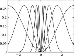
Theorem 5.11 on translation-invariant dictionaries can be applied to the multiscale wavelet generators φn(t) = 2−j/2 ψ2j(t). Since ![]() , the Fourier condition (5.48) means that there exist two constants A > 0 and B > 0 such that
, the Fourier condition (5.48) means that there exist two constants A > 0 and B > 0 such that
and since Φ f(u, n) = 2−j/2 W f(u, n), Theorem 5.11 proves the frame inequality
This shows that if the frequency axis is completely covered by dilated dyadic wavelets, as shown in Figure 5.1, then a dyadic wavelet transform defines a complete and stable representation.
then (5.50) applied to ![]() proves that
proves that
Figure 5.2 gives a dyadic wavelet transform computed over five scales with the quadratic spline wavelet shown later in Figure 5.3.
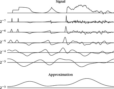
FIGURE 5.2 Dyadic wavelet transform W f(u, 2j) computed at scales 2−7 ≤ 2j ≤ 2−3 with filter bank algorithm from Section 5.2.2, for a signal defined over [0, 1]. The bottom curve carries lower frequencies corresponding to scales larger than 2−3
5.2.1 Dyadic Wavelet Design
A discrete dyadic wavelet transform can be computed with a fast filter bank algorithm if the wavelet is appropriately designed. The synthesis of these dyadic wavelets is similar to the construction of biorthogonal wavelet bases, explained in Section 7.4. All technical issues related to the convergence of infinite cascades of filters are avoided in this section. Reading Chapter 7 first is necessary for understanding the main results.
Let h and g be a pair of finite impulse-response filters. Suppose that h is a low-pass filter with a transfer function that satisfies ĥ(0) = √2. As in the case of orthogonal and biorthogonal wavelet bases, we construct a scaling function with a Fourier transform:
We suppose here that this Fourier transform is a finite-energy function so that φ ∈ L2 (![]() ). The corresponding wavelet ψ has a Fourier transform defined by
). The corresponding wavelet ψ has a Fourier transform defined by
Theorem 7.5 proves that both φ and ψ have a compact support because h and g have a finite number of nonzero coefficients. The number of vanishing moments of ψ is equal to the number of zeroes of ![]() , (5.60) implies that it is also equal to the number of zeros of ĝ(ω) at ω = 0.
, (5.60) implies that it is also equal to the number of zeros of ĝ(ω) at ω = 0.
Reconstructing Wavelets
Reconstructing wavelets that satisfy (5.49) are calculated with a pair of finite impulse response dual filters ĥ and ĝ. We suppose that the following Fourier transform has a finite energy:
 (5.61)
Theorem 5.13 gives a sufficient condition to guarantee that ![]() is the Fourier transform of a reconstruction wavelet.
is the Fourier transform of a reconstruction wavelet.
Theorem 5.13.
Proof.
The Fourier transform expressions (5.60) and (5.62) prove that
Equation (5.63) implies


Since ĝ(0) = 0, (5.63) implies ![]() . We also impose that ĥ(0) = √2, so one can derive from (5.59) and (5.61) that
. We also impose that ĥ(0) = √2, so one can derive from (5.59) and (5.61) that ![]() . Since φ and
. Since φ and ![]() belong to L1(
belong to L1(![]() ),
), ![]() and
and ![]() are continuous, and the Riemann-Lebesgue lemma (Exercise 2.8) proves that
are continuous, and the Riemann-Lebesgue lemma (Exercise 2.8) proves that ![]() and
and ![]() decrease to zero when ω goes to ∞. For ω ≠ 0, letting k and l go to +∞ yields (5.64).
decrease to zero when ω goes to ∞. For ω ≠ 0, letting k and l go to +∞ yields (5.64).
Observe that (5.63) is the same as the unit gain condition (7.117) for biorthogonal wavelets. The aliasing cancellation condition (7.116) of biorthogonal wavelets is not required because the wavelet transform is not sampled in time.
Finite Impulse Response Solution
Let us shift h and g to obtain causal filters. The resulting transfer functions ĥ(ω) and ĝ(ω) are polynomials in e−i ω. We suppose that these polynomials have no common zeros. The Bezout theorem (7.8) on polynomials proves that if P(z) and Q(z) are two polynomials of degree n and l, with no common zeros, then there exists a unique pair of polynomials ![]() and
and ![]() of degree l − 1 and n − 1 such that
of degree l − 1 and n − 1 such that
This guarantees the existence of ![]() and
and ![]() , which are polynomials in e−i ω and satisfy (5.63). These are the Fourier transforms of the finite impulse response filters
, which are polynomials in e−i ω and satisfy (5.63). These are the Fourier transforms of the finite impulse response filters ![]() and
and ![]() . However, one must be careful, because the resulting scaling function
. However, one must be careful, because the resulting scaling function ![]() in (5.61) does not necessarily have a finite energy.
in (5.61) does not necessarily have a finite energy.
Spline Dyadic Wavelets
A box spline of degree m is a translation of m + 1 convolutions of 1[0, 1] with itself. It is centered at t = 1/2 if m is even and at t = 0 if m is odd. Its Fourier transform is
We construct a wavelet that has one vanishing moment by choosing ĝ(ω) = O(ω) in the neighborhood of Ω = 0. For example,
The Fourier transform of the resulting wavelet is
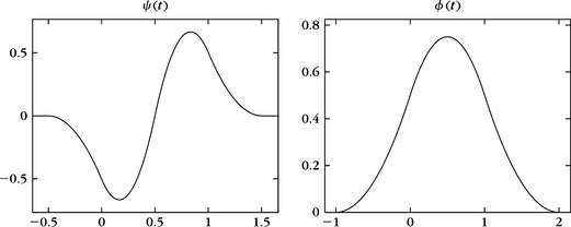
It is the first derivative of a box spline of degree m + 1 centered at t = (1 + ε)/4. For m = 2, Figure 5.3 shows the resulting quadratic splines φ and ϕ. The dyadic admissibility condition (5.48) is verified numerically for A = 0.505 and B = 0.522.
To design dual-scaling functions ![]() and wavelets
and wavelets ![]() that are splines, we choose
that are splines, we choose ![]() As a consequence,
As a consequence, ![]() and the reconstruction condition (5.63) imply that
and the reconstruction condition (5.63) imply that
Table 5.1 gives the corresponding filters for m = 2.

5.2.2 Algorithme à Trous
Suppose that the scaling functions and wavelets φ, ψ, ![]() , and
, and ![]() are designed with the filters h, g
are designed with the filters h, g ![]() , and
, and ![]() . A fast dyadic wavelet transform is calculated with a filter bank algorithm, called algorithme à trous, introduced by Holschneider et al. [303]. It is similar to a fast biorthogonal wavelet transform, without subsampling [367, 433].
. A fast dyadic wavelet transform is calculated with a filter bank algorithm, called algorithme à trous, introduced by Holschneider et al. [303]. It is similar to a fast biorthogonal wavelet transform, without subsampling [367, 433].
Fast Dyadic Transform
The samples a0[n] of the input discrete signal are written as a low-pass filtering with φ of an analog signal f, in the neighborhood of t = n:
This is further justified in Section 7.3.1. For any j ≥ 0, we denote
The dyadic wavelet coefficients are computed for j > 0 over the integer grid
For any filter x[n], we denote by xj[n] the filters obtained by inserting 2f − 1 zeros between each sample of x[n]. Its Fourier transform is ![]() . Inserting zeros in the filters creates holes (trous in French). Let
. Inserting zeros in the filters creates holes (trous in French). Let ![]() . Theorem 5.14 gives convolution formulas that are cascaded to compute a dyadic wavelet transform and its inverse.
. Theorem 5.14 gives convolution formulas that are cascaded to compute a dyadic wavelet transform and its inverse.
Theorem 5.14.
Proof of (5.71).
we verify with (3.3) that their Fourier transforms are, respectively,
The properties (5.61) and (5.62) imply that

Since j ≥ 0, both ĥ(2j ω) and ĝ(2j ω) are 2π periodic, so
These two equations are the Fourier transforms of (5.71).
Proof of (5.72).
Equation (5.73) implies

Inserting the reconstruction condition (5.63) proves that
which is the Fourier transform of (5.72).
The dyadic wavelet representation of a0 is defined as the set of wavelet coefficients up to a scale 2J plus the remaining low-frequency information aJ:
It is computed from a0 by cascading the convolutions (5.71) for 0 ≤ j < J, as illustrated in Figure 5.4(a). The dyadic wavelet transform of Figure 5.2 is calculated with the filter bank algorithm. The original signal a0 is recovered from its wavelet representation (5.74) by iterating (5.72) for J > j ≥ 0, as illustrated in Figure 5.4(b).

FIGURE 5.4 (a) The dyadic wavelet coefficients are computed by cascading convolutions with dilated filters ![]() and
and ![]() . (b) The original signal is reconstructed through convolutions with
. (b) The original signal is reconstructed through convolutions with ![]() and
and ![]() . A multiplication by 1/2 is necessary to recover the next finer scale signal aj.
. A multiplication by 1/2 is necessary to recover the next finer scale signal aj.
If the input signal a0[n] has a finite size of N samples, the convolutions (5.71) are replaced by circular convolutions. The maximum scale 2J is then limited to N, and for J = log2 N, one can verify that aJ[n] is constant and equal to N−1/2 ΣN − 1n=0a0[n]. Suppose that h and g have, respectively, Kh and Kg nonzero samples. The “dilated” filters hj and gj have the same number of nonzero coefficients. Therefore, the number of multiplications needed to compute aj+1 and dj+1 from aj or the reverse is equal to (Kh + Kg)N. Thus, for J = log2 N, the dyadic wavelet representation (5.74) and its inverse are calculated with (Kh + Kg)N log2 N multiplications and additions.
5.3 SUBSAMPLED WAVELET FRAMES
Wavelet frames are constructed by sampling the scale parameter but also the translation parameter of a wavelet dictionary. A real continuous wavelet transform of f ∈ L2(![]() ) is defined in Section 4.3 by
) is defined in Section 4.3 by
where ψ is a real wavelet. Imposing ‖ψ‖ = 1 implies that ‖ψu,s‖ = 1.
Intuitively to construct a frame we need to cover the time-frequency plane with the Heisenberg boxes of the corresponding discrete wavelet family. A wavelet ψu,s has an energy in time that is centered at u over a domain proportional to s. For positive frequencies, its Fourier transform ![]() has a support centered at a frequency η/s, with a spread proportional to 1/s. To obtain a full cover, we sample s along an exponential sequence {aj}j∈
has a support centered at a frequency η/s, with a spread proportional to 1/s. To obtain a full cover, we sample s along an exponential sequence {aj}j∈![]() , with a sufficiently small dilation step a > 1. The time translation u is sampled uniformly at intervals proportional to the scale aj, as illustrated in Figure 5.5. Let us denote
, with a sufficiently small dilation step a > 1. The time translation u is sampled uniformly at intervals proportional to the scale aj, as illustrated in Figure 5.5. Let us denote
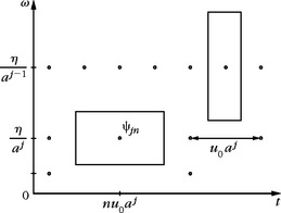
FIGURE 5.5 The Heisenberg box of a wavelet ψj,n scaled by s = aj has a time and frequency width proportional to aj and a−j, respectively. The time-frequency plane is covered by these boxes if u0 and a are sufficiently small.
In the following, we give without proof, some necessary conditions and sufficient conditions on ψ, a and u0 so that {ψj,n}(j,n)∈![]() 2 is a frame of L2(
2 is a frame of L2(![]() ).
).
Necessary Conditions
We suppose that ψ is real, normalized, and satisfies the admissibility condition of Theorem 4.4:
Theorem 5.15:
Daubechies. If {ψj,n}(j,n)∈![]() 2 is a frame of L2(
2 is a frame of L2(![]() ), then the frame bounds satisfy
), then the frame bounds satisfy
This theorem is proved in [19, 163]. Condition (5.77) is equivalent to the frame condition (5.55) for a translation-invariant dyadic wavelet transform, for which the parameter u is not sampled. It requires that the Fourier axis is covered by wavelets dilated by {aj}j∈![]() . The inequality (5.76), which relates the sampling density u0 loge a to the frame bounds, is proved in [19]. It shows that the frame is an orthonormal basis if and only if
. The inequality (5.76), which relates the sampling density u0 loge a to the frame bounds, is proved in [19]. It shows that the frame is an orthonormal basis if and only if
Chapter 7 constructs wavelet orthonormal bases of L2(![]() ) with regular wavelets of compact support.
) with regular wavelets of compact support.
Sufficient Conditions
Theorem 5.16 proved by Daubechies [19] provides a lower and upper bound for the frame bounds A and B, depending on ψ, u0, and a.
Theorem 5.16.
 (5.79)
 (5.80)
then {ψj,n}(j,n)∈![]() 2 is a frame of L2(
2 is a frame of L2(![]() ). The constants A0 and B0 are respectively lower and upper bounds of the frame bounds A and B.
). The constants A0 and B0 are respectively lower and upper bounds of the frame bounds A and B.
The sufficient conditions (5.79) and (5.80) are similar to the necessary condition (5.77). If Δ is small relative to inf![]() , then A0 and B0 are close to the optimal frame bounds A and B. For a fixed dilation step a, the value of Δ decreases when the time-sampling interval u0 decreases.
, then A0 and B0 are close to the optimal frame bounds A and B. For a fixed dilation step a, the value of Δ decreases when the time-sampling interval u0 decreases.
Dual Frame
Theorem 5.5 gives a general formula for computing the dual-wavelet frame vectors
One could reasonably hope that the dual functions ![]() would be obtained by scaling and translating a dual wavelet
would be obtained by scaling and translating a dual wavelet ![]() . The unfortunate reality is that this is generally not true. In general, the operator Φ*Φ does not commute with dilations by aj, so (Φ*Φ)−1 does not commute with these dilations either. On the other hand, one can prove that (Φ*Φ)−1 commutes with translations by naju0, which means that
. The unfortunate reality is that this is generally not true. In general, the operator Φ*Φ does not commute with dilations by aj, so (Φ*Φ)−1 does not commute with these dilations either. On the other hand, one can prove that (Φ*Φ)−1 commutes with translations by naju0, which means that
Thus, the dual frame ![]() is obtained by calculating each elementary function
is obtained by calculating each elementary function ![]() with (5.81), and translating them with (5.82). The situation is much simpler for tight frames, where the dual frame is equal to the original wavelet frame.
with (5.81), and translating them with (5.82). The situation is much simpler for tight frames, where the dual frame is equal to the original wavelet frame.
Mexican Hat Wavelet
The normalized second derivative of a Gaussian is
The graph of these functions is shown in Figure 4.6.
The dilation step a is generally set to be a = 21/v where v is the number of intermediate scales (voices) for each octave. Table 5.2 gives the estimated frame bounds A0 and B0 computed by Daubechies [19] with the formula of Theorem 5.16. For v ≥ 2 voices per octave, the frame is nearly tight when u0 ≤ 0.5, in which case the dual frame can be approximated by the original wavelet frame. As expected from (5.76), when A ≈ B,

The frame bounds increase proportionally to v/u0. For a = 2, we see that A0 decreases brutally from u0 = 1 to u0 = 1.5. For u0 = 1.75, the wavelet family is not a frame anymore. For a = 21/2, the same transition appears for a larger u0.
5.4 WINDOWED FOURIER FRAMES
Frame theory gives conditions for discretizing the windowed Fourier transform while retaining a complete and stable representation. The windowed Fourier transform of f ∈ L2(![]() ) is defined in Section 4.2 by
) is defined in Section 4.2 by
Setting ‖g‖ = 1 implies that ‖gu,ξ‖ = 1. A discrete windowed Fourier transform representation
is complete and stable if {gu, n, ξk}(n,k)∈![]() 2 is a frame of L2(
2 is a frame of L2(![]() ).
).
Intuitively, one can expect that the discrete windowed Fourier transform is complete if the Heisenberg boxes of all atoms {gu, n, ξk}(n,k)∈![]() 2 fully cover the time-frequency plane. Section 4.2 shows that the Heisenberg box of gun, ξk is centered in the time-frequency plane at (un, ξk). Its size is independent of un and ξk. It depends on the time-frequency spread of the window g. Thus, a complete cover of the plane is obtained by translating these boxes over a uniform rectangular grid, as illustrated in Figure 5.6. The time and frequency parameters (u, ξ) are discretized over a rectangular grid with time and frequency intervals of size u0 and ξ0. Let us denote
2 fully cover the time-frequency plane. Section 4.2 shows that the Heisenberg box of gun, ξk is centered in the time-frequency plane at (un, ξk). Its size is independent of un and ξk. It depends on the time-frequency spread of the window g. Thus, a complete cover of the plane is obtained by translating these boxes over a uniform rectangular grid, as illustrated in Figure 5.6. The time and frequency parameters (u, ξ) are discretized over a rectangular grid with time and frequency intervals of size u0 and ξ0. Let us denote

FIGURE 5.6 A windowed Fourier frame is obtained by covering the time-frequency plane with a regular grid of windowed Fourier atoms, translated by un = n u0 in time and by ξk = k ξ0 in frequency.
The sampling intervals (u0, ξ0) must be adjusted to the time-frequency spread of g.
Window Scaling
Suppose that {gn,k}(n,k)∈![]() 2 is a frame of L2(
2 is a frame of L2(![]() ) with frame bounds A and B. Let us dilate the window gs(t) = s−1/2g(t/s). It increases by s the time width of the Heisenberg box of g and reduces by s its frequency width. Thus, we obtain the same cover of the time-frequency plane by increasing u0 by s and reducing ξ0 by s. Let
) with frame bounds A and B. Let us dilate the window gs(t) = s−1/2g(t/s). It increases by s the time width of the Heisenberg box of g and reduces by s its frequency width. Thus, we obtain the same cover of the time-frequency plane by increasing u0 by s and reducing ξ0 by s. Let
We prove that {gs,n,k}(n,k)∈![]() 2 satisfies the same frame inequalities as {gn,k}(n,k)∈
2 satisfies the same frame inequalities as {gn,k}(n,k)∈![]() 2, with the same frame bounds A and B, by a change of variable t′ = ts in the inner product integrals.
2, with the same frame bounds A and B, by a change of variable t′ = ts in the inner product integrals.
5.4.1 Tight Frames
Tight frames are easier to manipulate numerically since the dual frame is equal to the original frame. Daubechies, Grossmann, and Meyer [197] give sufficient conditions for building a window of compact support that generates a tight frame.
Theorem 5.17:
Daubechies, Grossmann, Meyer. Let g be a window that has a support included in [−π/ξ0, π/ξ0]. If
then {gn,k(t) = g(t − nu0) eikξ0t}(n,k)∈![]() 2 is a tight frame L2(
2 is a tight frame L2(![]() ) with a frame bound equal to A.
) with a frame bound equal to A.
Proof.
The function g(t − nu0)f(t) has a support in [nu0 − π/ξ0, nu0 + π/ξ0]. Since {eikξ0t}k∈![]() is an orthogonal basis of this space, we have
is an orthogonal basis of this space, we have

Since gn,k(t) = g(t − nu0)eikξ0t, we get
Summing over n and inserting (5.85) proves that A ‖f‖2 = Σ+∞k,n = −∞ |〈f, gn, k〉|2, and therefore, that {gn,k}(n,k)∈![]() 2 is a tight frame of L2(
2 is a tight frame of L2(![]() ).
).
Since g has a support in [−π/ξ0, π/ξ0] the condition (5.85) implies that
so that there is no whole between consecutive windows g(t − nu0) and g(t − (n + 1)u0). If we impose that 1 ≤ 2π/(u0ξ0) ≤ 2, then only consecutive windows have supports that overlap. The square root of a Hanning window
is a positive normalized window that satisfies (5.85) with u0 = π/ξ0 and a redundancy factor of A = 2. The design of other windows is studied in Section 8.4.2 for local cosine bases.
Discrete Window Fourier Tight Frames
To construct a windowed Fourier tight frame of ![]() N, the Fourier basis {eikξ0t}k∈
N, the Fourier basis {eikξ0t}k∈![]() of L2[−π/ξ0, π/ξ0] is replaced by the discrete Fourier basis {ei2πkn/K}0≤k<K of
of L2[−π/ξ0, π/ξ0] is replaced by the discrete Fourier basis {ei2πkn/K}0≤k<K of ![]() K. Theorem 5.18 is a discrete equivalent of Theorem 5.17.
K. Theorem 5.18 is a discrete equivalent of Theorem 5.17.
Theorem 5.18.
Let g[n] be an N periodic discrete window with a support and restricted to [−N/2, N/2] that is included in [−K/2, K/2 − 1]. If M divides N and
then {gm,k[n] = g[n − mM]ei2πkn/K}0≤k<K, 0≥m<N/M is a tight frame ![]() N with a frame bound equal to A.
N with a frame bound equal to A.
The proof of this theorem follows the same steps as the proof of Theorem 5.17. It is left in Exercise 5.10. There are N/M translated windows and thus NK/M windowed Fourier coefficients. For a fixed window position indexed by m, the discrete windowed Fourier coefficients are the discrete Fourier coefficients of the windowed signal
They are computed with O(K log2 K) operations with an FFT Overall windows, this requires a total of O(NK/M log2 K) operations. We generally choose 1 < K/M ≤ 2 so that only consecutive windows overlap. The square root of a Hanning window g[n] = √2/K cos(πn/K) satisfies (5.86) for M = K/2 and a redundancy factor A = 2. Figure 5.7 shows the log spectrogram log |Sf[m, k]|2 of the windowed Fourier frame coefficients computed with a square root Hanning window for a musical recording.

5.4.2 General Frames
For general windowed Fourier frames of L2(![]() 2), Daubechies [19] proved several necessary conditions on g, u0 and ξ0 to guarantee that {gn,k}(n,k)∈
2), Daubechies [19] proved several necessary conditions on g, u0 and ξ0 to guarantee that {gn,k}(n,k)∈![]() 2 is a frame of L2(
2 is a frame of L2(![]() ). We do not reproduce the proofs, but summarize the main results.
). We do not reproduce the proofs, but summarize the main results.
Theorem 5.19:
Daubechies. The windowed Fourier family {gn,k}(n,k)∈![]() 2 is a frame only if
2 is a frame only if
The frame bounds A and B necessarily satisfy
The ratio 2π/(u0ξ0) measures the density of windowed Fourier atoms in the time-frequency plane. The first condition (5.87) ensures that this density is greater than 1 because the covering ability of each atom is limited. Inequalities (5.89) and (5.90) are proved in full generality by Chui and Shi [163]. They show that the uniform time translations of g must completely cover the time axis, and the frequency translations of its Fourier transform ĝ must similarly cover the frequency axis.
Since all windowed Fourier vectors are normalized, the frame is an orthogonal basis only if A = B = 1. The frame bound condition (5.88) shows that this is possible only at the critical sampling density u0ξ0 = 2π. The Balian-Low Theorem 5.20 [93] proves that g is then either nonsmooth or has a slow time decay.
Theorem 5.20.
Balian-Low. If {gn,k}(n,k)∈![]() 2 is a windowed Fourier frame with u0ξ0 = 2π, then
2 is a windowed Fourier frame with u0ξ0 = 2π, then
This theorem proves that we cannot construct an orthogonal windowed Fourier basis with a differentiable window g of compact support. On the other hand, one can verify that the discontinuous rectangular window
yields an orthogonal windowed Fourier basis for u0ξ0 = 2π. This basis is rarely used because of the bad frequency localization of g.
Sufficient Conditions
Theorem 5.21 proved by Daubechies [195] gives sufficient conditions on u0ξ0, and g for constructing a windowed Fourier frame.
Theorem 5.21:
 (5.93)
then {gn,k}(n,k)∈![]() 2 is a frame. The constants A0 and B0 are, respectively, lower bounds and upper bounds of the frame bounds A and B.
2 is a frame. The constants A0 and B0 are, respectively, lower bounds and upper bounds of the frame bounds A and B.
Observe that the only difference between the sufficient conditions (5.94, 5.95) and the necessary condition (5.89) is the addition and subtraction of Δ. If Δ is small compared to inf0≤t≤u0 Σ+∞n=−∞ |g(t − nu0)|2, then A0 and B0 are close to the optimal frame bounds A and B.
Dual Frame
Theorem 5.5 proves that the dual-windowed frame vectors are
Theorem 5.22 shows that this dual frame is also a windowed Fourier frame, which means that its vectors are time and frequency translations of a new window ĝ.
Theorem 5.22.
Dual-windowed Fourier vectors can be rewritten as
Proof.
This result is proved by showing first that Φ*Φ commutes with time and frequency translations proportional to u0 and ξ0. If φ ∈ L2(![]() ) and φm,l(t) = φ(t − mu0) exp(ilξ0t), we verify that
) and φm,l(t) = φ(t − mu0) exp(ilξ0t), we verify that
and a change of variable yields
Since Φ*Φ commutes with these translations and frequency modulations, we verify that (Φ*Φ)−1 necessarily commutes with the same group operations. Thus,
Gaussian Window
has a Fourier transform ĝ that is a Gaussian with the same variance. The time and frequency spreads of this window are identical. Therefore, let us choose equal sampling intervals in time and frequency: u0 = ξ0. For the same product u0ξ0 other choices would degrade the frame bounds. If g is dilated by s then the time and frequency sampling intervals must become su0 and ξ0/s.
If the time-frequency sampling density is above the critical value of 2π/(u0ξ0) > 1, then Daubechies [195] proves that {gn,k}(n,k)∈![]() 2 is a frame. When u0ξ0 tends to 2π, the frame bound A tends to 0. For u0ξ0 = 2π, the family {gn,k}(n,k)∈
2 is a frame. When u0ξ0 tends to 2π, the frame bound A tends to 0. For u0ξ0 = 2π, the family {gn,k}(n,k)∈![]() 2 is complete in L2(
2 is complete in L2(![]() ), which means that any f ∈ L2(
), which means that any f ∈ L2(![]() ) is entirely characterized by the inner products {〈f, gn,k〉}(n,k)∈
) is entirely characterized by the inner products {〈f, gn,k〉}(n,k)∈![]() 2. However, the Balian-Low theorem (5.20) proves that it cannot be a frame and one can indeed verify that A = 0 [195]. This means that the reconstruction of f from these inner products is unstable.
2. However, the Balian-Low theorem (5.20) proves that it cannot be a frame and one can indeed verify that A = 0 [195]. This means that the reconstruction of f from these inner products is unstable.
Table 5.3 gives the estimated frame bounds A0 and B0 calculated with Theorem 5.21, for different values of u0 = ξ0. For u0ξ0 = π/2, which corresponds to time and frequency sampling intervals that are half the critical sampling rate, the frame is nearly tight. As expected, A ≈ B ≈ 4, which verifies that the redundancy factor is 4 (2 in time and 2 in frequency). Since the frame is almost tight, the dual frame is approximately equal to the original frame, which means that ![]() When u0ξ0 increases we see that A decreases to zero and
When u0ξ0 increases we see that A decreases to zero and ![]() deviates more and more from a Gaussian. In the limit u0ξ0 = 2π, the dual window
deviates more and more from a Gaussian. In the limit u0ξ0 = 2π, the dual window ![]() is a discontinuous function that does not belong to L2(
is a discontinuous function that does not belong to L2(![]() ). These results can be extended to discrete windowed Fourier transforms computed with a discretized Gaussian window [501].
). These results can be extended to discrete windowed Fourier transforms computed with a discretized Gaussian window [501].
Table 5.3 Frame Bounds for the Gaussian Window (5.98) and u0 = ξ0

5.5 MULTISCALE DIRECTIONAL FRAMES FOR IMAGES
To reveal geometric image properties, wavelet frames are constructed with mother wavelets having a direction selectivity, providing information on the direction of sharp transitions such as edges and textures. Directional wavelet frames are described in Section 5.5.1.
Wavelet frames yield high-amplitude coefficients in the neighborhood of edges, and cannot take advantage of their geometric regularity to improve the sparsity of the representation. Curvelet frames, described in Section 5.5.2, are constructed with elongated waveforms that follow directional image structures and improve the representation sparsity.
5.5.1 Directional Wavelet Frames
A directional wavelet transform decomposes images over directional wavelets that are translated, rotated, and dilated at dyadic scales. Such transforms appear in many image-processing applications and physiological models. Applications to texture discrimination are also discussed.
A directional wavelet ψα(x) with x = (x1, x2) ∈ ![]() 2 of angle α is a wavelet having p directional vanishing moments along any one-dimensional line of direction α + π/2 in the plane
2 of angle α is a wavelet having p directional vanishing moments along any one-dimensional line of direction α + π/2 in the plane
but does not have directional vanishing moments along the direction α. Such a wavelet oscillates in the direction of α + π/2 but not in the direction α. It is orthogonal to any two-dimensional polynomial of degree strictly smaller than p (Exercise 5.21).
The set Θ of chosen directions are typically uniform in [0, π]: Θ = {α = kπ/K for 0 ≤ k < K}. Dilating these directional wavelets by factors 2j and translating them by any u ∈ ![]() yields a translation-invariant directional wavelet family:
yields a translation-invariant directional wavelet family:
Directional wavelets may be derived by rotating a single mother wavelet ψ(x1, x2) having vanishing moments in the horizontal direction, with a rotation operator Rα of angle α in ![]() 2.
2.
A dyadic directional wavelet transform of f computes the inner product with each wavelet:
This dyadic wavelet transform can also be written as convolutions with directional wavelets:
A wavelet ψα2j (x − u) has a support dilated by 2j, located in the neighborhood of u and oscillates in the direction of α + π/2. If f(x) is constant over the support of ψα2j, u along lines of direction α + π/2, then 〈f, ψα2j, u〉 = 0 because of its directional vanishing moments. In particular, this coefficient vanishes in the neighborhood of an edge having a tangent in the direction α + π/2. If the edge angle deviates from α + π/2, then it produces large amplitude coefficients, with a maximum typically when the edge has a direction α. Thus, the amplitude of wavelet coefficients depends on the local orientation of the image structures.
Theorem 5.11 proves that the translation-invariant wavelet family is a frame if there exists B ≥ A > 0 such that the generators φn(x) = 2−jψα2j (x) have Fourier transforms ![]() , which satisfy
, which satisfy
It results from Theorem 5.11 that there exists a dual family of reconstructing wavelets ![]() that have Fourier transforms that satisfy
that have Fourier transforms that satisfy
Examples of directional wavelets obtained by rotating a single mother wavelet are constructed with Gabor functions and steerable derivatives.
Gabor Wavelets
In the cat’s visual cortex, Hubel and Wiesel [306] discovered a class of cells, called simple cells, having a response that depends on the frequency and direction of the visual stimuli. Numerous physiological experiments [401] have shown that these cells can be modeled as linear filters with impulse responses that have been measured at different locations of the visual cortex. Daugmann [200] showed that these impulse responses can be approximated by Gabor wavelets, obtained with a Gaussian window ![]() multiplied by a sinusoidal wave:
multiplied by a sinusoidal wave:
These findings suggest the existence of some sort of wavelet transform in the visual cortex, combined with subsequent nonlinearities [403]. The “physiological” wavelets have a frequency resolution on the order of 1 to 1.5 octaves, and are thus similar to dyadic wavelets.
The Fourier transform of g(x1, x2) is ![]() . It results from (5.104) that
. It results from (5.104) that
In the Fourier plane, the energy of this Gabor wavelet is mostly concentrated around (−2−j η sin α, 2−j η cos α), in a neighborhood proportional to 2−j.
The direction is chosen to be uniform a = lπ/K for −K < l ≤ K. Figure 5.8 shows a cover of the frequency plane by dyadic Gabor wavelets 5.105 with K = 6. If K ≥ 4 and η is of the order of 1 then 5.101 is satisfied with stable bounds. Since images f(x) are real, ![]() and f can be reconstructed by covering only half of the frequency plane, with −K < l ≤ 0. This is a two-dimensional equivalent of the one-dimensional analytic wavelet transform, studied in Section 4.3.2, with wavelets having a Fourier transform support restricted to positive frequencies. For texture analysis, Gabor wavelets provide information on the local image frequencies.
and f can be reconstructed by covering only half of the frequency plane, with −K < l ≤ 0. This is a two-dimensional equivalent of the one-dimensional analytic wavelet transform, studied in Section 4.3.2, with wavelets having a Fourier transform support restricted to positive frequencies. For texture analysis, Gabor wavelets provide information on the local image frequencies.

Texture Discrimination
Despite many attempts, there are no appropriate mathematical models for “homogeneous image textures.” The notion of texture homogeneity is still defined with respect to our visual perception. A texture is said to be homogeneous if it is preattentively perceived as being homogeneous by a human observer.
The texton theory of Julesz [322] was a first important step in understanding the different parameters that influence the perception of textures. The direction of texture elements and their frequency content seem to be important clues for discrimination. This motivated early researchers to study the repartition of texture energy in the Fourier domain [92]. For segmentation purposes it is necessary to localize texture measurements over neighborhoods of varying sizes. Thus, the Fourier transform was replaced by localized energy measurements at the output of filter banks that compute a wavelet transform [315, 338, 402, 467]. Besides the algorithmic efficiency of this approach, this model is partly supported by physiological studies of the visual cortex.
Since ![]() , Gabor wavelet coefficients measure the energy of f in a spatial neighborhood of u of size 2j, and in a frequency neighborhood of (−2−j η sin α, 2−j η cos α) of size 2−j, where the support of
, Gabor wavelet coefficients measure the energy of f in a spatial neighborhood of u of size 2j, and in a frequency neighborhood of (−2−j η sin α, 2−j η cos α) of size 2−j, where the support of ![]() is located, illustrated in Figure 5.8. Varying the scale 2j and the angle α modifies the frequency channel [119]. The wavelet transform energy |W f(u, 2j, α)|2 is large when the angle α and scale 2j match the direction and scale of high-energy texture components in the neighborhood of u. Thus, the amplitude of |W f(u, 2j, α)|2 can be used to discriminate textures. Figure 5.9 shows the dyadic wavelet transform of two textures, computed along horizontal and vertical directions, at the scales 2−4 and 2−5 (the image support is normalized to [0, 1]2). The central texture is regular vertically and has more energy along horizontal high frequencies than the peripheric texture. These two textures are therefore discriminated by the wavelet of angle α = π/2, whereas the other wavelet with α = 0 produces similar responses for both textures.
is located, illustrated in Figure 5.8. Varying the scale 2j and the angle α modifies the frequency channel [119]. The wavelet transform energy |W f(u, 2j, α)|2 is large when the angle α and scale 2j match the direction and scale of high-energy texture components in the neighborhood of u. Thus, the amplitude of |W f(u, 2j, α)|2 can be used to discriminate textures. Figure 5.9 shows the dyadic wavelet transform of two textures, computed along horizontal and vertical directions, at the scales 2−4 and 2−5 (the image support is normalized to [0, 1]2). The central texture is regular vertically and has more energy along horizontal high frequencies than the peripheric texture. These two textures are therefore discriminated by the wavelet of angle α = π/2, whereas the other wavelet with α = 0 produces similar responses for both textures.
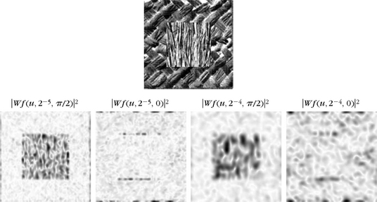
FIGURE 5.9 Directional Gabor wavelet transform |W f(u, 2j, α)|2 of a texture patch, at the scales 2j = 2−4, 2−5, along two directions α = 0, π/2. The darker the pixel, the larger the wavelet coefficient amplitude.
For segmentation, one must design an algorithm that aggregates the wavelet responses at all scales and directions in order to find the boundaries of homogeneous textured regions. Both clustering procedures and detection of sharp transitions over wavelet energy measurements have been used to segment the image [315, 402, 467]. These algorithms work well experimentally but rely on ad hoc parameter settings.
Steerable Wavelets
Steerable directional wavelets along any angle α can be written as a linear expansion of few mother wavelets [441]. For example, a steerable wavelet in the direction α can be defined as the partial derivative of order p of a window p(x) in the direction of the vector ![]() = (− sin α, cos α):
= (− sin α, cos α):
Let Rα be the planar rotation by an angle α. If the window is invariant under rotations θ(x) = θ(Rαx), then these wavelets are generated by the rotation of a single mother wavelet: ψα(x) = ψ(Rαx) with ψ = ∂pθ/∂xp2.
Furthermore, the expansion of the derivatives in (5.105) proves that each ψα can be expressed as a linear combination of p + 1 partial derivatives
The waveforms ρi (x) can also be considered as wavelets functions with vanishing moments. It results from 5.106 that the directional wavelet transform at any angle α can be calculated from p + 1 convolutions of f with the ρi dilated:
Exercise 5.22 gives conditions on θ so that for a set θ of p + 1 angles α = kπ/(p + 1) with 0 ≤ k < p the resulting oriented wavelets ψα define a family of dyadic wavelets that satisfy 5.101. Section 6.3 uses such directional wavelets, with p = 1, to detect multiscale edges in images.
Discretization of the Translation
A translation-invariant wavelet transforms W f(u, 2j, α) for all scales 2j, and angle α requires a large amount of memory. To reduce computation and memory storage, the translation parameter is discretized. In the one-dimensional case a frame is obtained by uniformly sampling the translation parameter u with intervals u02j n with n = (n1, n2) ∈ ![]() 2, proportional to the scale 2j. The discretized wavelet derived from the translation-invariant wavelet family (5.100) is
2, proportional to the scale 2j. The discretized wavelet derived from the translation-invariant wavelet family (5.100) is
Necessary and sufficient conditions similar to Theorems 5.15 and 5.16 can be established to guarantee that such a wavelet family defines a frame of L2(![]() 2).
2).
To decompose images in such wavelet frames with a fast filter filter bank, directional wavelets can be synthesized as a product of discrete filters. The steerable pyramid of Simoncelli et al. [441] decomposes images in such a directional wavelet frame, with a cascade of convolutions with low-pass filters and directional band-pass filters. The filter coefficients are optimized to yield wavelets that satisfy approximately the steerability condition 5.106 and produce a tight frame. The sampling interval is u0 = 1/2.
Figure 5.10 shows an example of decomposition on such a steerable pyramid with K = 4 directions. For discrete images of N pixels, the finest scale is 2j = 2N−1. Since u0 = 1/2, wavelet coefficients at the finest scale define an image of N pixels for each direction. The wavelet image size then decreases as the scale 2j increases. The total number of wavelet coefficients is 4KN/3 and the tight frame factor is 4K/3 [441]. Steerable wavelet frames are used to remove noise with wavelet thresholding estimators [404] and for texture analysis and synthesis [438].

FIGURE 5.10 Decomposition of an image in a frame of steerable directional wavelets [441] along four directions: α = 0, π/4, π/2, 3π/4, at two consecutive scales, 2j and 2j + 1. Black, gray, and white pixels correspond respectively to wavelet coefficients of negative, zero, and positive values.
Chapter 9 explains that sparse image representation can be obtained by keeping large-amplitude coefficients above a threshold. Large-amplitude wavelet coefficients appear where the image has a sharp transition, when the wavelet oscillates in a direction approximately perpendicular to the direction of the edge. However, even when directions are not perfectly aligned, wavelet coefficients remain nonnegligible in the neighborhood of edges. Thus, the number of large-amplitude wavelet coefficients is typically proportional to the length of edges in images. Reducing the number of large coefficients requires using waveforms that are more sensitive to direction properties, as shown in the next section.
5.5.2 Curvelet Frames
Curvelet frames were introduced by Candès and Donoho [134] to construct sparse representation for images including edges that are geometrically regular. Similar to directional wavelets, curvelet frames are obtained by rotating, dilating, and translating elementary waveforms. However, curvelets have a highly elongated support obtained with a parabolic scaling using different scaling factors along the curvelet width and length. These anisotropic waveforms have a much better direction sensitivity than directional wavelets. Section 9.3.2 studies applications to sparse approximations of geometrically regular images.
Dyadic Curvelet Transform
A curvelet is function c(x) having vanishing moments along the horizontal direction like a wavelet. However, as opposed to wavelets, dilated curvelets are obtained with a parabolic scaling law that produces highly elongated waveforms at fine scales:
They have a width proportional to their length2. Dilated curvelets are then rotated cα2j = c2j (Rαx), where Rα is the planar rotation of angle α, and translated like wavelets: cα2j, u = cα2j (x − u). The resulting translation-invariant dyadic curvelet transform of f ∈ L2(![]() 2) is defined by
2) is defined by
To obtain a tight frame, the Fourier transform of a curvelet at a scale 2j is defined by
where ![]() is the Fourier transform of a one-dimensional wavelet and
is the Fourier transform of a one-dimensional wavelet and ![]() is a one-dimensional angular window that localizes the frequency support of ĉ2j in a polar parabolic wedge, illustrated in Figure 5.11. The wavelet
is a one-dimensional angular window that localizes the frequency support of ĉ2j in a polar parabolic wedge, illustrated in Figure 5.11. The wavelet ![]() is chosen to have a compact support in [1/2, 2] and satisfies the dyadic frequency covering:
is chosen to have a compact support in [1/2, 2] and satisfies the dyadic frequency covering:
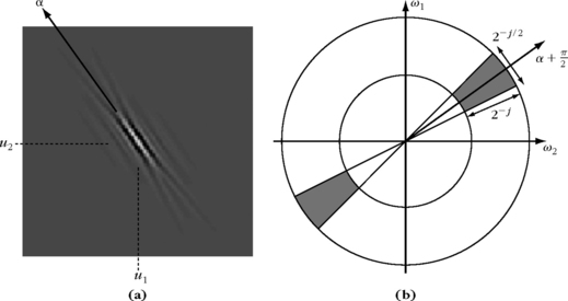
FIGURE 5.11 (a) Example of curvelet cα2j, u (x). (b) The frequency support of ĉα2j, u (ω) is a wedge obtained as a product of a radial window with an angular window.
One may, for example, choose a Meyer wavelet as defined in (7.82). The angular window ![]() is chosen to be supported in [−1, 1] and satisfies
is chosen to be supported in [−1, 1] and satisfies
As a result of these two properties, one can verify that for uniformly distributed angles,
curvelets cover the frequency plane
Real valued curvelets are obtained with a symmetric version of 5.109: ĉ2j (ω) + ĉ2j (−ω). Applying Theorem 5.11 proves that a translation-invariant dyadic curvelet dictionary {cα2j, u}α∈θj, j∈![]() , u∈
, u∈![]() 2 is a dyadic translation-invariant tight frame that defines a complete and stable signal representation [142].
2 is a dyadic translation-invariant tight frame that defines a complete and stable signal representation [142].
Curvelet Properties
Since ĉ2j(ω) is a smooth function with a support included in a rectangle of size proportional to 2−j/2 × 2−j, the spatial curvelet c2j (x) is a regular function with a fast decay outside a rectangle of size 2−j/2 × 2j. The rotated and translated curvelet cα2j, u is supported around the point u in an elongated rectangle along the direction α; its shape has a parabolic ratio width = length2, as shown in Figure 5.11.
Since the Fourier transform ĉ2j (Ω1, Ω2) is zero in the neighborhood of the vertical axis Ω1 = 0, c2j(x1, x2) has an infinite number of vanishing moments in the horizontal direction
A rotated curvelet cα2j, u has vanishing moments in the direction α + π/2, and therefore oscillates in the direction α + π/2, whereas its support is elongated in the direction α.
Discretization of Translation
Curvelet tight frames are constructed by sampling the translation parameter u [134]. These tight frames provide sparse representations of signals including regular geometric structures.
The curvelet sampling grid depends on the scale 2j and on the angle α. Sampling intervals are proportional to the curvelet width 2j in the direction α + π/2 and to its length 2j/2 in the direction α:
Figure 5.12 illustrates this sampling grid. The resulting dictionary of translated curvelets is
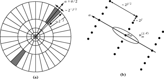
FIGURE 5.12 (a) Curvelet polar tiling of the frequency plane with parabolic wedges. (b) Curvelet spatial sampling grid u(j,α)m at a scale 2j and direction α.
Theorem 5.24 proves that this curvelet family is a tight frame of L2(![]() 2). The proof is not given here, but can be found in [142].
2). The proof is not given here, but can be found in [142].
Wavelet versus Curvelet Coefficients
In the neighborhood of an edge having a tangent in a direction θ, large-amplitude coefficients are created by curvelets and wavelets of direction α = θ, which have their vanishing moment in the direction θ + π/2. These curvelets have a support elongated in the edge direction θ, as illustrated in Figure 5.13. In this direction, the sampling grid of a curvelet frame has an interval 2j/2, which is much larger than the sampling interval 2j of a wavelet frame. Thus, an edge is covered by fewer curvelets than wavelets having a direction equal to the edge direction. If the angle α of the curvelet deviates from 0, then curvelet coefficients decay quickly because of the narrow frequency localizaton of curvelets. This gives a high-directional selectivity to curvelets.

FIGURE 5.13 (a) Directional wavelets: a regular edge creates more large-amplitude wavelet coefficients than curvelet coefficients. (b) Curvelet coefficients have a large amplitude when their support is aligned with the edge direction, but there are few such curvelets.
Even though wavelet coefficients vanish when α = θ + π/2, they have a smaller directional selectivity than curvelets, and wavelet coefficients’ amplitudes decay more slowly as α deviates from θ. Indeed, the frequency support of wavelets is much wider and their spatial support is nearly isotropic. As a consequence, an edge produces large-amplitude wavelet coefficients in several directions. This is illustrated by Figure 5.10, where Lena’s shoulder edge creates large coefficients in three directions, and small coefficients only when the wavelet and the edge directions are aligned.
As a result, edges and image structures with some directional regularity create fewer large-amplitude curvelet coefficients than wavelet coefficients. The theorem derived from Section 933 proves that for images having regular edges, curvelet tight frames are asymptotically more efficient than wavelet bases when building sparse representations.
Fast Curvelet Decomposition Algorithm
To compute the curvelet transform of a discrete image f[n1, n2] uniformly sampled over N pixels, one must take into account the discretization grid, which imposes constraints on curvelet angles. The fast curvelet transform [140] replaces the polar tiling of the Fourier domain by a recto-polar tiling, illustrated in Figure 5.14(b). The directions α are uniformly discretized so that the slopes of the wedges containing the support of the curvelets are uniformly distributed in each of the north, south, west, and east Fourier quadrants. Each wedge is the support of the two-dimensional DFT ĉαj[k1, k2] of a discrete curvelet cαj [n1, n2]. The curvelet translation parameters are not chosen according to 5.113, but remain on a subgrid of the original image sampling grid. At a scale 2j, there is one sampling grid (2⌋j/2⌊m1, 2j m2) for curvelets in the east and west quadrants. In these directions, curvelet coefficients are
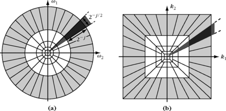
FIGURE 5.14 (a) Curvelet frequency plane tiling. The dark gray area is a wedge obtained as the product of a radial window and an angular window. (b) Discrete curvelet frequency tiling. The radial and angular windows define trapezoidal wedges as shown in dark gray.
with ![]() . For curvelets in the north and south quadrants the translation grid is (2j m1, 2⌋j/2⌊ m2), which corresponds to curvelet coefficients
. For curvelets in the north and south quadrants the translation grid is (2j m1, 2⌋j/2⌊ m2), which corresponds to curvelet coefficients
The discrete curvelet transform computes the curvelet filtering and sampling with a two-dimensional FFT. The two-dimensional discrete Fourier transforms of f[n] and ![]() are
are ![]() and
and ![]() [k]. The algorithm proceeds as:
[k]. The algorithm proceeds as:
• Computation of the two-dimensional DFT ![]() [k] of f[n].
[k] of f[n].
• For each j and the corresponding 2−⌋j/2⌊ + 2 angles α, calculation of ![]() .
.
• Computation of the inverse Fourier transform of ![]() on the smallest possible warped frequency rectangle including the wedge support of
on the smallest possible warped frequency rectangle including the wedge support of ![]() .
.
The critical step is the last inverse Fourier transform. A computationally more expensive one would compute ![]() for all n = (n1, n2) and then subsample this convolution along the grids (5.115) and (5.116).
for all n = (n1, n2) and then subsample this convolution along the grids (5.115) and (5.116).
Instead, the subsampled curvelet coefficients are calculated directly by restricting the FFT to a bounding box that contains the support of ĉαj [−k]. A horizontal or vertical warping maps this bounding box to an elongated rectangular frequency box on which the inverse FFT is calculated. One can verify that the resulting coefficients correspond to the subsampled curvelet coefficients. The overall complexity of the algorithm is then O(N log2 (N)), as detailed in [140]. The tight frame redundancy bound obtained with this discrete algorithm is A ≈ 5.
An orthogonal curvelet type transform has been developed by Do and Vetterli [212]. The resulting contourlets are not redundant but do not have the appropriate time and frequency localization needed to obtain asymptotic approximation results similar to curvelets.
5.6 EXERCISES
5.1. 1 Prove that if K ∈ ![]() − {0}, then {φp[n] = exp (i2πpn/(KN))}0≤p<KN is a tight frame of
− {0}, then {φp[n] = exp (i2πpn/(KN))}0≤p<KN is a tight frame of ![]() N. Compute the frame bound.
N. Compute the frame bound.
5.2. 1 Prove that if K ∈ ![]() − {0}, then {φp(t) = exp (i2πpnt/K)}p∈
− {0}, then {φp(t) = exp (i2πpnt/K)}p∈![]() is a tight frame of L2[0, 1]. Compute the frame bound.
is a tight frame of L2[0, 1]. Compute the frame bound.
5.3. 2 Prove that a finite set of N vectors {φn}1≤n≤N is always a frame of the space V generated by linear combinations of these vectors.
5.4. 1 If U1 and U2 are two operators from ![]() N to
N to ![]() N, prove that the trace (sum of diagonal values) satisfies tr(U1 U2) = tr(U2 U1).
N, prove that the trace (sum of diagonal values) satisfies tr(U1 U2) = tr(U2 U1).
5.5. 2 Prove that the translation-invariant frame
is a translation-invariant frame of the space V = {f ∈ ![]() N : ΣN − 1n = 0 f [n] = 0}. Compute the frame bounds. Is it a numerically stable frame when N is large?
N : ΣN − 1n = 0 f [n] = 0}. Compute the frame bounds. Is it a numerically stable frame when N is large?
5.6. 2 Construct a Riesz basis in ![]() N with a lower frame bound A that tends to zero and an upper frame bound that tends to +∞ as N increases.
N with a lower frame bound A that tends to zero and an upper frame bound that tends to +∞ as N increases.
5.7. 1 If U is an operator from ![]() N to
N to ![]() P, prove that NullU* is the orthogonal complement of ImU in
P, prove that NullU* is the orthogonal complement of ImU in ![]() P.
P.
5.8. 3 Prove Theorem 5.12.
5.9. 1 Let ĝ = 1[−Ω0,Ω0]. Prove that {g(t − p2π/Ω0) exp (ikΩ0t)}(k, p) ∈ ![]() 2 is an orthonormal basis of L2(
2 is an orthonormal basis of L2(![]() ).
).
5.10. 2 Let gm,k[n] = g[n − mM] exp(i2πkn/K), where g[n] is a window with a support included in [−K/2, K/2 − 1].
5.11. 2 Compute the trigonometric polynomials ![]() and
and ![]() of minimum degree that satisfy (5.63) for the spline filters (5.67, 5.68) with m = 2. Compute numerically the graph of
of minimum degree that satisfy (5.63) for the spline filters (5.67, 5.68) with m = 2. Compute numerically the graph of ![]() and
and ![]() . Are they finite-energy functions?
. Are they finite-energy functions?
5.12. 1 Compute a cubic spline dyadic wavelet with two vanishing moments using the filter h defined by (5.67) for m = 3, with a filter g having three nonzero coefficients. Compute in WaveLab the dyadic wavelet transform of the Lady signal with this new wavelet. Calculate ![]() if
if ![]() .
.
5.13. 2 Prove the tight-frame energy conservation (4.29) of a discrete windowed Fourier transform. Derive (4.28) from general tight-frame properties. Compute the resulting discrete windowed Fourier transform reproducing kernel.
5.14. 1 Let {g(t − nβ) exp(ikηt)}(n,k)∈![]() 2 be a windowed Fourier frame defined by g(t) = π−1/4 exp(−t2/2) with β = η and β η < 2π. With the conjugate gradient algorithm of Theorem 5.8, compute numerically the window g(t) that generates the dual frame, for the values of β η in Table 5.3. Compare
2 be a windowed Fourier frame defined by g(t) = π−1/4 exp(−t2/2) with β = η and β η < 2π. With the conjugate gradient algorithm of Theorem 5.8, compute numerically the window g(t) that generates the dual frame, for the values of β η in Table 5.3. Compare ![]() with g and explain why they are progressively more different as β η tends to 2π.
with g and explain why they are progressively more different as β η tends to 2π.
5.15. 2 Sigma-Delta converter. A signal f(t) is sampled and quantized. We suppose that ![]() has a support in [−π/T, π/T].
has a support in [−π/T, π/T].
5.16. 3 Oversampled analog-to-digital conversion. Let φs(t) = s1/2 sin(πt/s)/(πt).
5.17. 1 Let ψ be a dyadic wavelet that satisfies (5.48). Let ![]() 2(L2(
2(L2(![]() )) be the space of sequences {gj(u)}j∈
)) be the space of sequences {gj(u)}j∈![]() such that
such that ![]() .
.
and W−1 be the operator defined by
5.18. 1 Prove that if there exist A > 0 and B ≥ 0 such that
and if φ defined in (5.59) belongs to L2(![]() ), then the wavelet ψ given by (5.60) satisfies the dyadic wavelet condition (5.55).
), then the wavelet ψ given by (5.60) satisfies the dyadic wavelet condition (5.55).
5.19. 3 Zak transform. The Zak transform associates to any f ∈ L2(![]() )
)
by verifying that for g = 1[0, 1], it transforms the orthogonal basis {gn,k(t) = g(t − n) exp(i2πkt)}(n,k)∈![]() 2 of L2(
2 of L2(![]() ) into an orthonormal basis of L2[0, 1]2.
) into an orthonormal basis of L2[0, 1]2.
5.20. 3 Suppose that ![]() has a support in [−π/T, π/T]. Let {f(tn)}n∈
has a support in [−π/T, π/T]. Let {f(tn)}n∈![]() be irregular samples that satisfy (5.8). With the conjugate gradient Theorem 5.8, implement numerically a procedure that computes a uniform sampling {f(nT)}n∈
be irregular samples that satisfy (5.8). With the conjugate gradient Theorem 5.8, implement numerically a procedure that computes a uniform sampling {f(nT)}n∈![]() (from which f can be recovered with the sampling Theorem 3.2). Analyze the convergence rate of the conjugate-gradient algorithm as a function of δ. What happens if the condition (5.8) is not satisfied?
(from which f can be recovered with the sampling Theorem 3.2). Analyze the convergence rate of the conjugate-gradient algorithm as a function of δ. What happens if the condition (5.8) is not satisfied?
5.21. 2 Prove that if ψ(x1, x2) is a directional wavelet having p vanishing moments in a direction α + π/2 as defined in (5.99), then it is orthogonal to any two-dimensional polynomial of degree p − 1.
5.23. 4 Develop a texture classification algorithm with a two-dimensional Gabor wavelet transform using four oriented wavelets. The classification procedure can be based on “feature vectors” that provide local averages of the wavelet transform amplitude at several scales, along these four orientations [315, 338, 402, 467].