
12.5 PURSUIT RECOVERY
Matching pursuits and basis pursuits are nonoptimal sparse approximation algorithms in a redundant dictionary D, but are computationally efficient. However, pursuit approximations can be nearly as precise as optimal M-term approximations, depending on the properties of the approximation supports in D.
Beyond approximation, this section studies the ability of pursuit algorithms to recover a specific set Λ of vectors providing a sparse signal approximation in a redundant dictionary. The stability of this recovery is important for pattern recognition when selected dictionary vectors are used to analyze the signal information. It is also at the core of the sparse super-resolution algorithms introduced in Section 13.3.
The stability of sparse signal approximations in redundant dictionaries is related to the dictionary coherence in Section 12.5.1. The exact recovery of signals with matching pursuits and basis pursuits are studied in Sections 12.5.2 and 12.5.3, together with the precision of M-term approximations.
12.5.1 Stability and Incoherence
Let ![]() be a redundant dictionary of normalized vectors. Given a family of linearly independent approximation vectors
be a redundant dictionary of normalized vectors. Given a family of linearly independent approximation vectors ![]() selected by some algorithm, the best approximation of f is its orthogonal projection fΛ in the space VΛ generated by these vectors
selected by some algorithm, the best approximation of f is its orthogonal projection fΛ in the space VΛ generated by these vectors
The calculation of the coefficients a[p] is stable if ![]() is a Riesz basis of VΛ, with Riesz bounds BΛ ≥ AΛ > 0, which satisfy:
is a Riesz basis of VΛ, with Riesz bounds BΛ ≥ AΛ > 0, which satisfy:
The closer AΛ/BΛ to 1, the more stable the basis. Gradient descent algorithms compute the coefficients a[p] with a convergence rate that also depends on AΛ/BΛ. Theorem 12.10 relates the Riesz bounds to the dictionary mutual coherence, introduced by Donoho and Huo [230],
Theorem 12.10.
Proof.
Theorem 5.1 proves that the constants AΛ and BΛ are lower and upper bounds of the eigenvalues of the Gram matrix ![]() Let v ≠ 0 be an eigenvector satisfying GΛv = λv. Let
Let v ≠ 0 be an eigenvector satisfying GΛv = λv. Let ![]() Since
Since ![]() ,
,

It results that
which proves (12.120).
The Riesz bound ratio AΛ/BΛ is close to 1 if δΛ is small and thus if the vectors in Λ have a small correlation. The upper bound (12.120) proves that sufficiently small sets ![]() are Riesz bases with AΛ > 0. To increase the maximum size of these sets, one should construct dictionaries that are as incoherent as possible. The upper bounds (12.120) are simple but relatively crude, because they only depend on inner products of pairs of vectors, whereas the Riesz stability of
are Riesz bases with AΛ > 0. To increase the maximum size of these sets, one should construct dictionaries that are as incoherent as possible. The upper bounds (12.120) are simple but relatively crude, because they only depend on inner products of pairs of vectors, whereas the Riesz stability of ![]() depends on the distribution of this whole group of vectors on the unit sphere of CN. Section 13.4 proves that much better bounds can be calculated over dictionaries of random vectors.
depends on the distribution of this whole group of vectors on the unit sphere of CN. Section 13.4 proves that much better bounds can be calculated over dictionaries of random vectors.
The mutual coherence of an orthonormal basis D is 0, and one can verify (Exercise 12.5) that if we add a vector g, then ![]() . However, this level of incoherence can be reached with larger dictionaries. Let us consider the dictionary of P = 2N vectors, which is a union of a Dirac basis and a discrete Fourier basis:
. However, this level of incoherence can be reached with larger dictionaries. Let us consider the dictionary of P = 2N vectors, which is a union of a Dirac basis and a discrete Fourier basis:
Its mutual coherence is μ(D) = N−1/2. The right upper bound of (12.120) thus proves that any family of ![]() Dirac and Fourier vectors defines a basis with a Riesz bound ratio AΛ/BΛ ≥ 1/3. One can construct larger frames D of P = N2 vectors, called Grassmannian frames, that have a coherence in
Dirac and Fourier vectors defines a basis with a Riesz bound ratio AΛ/BΛ ≥ 1/3. One can construct larger frames D of P = N2 vectors, called Grassmannian frames, that have a coherence in ![]() [448].
[448].
Dictionaries often do not have a very small coherence, so the inequality ![]() applies to relatively small sets Λ. For example, in the Gabor dictionary Dj,δ defined in (12.77), the mutual coherence μ(D) is maximized by two neighboring Gabor atoms, and the inner product formula (12.81) proves that
applies to relatively small sets Λ. For example, in the Gabor dictionary Dj,δ defined in (12.77), the mutual coherence μ(D) is maximized by two neighboring Gabor atoms, and the inner product formula (12.81) proves that ![]() for δ = 2. The mutual coherence upper bound is therefore useless in this case, but the first upper bound of (12.120) can be used with (12.81) to verify that Gabor atoms that are sufficiently far in time and frequency generate a Riesz basis.
for δ = 2. The mutual coherence upper bound is therefore useless in this case, but the first upper bound of (12.120) can be used with (12.81) to verify that Gabor atoms that are sufficiently far in time and frequency generate a Riesz basis.
12.5.2 Support Recovery with Matching Pursuit
We first study the reconstruction of signals f that have an exact sparse representation in D,
An exact recovery condition on Λ is established to guarantee that a matching pursuit selects only approximation vectors in Λ. The optimality of matching pursuit approximations is then analyzed for more general signals. We suppose that the matching pursuit relaxation factor is α = 1.
An orthogonal matching pursuit, or a matching pursuit with backprojection, computes the orthogonal projection ![]() of f on a family of vectors
of f on a family of vectors ![]() selected one by one. At a step m, a matching pursuit selects an atom in Λ if and only if the correlation of the residual Rmf with vectors in the complement Λc of Λ is smaller than the correlation with vectors in Λ:
selected one by one. At a step m, a matching pursuit selects an atom in Λ if and only if the correlation of the residual Rmf with vectors in the complement Λc of Λ is smaller than the correlation with vectors in Λ:
 (12.122)
The relative correlation of a vector h with vectors in Λc relative to Λ is defined by
Theorem 12.11, proved by Tropp [461], gives a condition that guarantees the recovery of Λ with a matching pursuit.
Theorem 12.11: Tropp. If ![]() is the dual basis of
is the dual basis of ![]() in the space VΛ, then
in the space VΛ, then
If f ∈ VΛ and the following exact recovery condition (ERC) is satisfied,
then a matching pursuit of f selects only vectors in ![]() and an orthogonal matching pursuit recovers f with at most
and an orthogonal matching pursuit recovers f with at most ![]() iterations.
iterations.
Proof.
Let us first prove that suph∈vΛ C(h, Λc) ≤ ERC(Λ). Let ![]() be the pseudo inverse of φΛ with φΛf[p] = f, φp) for p ∈ Λ. Theorem 5.6 proves that
be the pseudo inverse of φΛ with φΛf[p] = f, φp) for p ∈ Λ. Theorem 5.6 proves that ![]() is an orthogonal projector in VΛ, so if h ∈ VΛ and q ∈ Λc,
is an orthogonal projector in VΛ, so if h ∈ VΛ and q ∈ Λc,
 (12.126)
Theorem 5.5 proves that the dual-frame operator satisfies ![]() and thus that
and thus that ![]() for p ∈ Λ. It results that
for p ∈ Λ. It results that
and (12.126) implies that
which proves that ERC(Λ) ≥ suph∈VΛ C(h, Λc).
We now prove the reverse inequality. Let q0 ∈ Λc be the index such that
leads to
Since ![]() , it results that C(h, Λc) ≥ ERC(Λ) and thus suph∈vΛ C(h, Λc) ≥ ERC(Λ), which finishes the proof of (12.124).
, it results that C(h, Λc) ≥ ERC(Λ) and thus suph∈vΛ C(h, Λc) ≥ ERC(Λ), which finishes the proof of (12.124).
Suppose now that f = R0f ∈ VΛ and ERC(Λ) > 1. We prove by induction that a matching pursuit selects only vectors in {φp}p∈Λ. Suppose that the first m < M matching pursuit vectors are in {φp}p∈Λ and thus that Rmf ∈ VΛ. If Rmf ≠ 0, then (12.125) implies that C(Rmf, Λc) < 1 and thus that the next vector is selected in Λ. Since dim (VΛ) ≤ |Λ|, an orthogonal pursuit converges in less than |Λ| iterations.
This theorem proves that if a signal can be exactly decomposed over {φp}p∈Λ, then ERC(Λ) < 1 guarantees that a matching pursuit reconstructs f with vectors in {φp}p∈Λ. A nonorthogonal pursuit may, however, require more than |Λ| iterations to select all vectors in this family.
If ERC(Λ) > 1, then there exists f ∈ VΛ such that C(f, Λc) > 1. As a result, there exists a vector φq with q ∈ Λc, which correlates f better than any other vectors in Λ, and that will be selected by the first iteration of a matching pursuit. This vector may be removed, however, from the approximation support at the end of the decomposition. Indeed, if the remaining iterations select all vectors {φp}p∈Λ, then an orthogonal matching pursuit decomposition or a backprojection will associate a coefficient 0 to φq because f = PVΛf. In particular, we may have ERC(Λ) > 1 but ![]() with
with ![]() , in which case an orthogonal pursuit recovers exactly the support of any f ∈ VΛ with
, in which case an orthogonal pursuit recovers exactly the support of any f ∈ VΛ with ![]() iterations.
iterations.
Theorem 12.12 gives an upper bound proved by Tropp [461], which relates ERC(Λ) to the support size |Λ|. A tighter bound proved by Gribonval and Nielsen [281] and Dossal [231] depends on inner products of dictionary vectors in ã relative to vectors in the complement Λc.
Theorem 12.12: Tropp, Gribonval, Nielsen, Dossal. For any ![]() ,
,
 (12.129)
 Proof.
It is shown in (12.127) that ![]() . We verify that
. We verify that
and thus that we can also write ![]() . Introducing the operator norm associated to the 11 norm
. Introducing the operator norm associated to the 11 norm
for a matrix A = (ai,j)i,j, leads to
The second term is the numerator of (12.129),
The Gram matrix is rewritten as ![]() , and a Neumann expansion of G−1 gives
, and a Neumann expansion of G−1 gives
with
Inserting this result in (12.133) and inserting (12.132) and (12.133) in (12.131) prove the first inequality of (12.129).
The second inequality is derived from the fact that ![]() for any p ≠ q.
for any p ≠ q.
This theorem gives upper bounds of ERC(Λ) that can easily be computed. It proves that ERC(Λ) < 1 if the vectors {φp}p∈Λ are not too correlated between themselves and with the vectors in the complement Λc. In a Gabor dictionary ![]() defined in (12.77), the upper bound (12.129) with the Gabor inner product formula (12.81) proves that ERC(Λ) < 1 for families of sufficiently separated time-frequency Gabor atoms indexed by Λ. Theorem 12.11 proves that any combination of such Gabor atoms is recovered by a matching pursuit. Suppose that the Gabor atoms are defined with a Gaussian window that has a variance in time and frequency that is
defined in (12.77), the upper bound (12.129) with the Gabor inner product formula (12.81) proves that ERC(Λ) < 1 for families of sufficiently separated time-frequency Gabor atoms indexed by Λ. Theorem 12.11 proves that any combination of such Gabor atoms is recovered by a matching pursuit. Suppose that the Gabor atoms are defined with a Gaussian window that has a variance in time and frequency that is ![]() and
and ![]() , respectively. Their Heisenberg box has a size σt × σω. If |Λ| = 2, then one can verify that ERC(Λ) > 1 if the Heisenberg boxes of these two atoms intersect. If the time distance of the two Gabor atoms is larger than 1.5 σt, or if the frequency distance is larger than 1.5 σω, then ERC(Λ) < 1.
, respectively. Their Heisenberg box has a size σt × σω. If |Λ| = 2, then one can verify that ERC(Λ) > 1 if the Heisenberg boxes of these two atoms intersect. If the time distance of the two Gabor atoms is larger than 1.5 σt, or if the frequency distance is larger than 1.5 σω, then ERC(Λ) < 1.
The second upper bound in (12.129) proves that ERC(Λ) < 1 for any sufficiently small set Λ
Very sparse approximation sets are thus more easily recovered. The Dirac and Fourier dictionary (12.121) has a low mutual coherence ![]() . Condition (12.135) together with Theorem 12.11 proves that any combination of |Λ| ≤ N1/2/2 Fourier and Dirac vectors are recovered by a matching pursuit. The upper bound (12.135) is, however, quite brutal, and in a Gabor dictionary where
. Condition (12.135) together with Theorem 12.11 proves that any combination of |Λ| ≤ N1/2/2 Fourier and Dirac vectors are recovered by a matching pursuit. The upper bound (12.135) is, however, quite brutal, and in a Gabor dictionary where ![]() and δ ≥ 2, it applies only to |Λ| = 1, which is useless.
and δ ≥ 2, it applies only to |Λ| = 1, which is useless.
Nearly Optimal Approximations with Matching Pursuits
Let fΛ be the best approximation of f from M = |Λ| vectors in ![]() If fΛ = f and ERC(Λ) < 1, then Theorem 12.11 proves that fΛ is recovered by a matching pursuit, but it is rare that a signal is exactly a combination of few dictionary vectors. Theorem 12.13, proved by Tropp [461], shows that if ERC(Λ) < 1, then |Λ| orthogonal matching pursuit iterations recover the “main approximation vectors” in Λ, and thus produce an error comparable to ‖f − fΛ‖.
If fΛ = f and ERC(Λ) < 1, then Theorem 12.11 proves that fΛ is recovered by a matching pursuit, but it is rare that a signal is exactly a combination of few dictionary vectors. Theorem 12.13, proved by Tropp [461], shows that if ERC(Λ) < 1, then |Λ| orthogonal matching pursuit iterations recover the “main approximation vectors” in Λ, and thus produce an error comparable to ‖f − fΛ‖.
Theorem 12.13: Tropp. Let AΛ > 0 be the lower Riesz bound of {φp}p∈Λ. If ERC(Λ) < 1, then an orthogonal matching pursuit approximation ![]() on f computed with M = |Λ| iterations satisfies
on f computed with M = |Λ| iterations satisfies
Proof.
The residual at step m < |Λ| is denoted ![]() where
where ![]() is the orthogonal projection of f on the space generated by the dictionary vectors selected by the first m iterations. The theorem is proved by induction by showing that either
is the orthogonal projection of f on the space generated by the dictionary vectors selected by the first m iterations. The theorem is proved by induction by showing that either ![]() satisfies (12.136) or
satisfies (12.136) or ![]() , which means that the first m vectors selected by the orthogonal pursuit are indexed in Λ. If (12.136) is satisfied for some
, which means that the first m vectors selected by the orthogonal pursuit are indexed in Λ. If (12.136) is satisfied for some ![]() , since ‖RMf‖ ≤ ‖Rmf‖, it results that
, since ‖RMf‖ ≤ ‖Rmf‖, it results that ![]() satisfies (12.136). If this is not the case, then the induction proof will show that the M = |Λ| selected vectors are in {φp}p∈Λ. Since an orthogonal pursuit selects linearly independent vectors, it implies that
satisfies (12.136). If this is not the case, then the induction proof will show that the M = |Λ| selected vectors are in {φp}p∈Λ. Since an orthogonal pursuit selects linearly independent vectors, it implies that ![]() satisfies (12.136).
satisfies (12.136).
The induction step is proved by supposing that ![]() , and verifying that either C(Rmf, Λc) < 1, in which case the next selected vector is indexed in Λ, or that (12.136) is satisfied. We write
, and verifying that either C(Rmf, Λc) < 1, in which case the next selected vector is indexed in Λ, or that (12.136) is satisfied. We write ![]() Since f − fΛ is orthogonal to VΛ and
Since f − fΛ is orthogonal to VΛ and ![]() for p ∈ Λ, we have
for p ∈ Λ, we have ![]() , so
, so
 (12.137)
with

Since ![]() , Theorem 12.11 proves that
, Theorem 12.11 proves that ![]() . Since
. Since ![]() and
and ![]() , we get
, we get
Since ![]() , inserting these inequalities in (12.137) gives
, inserting these inequalities in (12.137) gives
Since f − fΛ is orthogonal to ![]() this condition is equivalent to
this condition is equivalent to
which proves that (12.136) is satisfied, and thus finishes the induction proof.
The proof shows that an orthogonal matching pursuit selects the few first vectors in Λ. These are the “coherent signal structures” having a strong correlation with the dictionary vectors, observed in the numerical experiments in Section 12.3. At some point, the remaining vectors in ã may not be sufficiently well correlated with f relative to other dictionary vectors; Theorem 12.13 computes the approximation error at this stage. This result is thus conservative since it does not take into account the approximation improvement obtained by the other vectors. Gribonval and Vandergheynst proved [283] that a nonorthogonal matching pursuit satisfies a similar theorem, but with more than M = |Λ| iterations. Orthogonal and nonorthogonal matching pursuits select the same “coherent structures.” Theorem 12.14 derives an approximation result that depends on only the number of M-term approximations and on the dictionary mutual coherence.
Theorem 12.14.
Let fM be the best M-term approximation of f from M dictionary vectors. If ![]() , then an orthogonal matching pursuit approximation
, then an orthogonal matching pursuit approximation ![]() with M iterations satisfies
with M iterations satisfies
Proof.
Let Λ be the approximation support of the best M-term dictionary approximation fM with |Λ| = M. If ![]() , then (12.129) proves that (1 – ERC(Λ))−1 < 2. Theorem 12.10 shows that if
, then (12.129) proves that (1 – ERC(Λ))−1 < 2. Theorem 12.10 shows that if ![]() , then AΛ ≥ 2/3. Theorem 12.13 derives in (12.136) that
, then AΛ ≥ 2/3. Theorem 12.13 derives in (12.136) that ![]() satisfies (12.139).
satisfies (12.139).
In the dictionary (12.121) of Fourier and Dirac vectors where ![]() , this theorem proves that M orthogonal matching pursuit iterations are nearly optimal if M ≤ N1/2/3. This result is attractive because it is simple, but in practice the condition
, this theorem proves that M orthogonal matching pursuit iterations are nearly optimal if M ≤ N1/2/3. This result is attractive because it is simple, but in practice the condition ![]() is very restrictive because the dictionary coherence is often not so small. As previously explained, the mutual coherence of a Gabor dictionary is typically above 1/2, and this theorem thus does not apply.
is very restrictive because the dictionary coherence is often not so small. As previously explained, the mutual coherence of a Gabor dictionary is typically above 1/2, and this theorem thus does not apply.
12.5.3 Support Recovery with l1 Pursuits
An 11 Lagrangian pursuit has properties similar to an orthogonal matching pursuit, with some improvements that are explained. If the best M-term approximation fΛ of f satisfies ERC(Λ) < 1, then an 11 Lagrangian pursuit also computes a signal approximation with an error comparable to the minimum M-term error.
An 11 Lagrangian pursuit (12.89) computes a sparse approximation ![]() of f, which satisfies
of f, which satisfies
Let ![]() be the support of
be the support of ![]() . Theorem 12.8 proves that
. Theorem 12.8 proves that ![]() is the solution of (12.140) if and only if there exists
is the solution of (12.140) if and only if there exists ![]() such that
such that
 (12.141)
Theorem 12.15, proved by Tropp [463] and Fuchs [266], shows that the resulting approximation satisfies nearly the same error upper bound as an orthogonal matching pursuit in Theorem 12.13.
Theorem 12.15: Fuchs, Tropp. Let AΛ > 0 be the lower Riesz bound of {φp}p∈Λ. If ERC(Λ) < 1 and
then there exists a unique solution ![]() with support that satisfies
with support that satisfies ![]() , and
, and ![]() satisfies
satisfies
Proof.
The proof begins by computing a solution ![]() with support that is in Λ, and then proves that it is unique. We denote by aΛ a vector defined over the index set Λ. To compute a solution with a support in Λ, we consider a solution
with support that is in Λ, and then proves that it is unique. We denote by aΛ a vector defined over the index set Λ. To compute a solution with a support in Λ, we consider a solution ![]() of the following problem:
of the following problem:
Let ![]() be defined by
be defined by ![]() for p ∈ Λ and
for p ∈ Λ and ![]() for p ∈ Λc. It has a support
for p ∈ Λc. It has a support ![]() . We prove that
. We prove that ![]() is also the solution of the 11 Lagrangian minimization (12.140) if (12.142) is satisfied.
is also the solution of the 11 Lagrangian minimization (12.140) if (12.142) is satisfied.
The optimality condition (12.141) applied to the minimization (12.144) implies that
To prove that ![]() is the solution of (12.140), we must verify that |h[q]| ≤ 1 for q∈Λc. Equation (12.145) shows that the coefficients hΛ of h inside Λ satisfy
is the solution of (12.140), we must verify that |h[q]| ≤ 1 for q∈Λc. Equation (12.145) shows that the coefficients hΛ of h inside Λ satisfy
Since AΛ > 0, the vectors indexed by Λ are linearly independent and
and (12.145) implies that
The expression (12.147) of hΛc shows that
We saw in (12.130) that ![]() . Since
. Since ![]() , we get
, we get
But T > ‖f − fΛ‖(1 – ERC(Λ))−1, so ‖hΛc‖∞ < 1, which proves that ![]() is indeed a solution with
is indeed a solution with ![]() .
.
To prove that ![]() is the unique solution of (12.140), suppose that
is the unique solution of (12.140), suppose that ![]() is another solution. Then, necessarily,
is another solution. Then, necessarily, ![]() because otherwise the coefficients
because otherwise the coefficients ![]() would have a strictly smaller Lagrangian. This proves that
would have a strictly smaller Lagrangian. This proves that
and thus that ![]() is also supported inside Λ. Since
is also supported inside Λ. Since ![]() and
and ![]() is invertible,
is invertible, ![]() , which proves that the solution of (12.140) is unique.
, which proves that the solution of (12.140) is unique.
Let us now prove the approximation result (12.143). The optimality conditions (12.141) prove that
For any p∈Λ 〈φp, f〉 = 〈φp, fΛ〉, so
Since ![]() , it results that
, it results that ![]() , and since ‖φΛh‖2 ≥ AΛ‖h‖2, we get
, and since ‖φΛh‖2 ≥ AΛ‖h‖2, we get
Since T = λ ‖f − fΛ‖(1 – ERC(Λ))−1, it results that
Moreover, f − fΛ is orthogonal to ![]() , so
, so
Inserting (12.152) proves (12.143).
This theorem proves that if T is sufficiently large, then the 11 Lagrangian pursuit selects only vectors in Λ. At one point it stops selecting vectors in Λ but the error has already reached the upper bound (12.143). If f = fΛ and ERC(Λ) < 1, then (12.143) proves that a basis pursuit recovers all the atoms in Λ and thus reconstructs f. It is, therefore, an Exact Recovery Criterion for a basis pursuit.
An exact recovery is obtained by letting T go to zero in a Lagrangian pursuit, which is equivalent to solve a basis pursuit
Suppose that fM = fΛ is the best M-term approximation of f from M ≤ 1/3μ(D) dictionary vectors. Similar to Theorem 12.14, Theorem 12.15 implies that the 11 pursuit approximation computed with T = ‖f − fM‖/2 satisfies
Indeed, as in the proof of Theorem 12.14, we verify that (ERC(Λ) – 1)−1 < 2 and AΛ ≥ 2/3.
Although ERC(Λ) > 1, the support Λ of f∈VΛ may still be recovered by a basis pursuit. Figure 12.20 gives an example with two Gabor atoms with Heisenberg boxes, which overlap and that are recovered by a basis pursuit despite the fact that ERC(Λ) > 1. For an 11 Lagrangian pursuit, the condition ERC(Λ) < 1 can be refined with a more precise sufficient criterion introduced by Fuchs [266]. It depends on the sign of the coefficients a[p] supported in Λ, which recover f = φ*a. In (12.150) as well as in all subsequent derivations and thus in the statement of Theorem 12.15, ![]() can be replaced by
can be replaced by
In particular, if F(f, Λ) < 1, then the support Λ of f is recovered by a basis pursuit. Moreover, Dossal [231] showed that if there exists ![]() with
with ![]() such that
such that ![]() , with arbitrary signs for a[p] when
, with arbitrary signs for a[p] when ![]() , then f is also recovered by a basis pursuit. By using this criteria, one can verify that if |Λ| is small, even though Λ may include very correlated vectors such as Gabor atoms of close time and frequency, we are more likely to recover Λ with a basis pursuit then with an orthogonal matching pursuit, but this recovery can be unstable.
, then f is also recovered by a basis pursuit. By using this criteria, one can verify that if |Λ| is small, even though Λ may include very correlated vectors such as Gabor atoms of close time and frequency, we are more likely to recover Λ with a basis pursuit then with an orthogonal matching pursuit, but this recovery can be unstable.
Image Source Separation
The ability to recover sparse approximation supports in redundant dictionaries has applications to source separation with a single measurement, as proposed by Elad et al. [244]. Let f = f0 + f1 be a mixture of two signals f0 and f1 that have a sparse representation over different dictionaries ![]() and
and ![]() If a sparse representation
If a sparse representation ![]() of f in
of f in ![]() nearly recovers the approximation support of f0 in D0 and of f1 in
nearly recovers the approximation support of f0 in D0 and of f1 in ![]() , then both signals are separately approximated with
, then both signals are separately approximated with
An application is given to separate edges from oscillatory textures in images.
To take into account the differences between edges and textures, Meyer [47] introduced an image model f = f0 + f1, where f0 is a bounded variation function including edges, and f1 is an oscillatory texture function that belongs to a different functional space. Theorem 9.17 proves that bounded variation images f0 are sparse in a translation-invariant dictionary D0 of wavelets. Dictionaries of curvelets in Section 5.5.2 or bandlets in Section 12.2.4 can also improve the approximations of geometrically regular edges in f0.
The oscillatory image f1 has well-defined local frequencies and is therefore sparse in a dictionary D1 of two-dimensional local cosine bases, defined in Section 8.5.3. A dictionary ![]() is defined as a union of a wavelet dictionary and a local cosine dictionary [244]. A sparse representation
is defined as a union of a wavelet dictionary and a local cosine dictionary [244]. A sparse representation ![]() of f in D is computed with an 11 basis pursuit, and approximations
of f in D is computed with an 11 basis pursuit, and approximations ![]() and of f0 and f1 are computed with (12.156). Figure 12.25 shows that this algorithm can indeed separate oscillating textures from piecewise regular image variations in such a dictionary.
and of f0 and f1 are computed with (12.156). Figure 12.25 shows that this algorithm can indeed separate oscillating textures from piecewise regular image variations in such a dictionary.

12.6 MULTICHANNEL SIGNALS
Multiple channel measurements often have strong dependencies that a representation should take into account. For color images, the green, blue, and red (RGB) channels are highly correlated. Indeed, edges and sharp variations typically occur at the same location in each color channel. Stereo audio recordings or multiple point recordings of EEGs also output dependent measurement vectors. Taking into account the structural dependancies of these channels improves compression or denoising applications, but also provides solutions to the source separation problems studied in Section 13.5.
A signal with K channels is considered as a signal vector ![]() The Euclidean norm of a vector
The Euclidean norm of a vector ![]() is written as
is written as ![]() .
.
The Frobenius norm of a signal vector is
Whitening with Linear Channel Decorrelation
A linear decorrelation and renormalization of the signal channels can be implemented with an operator O, which often improves further multichannel processing. The empirical covariance of the K channels is computed from L signal vector examples ![]() :
:

and

Let ![]() be the empirical covariance matrix. The whitening operator O = C−1/2 performs a decorrelation and a renormalization of all channels.
be the empirical covariance matrix. The whitening operator O = C−1/2 performs a decorrelation and a renormalization of all channels.
For color images, the change of coordinates from (R, G, B) to (Y, U, V) typically implements such a decorrelation. In noise-removal applications, the noise can be decorrelated across channels by computing C from recordings ![]() of the noise.
of the noise.
12.6.1 Approximation and Denoising by Thresholding in Bases
We consider multichannel signals over which a whitening operator may already have been applied. Approximation and denoising operators are defined by simultaneously thresholding all the channel coefficients in a dictionary. Let D = {φp}p∈Γ be a basis of unit vectors. For any ![]() , we write an inner product vector:
, we write an inner product vector:
If D is an orthonormal basis, then one can verify (Exercise 9.4) that a best M-term approximation ![]() that minimizes
that minimizes ![]() is obtained by selecting the M inner product vectors having the largest norm
is obtained by selecting the M inner product vectors having the largest norm ![]() . Such nonlinear approximations are thus calculated by thresholding the norm of these multichannel inner product vectors:
. Such nonlinear approximations are thus calculated by thresholding the norm of these multichannel inner product vectors:
Let ![]() be a random noise vector. We suppose that a whitening operator has been applied so that
be a random noise vector. We suppose that a whitening operator has been applied so that ![]() is decorrelated across channels, and that each Wk[n] is a Gaussian white noise. A multichannel estimation of
is decorrelated across channels, and that each Wk[n] is a Gaussian white noise. A multichannel estimation of ![]() from noisy measurements
from noisy measurements ![]() is implemented with a block thresholding, as defined in Section 11.4.1. A hard-block thresholding estimation is an orthogonal projector
is implemented with a block thresholding, as defined in Section 11.4.1. A hard-block thresholding estimation is an orthogonal projector
A James-Stein soft-block thresholding attenuates the amplitude of each inner product vector:
The risk properties of such block thresholding estimators are studied in Section 11.4.1. Vector thresholding of color images improves the SNR and better preserves colors by attenuating all color channels with the same factors.
12.6.2 Multichannel Pursuits
Multichannel signals decomposition in redundant dictionaries are implemented with pursuit algorithms that simultaneously approximate all the channels. Several studies describe the properties of multichannel pursuits and their generalizations and applications [157, 282, 346, 464].
Matching Pursuit
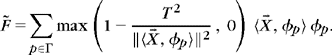
The matching pursuit algorithm in Section 12.3.1 is extended by searching for dictionary elements that maximize the norm of the multichannel inner product vector. We set the relaxation parameter α = 1. Let ![]() be a dictionary of unit vectors. The matching pursuit algorithm is initialized with
be a dictionary of unit vectors. The matching pursuit algorithm is initialized with ![]() . At each iteration m, it selects a best vector
. At each iteration m, it selects a best vector ![]() such that
such that
The orthogonal projection on this vector defines a new residue
with an energy conservation
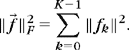
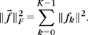
Theorem 12.6 thus remains valid by using the Frobenius norm over signal vectors, which proves the exponential convergence of the algorithm:

After M matching pursuit iterations, a back projection algorithm recovers the orthogonal projection of ![]() on the selected atoms {φpm}0 ≤ m < M. It can be computed with a Richardson gradient descent described afterwards for backprojecting an 11 pursuit, which is initialized with
on the selected atoms {φpm}0 ≤ m < M. It can be computed with a Richardson gradient descent described afterwards for backprojecting an 11 pursuit, which is initialized with ![]() .
.
The orthogonal matching pursuit of Section 12.3.2 is similarly extended. At a step m, a vector φpm is selected as in (12.158). A Gram-Schmidt orthogonalization decomposes φpm into its projection over the previously selected vectors {φpk}0 ≤ k < m plus an orthogonal complement um. The orthogonalized residue is then
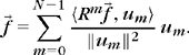
It decomposes ![]() over an orthogonal family {um}m and for signals of size N:
over an orthogonal family {um}m and for signals of size N:
The orthogonal matching pursuit properties thus remain essentially the same.
Multichannel l1 Pursuits
Sparse multichannel signal representations in redundant dictionaries can also be computed with l1 pursuits, which minimize an l1 norm of the coefficients. An l1 norm over multichannel vectors of coefficients is defined by
We denote
A sparse 11 pursuit approximation of a vector ![]() at a precision ε is defined by
at a precision ε is defined by ![]() with
with
A solution of this convex optimization is computed with an l1 Lagrangian minimization
where T depends on ε. Several authors have studied the approximation properties of l1 vector pursuits and their generalizations [157, 188, 462].
The l1 Lagrangian minimization (12.159) is numerically solved with the iterative thresholding algorithm of Section 12.4.3, which is adjusted as follows. We write ![]() .
.
1. Initialization. Choose ![]() , set k = 0, and compute
, set k = 0, and compute ![]() .
.
where ![]() .
.
where ![]() .
.
4. Stop. If ![]() is smaller than a fixed-tolerance criterion, stop the iterations; otherwise, set k ← k + 1 and go back to 2.
is smaller than a fixed-tolerance criterion, stop the iterations; otherwise, set k ← k + 1 and go back to 2.
If ![]() is the support of the computed solution after convergence, then like for a matching pursuit, a backprojection algorithm computes the orthogonal projection of
is the support of the computed solution after convergence, then like for a matching pursuit, a backprojection algorithm computes the orthogonal projection of ![]() on the selected atoms
on the selected atoms ![]() . It can be implemented with a Richardson gradient descent. It continues the gradient descent iterations of step 2, and replaces the soft thresholding in step 3 by a projector defined
. It can be implemented with a Richardson gradient descent. It continues the gradient descent iterations of step 2, and replaces the soft thresholding in step 3 by a projector defined ![]() if
if![]() and
and ![]() if
if![]() .
.
Multichannel Dictionaries
Multichannel signals ![]() have been decomposed over dictionaries of scalar signals {φp}p∈Γ, thus implying that the same dictionary elements {φp}p∈Λ are appropriate to approximate all signal channels (fk)0 ≤ k < K. More flexibility can be provided by dictionaries of multiple channel signals
have been decomposed over dictionaries of scalar signals {φp}p∈Γ, thus implying that the same dictionary elements {φp}p∈Λ are appropriate to approximate all signal channels (fk)0 ≤ k < K. More flexibility can be provided by dictionaries of multiple channel signals ![]() where each
where each ![]() includes K channels. In the context of color images, this means constructing a dictionary of color vectors having three color channels. Applying color dictionaries to color images can indeed improve the restitution of colors in noise-removal applications [357].
includes K channels. In the context of color images, this means constructing a dictionary of color vectors having three color channels. Applying color dictionaries to color images can indeed improve the restitution of colors in noise-removal applications [357].
Inner product vectors and projectors over dictionary vectors are written as
The thresholds and pursuit algorithms of Sections 12.6.1 and 12.6.2 decompose ![]() in a dictionary of scalar signals {φp}p∈Γ. They are directly extended to decompose
in a dictionary of scalar signals {φp}p∈Γ. They are directly extended to decompose ![]() in a dictionary of signal vectors
in a dictionary of signal vectors ![]() . In all formula and algorithms
. In all formula and algorithms
For a fixed index p, instead of decomposing all signal channels fk on the same φp, the resulting algorithms decompose each fk on a potentially different φp,k, but all channels make a simultaneous choice of a dictionary vector ![]() . Computations and mathematical properties are otherwise the same. The difficulty introduced by this flexibility is to construct dictionaries specifically adapted to each signal channel. Dictionary learning provides an approach to solve this issue.
. Computations and mathematical properties are otherwise the same. The difficulty introduced by this flexibility is to construct dictionaries specifically adapted to each signal channel. Dictionary learning provides an approach to solve this issue.
12.7 LEARNING DICTIONARIES
For a given dictionary size P, the dictionary should be optimized to best approximate signals in a given set ![]() . Prior information on signals can lead to appropriate dictionary design, for example, with Gabor functions, wavelets, or local cosine vectors. These dictionaries, however, can be optimized by better taking into account the signal properties derived from examples. Olshausen and Field [391] argue that such a learning process is part of biological evolution, and could explain how the visual pathway has been optimized to extract relevant information from visual scenes. Many open questions remain on dictionary learning, but numerical algorithms show that learning is possible and can improve applications.
. Prior information on signals can lead to appropriate dictionary design, for example, with Gabor functions, wavelets, or local cosine vectors. These dictionaries, however, can be optimized by better taking into account the signal properties derived from examples. Olshausen and Field [391] argue that such a learning process is part of biological evolution, and could explain how the visual pathway has been optimized to extract relevant information from visual scenes. Many open questions remain on dictionary learning, but numerical algorithms show that learning is possible and can improve applications.
Let us consider a family of K signal examples {fk}0 ≤ k < K. We want to find a dictionary ![]() of size |Γ| = P in which each fk has an “optimally” sparse approximation
of size |Γ| = P in which each fk has an “optimally” sparse approximation
given a precision ![]() . This sparse decomposition may be computed with a matching pursuit, an orthogonal matching pursuit, or an l1 pursuit. Let φfk = {〈fk, φp〉}p∈Γ be the dictionary operator with rows equal to the dictionary vectors φp. The learning process iteratively adjusts D to optimize the sparse representation of all examples.
. This sparse decomposition may be computed with a matching pursuit, an orthogonal matching pursuit, or an l1 pursuit. Let φfk = {〈fk, φp〉}p∈Γ be the dictionary operator with rows equal to the dictionary vectors φp. The learning process iteratively adjusts D to optimize the sparse representation of all examples.
Dictionary Update
Following the work of Olshausen and Field [391], several algorithms have been proposed to optimize ![]() , and thus φ, from a family of examples [78, 246, 336, 347]. It is a highly non-convex optimization problem that therefore can be trapped in local minima.
, and thus φ, from a family of examples [78, 246, 336, 347]. It is a highly non-convex optimization problem that therefore can be trapped in local minima.
The approach of Engan, Aase, and Husoy [246] performs alternate optimizations, similar to the Lloyd-Max algorithm for learning code books in vector quantization [27]. Let us write ![]() . Its Frobenius norm is
. Its Frobenius norm is
According to (12.162), the approximation vector ![]() can be written as
can be written as ![]() . The algorithm alternates between the calculation of the matrix of sparse signal coefficients A = (a[k,p])0 ≤ k < K,p∈Γ and a modification of the dictionary vectors φp to minimize the Frobenius norm of the residual error
. The algorithm alternates between the calculation of the matrix of sparse signal coefficients A = (a[k,p])0 ≤ k < K,p∈Γ and a modification of the dictionary vectors φp to minimize the Frobenius norm of the residual error
The matrix Φ can be considered as a vector transformed by the operator A. As explained in Section 5.1.3, the error ![]() is minimum if AΦ is the orthogonal projection of
is minimum if AΦ is the orthogonal projection of ![]() in the image space of A. It results that Φ is computed with the pseudo inverse A+ of A:
in the image space of A. It results that Φ is computed with the pseudo inverse A+ of A:
The inversion of the operator L = A*A can be implemented with the conjugate-gradient algorithm in Theorem 5.8. The resulting learning algorithm proceeds as follows:
1. Initialization. Each vector φp is initialized as a white Gaussian noise with a norm scaled to 1.
2. Sparse approximation. Calculation with a pursuit of the matrix A = (a[k,p])0≤k<K,p∈Γ of sparse approximation coefficients
3. Dictionary update. Minimization of the residual error (12.163) with
4. Dictionary normalization. Each resulting row Φp of Φ is normalized: ‖Φp‖ = 1.
5. Stopping criterion. After a fixed number of iterations, or if Φ is marginally modified, then stop; otherwise, go back to 2.
This algorithm is computationally very intensive since it includes a sparse approximation at each iteration and requires the inversion of the P × P matrix A*A. The sparse approximations are often calculated with an orthogonal pursuit that provides a good precision versus calculation trade-off. When the sparse coefficients a[k,p] are computed with an l1 pursuit, then one can prove that the algorithm converges to a stationary point [466].
To compress structured images such as identity photographs, Bryt and Elad showed that such learning algorithms are able to construct highly efficient dictionaries [123]. It is also used for video compression with matching pursuit by optimizing a predefined dictionary, which improves the distortion rate [426].
Translation-Invariant Dictionaries
For noise removal or inverse problems, the estimation of stationary signals is improved with translation-invariant dictionaries. As a result, the algorithm must only learn the P generators of this translation-invariant dictionary. A maximum support size for these dictionary vectors is set to a relatively small value of typically N = 16 × 16 pixels. The examples ![]() are then chosen to be small patches of N pixels, extracted from images.
are then chosen to be small patches of N pixels, extracted from images.
Optimized translation-invariant dictionaries lead to high-quality, state-of-the-art noise-removal results [242]. For color images, it can also incorporate intrinsic redundancy between the different color channels by learning color vectors [357]. Section 12.6 explains how to extend pursuit algorithms to multiple channel signals such as color images. Besides denoising, these dictionaries are used in super-resolution inverse problems—for example, to recover missing color pixels in high-resolution color demosaicing [357].
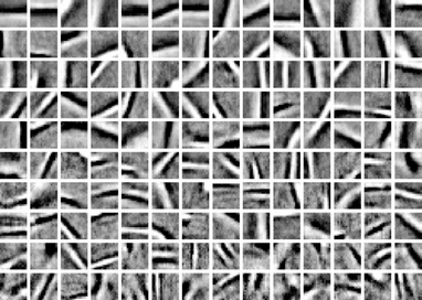
Figure 12.26 shows an example of a dictionary learned with this algorithm with N = 162 and P = 2N. The calculated dictionary vectors Φp look similar to the directional wavelets of Section 5.5. Olshausen and Field [391] observed that these dictionary vectors learned from natural images also look similar to the impulse response of simple cell neurons in the visual cortical area V1. It supports the idea of a biological adaptation to process visual scenes.
12.8 EXERCISES
12.1. 2 Best wavelet packet and local cosine approximations:
12.2. 3 Describe a coding algorithm that codes the position of M nonzero orthogonal coefficients in a best wavelet packet or local cosine dictionary tree of size P = N log2 N, and that requires less than ![]() bits. How many bits does your algorithm require?
bits. How many bits does your algorithm require?
12.3. 2 A double tree of block wavelet packet bases is defined in Exercise 8.12. Describe a fast best-basis algorithm that requires O(N(log2N)2) operations to find the block wavelet packet basis that minimizes an additive cost (12.34) [299].
12.4. 2 In a dictionary ![]() of orthonormal bases, we write a0[p] a vector of orthogonal coefficients with a support Λ0 corresponding to an orthonormal family
of orthonormal bases, we write a0[p] a vector of orthogonal coefficients with a support Λ0 corresponding to an orthonormal family ![]() . We want to minimize the l1 Lagrangian among orthogonal coefficients:
. We want to minimize the l1 Lagrangian among orthogonal coefficients:
12.5. 2 Prove that if we add a vector h to an orthonormal basis ![]() , we obtain a redundant dictionary with a mutual coherence that satisfies
, we obtain a redundant dictionary with a mutual coherence that satisfies ![]() .
.
12.6. 2 Let ![]() be a Gabor dictionary as defined in (12.77). Let Λ be an index set of two Gabor atoms in
be a Gabor dictionary as defined in (12.77). Let Λ be an index set of two Gabor atoms in ![]() .
.
12.7. 2 Let ![]() be a Dirac-Fourier dictionary.
be a Dirac-Fourier dictionary.
12.8. 3 Uncertainty principle [227]. We consider two orthogonal bases ![]() ,
, ![]() of
of ![]() .
.
12.9. 3 Cumulated coherence. Let D = {φp}p∈Γ be a dictionary with ‖φp‖ = 1. The cumulated mutual coherence of D is
Show that D spans l2 (Z) and that |〈φp, φp′〉| = β|p−p′|. Hint: Consider the case p > p′
12.10. 2Spark. Let D = {φp}p∈Γ be a dictionary with ‖φp‖ = 1. The spark of D, introduced in [229], is