
CHAPTER 7 Wavelet Bases
One can construct wavelets ψ such that the dilated and translated family
is an orthonormal basis of L2(![]() ). Behind this simple statement lie very different points of view that open a fruitful exchange between harmonic analysis and discrete signal processing.
). Behind this simple statement lie very different points of view that open a fruitful exchange between harmonic analysis and discrete signal processing.
Orthogonal wavelets dilated by 2j carry signal variations at the resolution 2−j. The construction of these bases can be related to multiresolution signal approximations. Following this link leads us to an unexpected equivalence between wavelet bases and conjugate mirror filters used in discrete multirate filter banks. These filter banks implement a fast orthogonal wavelet transform that requires only O(N) operations for signals of size N. The design of conjugate mirror filters also gives new classes of wavelet orthogonal bases including regular wavelets of compact support. In several dimensions, wavelet bases of L2(![]() d) are constructed with separable products of functions of one variable. Wavelet bases are also adapted to bounded domains and surfaces with lifting algorithms.
d) are constructed with separable products of functions of one variable. Wavelet bases are also adapted to bounded domains and surfaces with lifting algorithms.
7.1 ORTHOGONAL WAVELET BASES
Our search for orthogonal wavelets begins with multiresolution approximations. For f ∈ L2(![]() ), the partial sum of wavelet coefficients
), the partial sum of wavelet coefficients ![]() can indeed be interpreted as the difference between two approximations of f at the resolutions 2−j+1 and 2−j. Multiresolution approximations compute the approximation of signals at various resolutions with orthogonal projections on different spaces {Vj}j∈
can indeed be interpreted as the difference between two approximations of f at the resolutions 2−j+1 and 2−j. Multiresolution approximations compute the approximation of signals at various resolutions with orthogonal projections on different spaces {Vj}j∈![]() . Section 7.1.3 proves that multiresolution approximations are entirely characterized by a particular discrete filter that governs the loss of information across resolutions. These discrete filters provide a simple procedure for designing and synthesizing orthogonal wavelet bases.
. Section 7.1.3 proves that multiresolution approximations are entirely characterized by a particular discrete filter that governs the loss of information across resolutions. These discrete filters provide a simple procedure for designing and synthesizing orthogonal wavelet bases.
7.1.1 Multiresolution Approximations
Adapting the signal resolution allows one to process only the relevant details for a particular task. In computer vision, Burt and Adelson [126] introduced a multiresolution pyramid that can be used to process a low-resolution image first and then selectively increase the resolution when necessary. This section formalizes multiresolution approximations, which set the ground for the construction of orthogonal wavelets.
The approximation of a function f at a resolution 2−j is specified by a discrete grid of samples that provides local averages of f over neighborhoods of size proportional to 2j. Thus, a multiresolution approximation is composed of embedded grids of approximation. More formally, the approximation of a function at a resolution 2−j is defined as an orthogonal projection on a space Vj ⊂ L2 (![]() ). The space Vj regroups all possible approximations at the resolution 2−j. The orthogonal projection of f is the function fj ∈ Vj that minimizes ‖f – fj‖. The following definition, introduced by Mallat [362] and Meyer [44], specifies the mathematical properties of multiresolution spaces. To avoid confusion, let us emphasize that a scale parameter 2j is the inverse of the resolution 2−j.
). The space Vj regroups all possible approximations at the resolution 2−j. The orthogonal projection of f is the function fj ∈ Vj that minimizes ‖f – fj‖. The following definition, introduced by Mallat [362] and Meyer [44], specifies the mathematical properties of multiresolution spaces. To avoid confusion, let us emphasize that a scale parameter 2j is the inverse of the resolution 2−j.
Definition 7.1:
Multiresolutions. A sequence {Vj}j∈![]() of closed subspaces of L2(
of closed subspaces of L2(![]() ) is a multiresolution approximation if the following six properties are satisfied:
) is a multiresolution approximation if the following six properties are satisfied:
 (7.4)
(7.4) (7.5)
(7.5)and there exists θ such that {θ(t – n)}n∈![]() is a Riesz basis of V0.
is a Riesz basis of V0.
Let us give an intuitive explanation of these mathematical properties. Property (7.1) means that Vj is invariant by any translation proportional to the scale 2j. As we shall see later, this space can be assimilated to a uniform grid with intervals 2j, which characterizes the signal approximation at the resolution 2−j. The inclusion (7.2) is a causality property that proves that an approximation at a resolution 2−j contains all the necessary information to compute an approximation at a coarser resolution 2−j–1. Dilating functions in Vj by 2 enlarges the details by 2 and (7.3) guarantees that it defines an approximation at a coarser resolution 2−j–1. When the resolution 2−j goes to 0 (7.4) implies that we lose all the details of f and
On the other hand, when the resolution 2−j goes +∞, property (7.5) imposes that the signal approximation converges to the original signal:
When the resolution 2−j increases, the decay rate of the approximation error ![]() depends on the regularity of f. In Section 9.1.3 we relate this error to the uniform Lipschitz regularity of f.
depends on the regularity of f. In Section 9.1.3 we relate this error to the uniform Lipschitz regularity of f.
The existence of a Riesz basis {θ(t – n)}n∈![]() of V0 provides a discretization theorem as explained in Section 3.1.3. The function θ can be interpreted as a unit resolution cell; Section 5.1.1 gives the definition of a Riesz basis. It is a family of linearly independent functions such that there exist B ≥ A > 0, which satisfy
of V0 provides a discretization theorem as explained in Section 3.1.3. The function θ can be interpreted as a unit resolution cell; Section 5.1.1 gives the definition of a Riesz basis. It is a family of linearly independent functions such that there exist B ≥ A > 0, which satisfy
This energy equivalence guarantees that signal expansions over {θ(t – n)}n∈![]() are numerically stable. One may verify that the family
are numerically stable. One may verify that the family ![]() is a Riesz basis of Vj with the same Riesz bounds A and B at all scales 2j. Theorem 3.4 proves that {θ(t – n)}n∈
is a Riesz basis of Vj with the same Riesz bounds A and B at all scales 2j. Theorem 3.4 proves that {θ(t – n)}n∈![]() is a Riesz basis if and only if
is a Riesz basis if and only if
 (7.9)
(7.9)EXAMPLE 7.1 Piecewise Constant Approximations
A simple multiresolution approximation is composed of piecewise constant functions. Space Vj is the set of all ![]() such that g(t) is constant for t ∈ [n2j, (n + 1)2j) and n ∈
such that g(t) is constant for t ∈ [n2j, (n + 1)2j) and n ∈![]() . The approximation at a resolution 2−j of f is the closest piecewise constant function on intervals of size 2j. The resolution cell can be chosen to be the box window θ = 1[0,1). Clearly, Vj ⊂Vj−1, since functions constant on intervals of size 2j are also constant on intervals of size 2j−1. The verification of the other multiresolution properties is left to the reader. It is often desirable to construct approximations that are smooth functions, in which case piecewise constant functions are not appropriate.
. The approximation at a resolution 2−j of f is the closest piecewise constant function on intervals of size 2j. The resolution cell can be chosen to be the box window θ = 1[0,1). Clearly, Vj ⊂Vj−1, since functions constant on intervals of size 2j are also constant on intervals of size 2j−1. The verification of the other multiresolution properties is left to the reader. It is often desirable to construct approximations that are smooth functions, in which case piecewise constant functions are not appropriate.
EXAMPLE 7.2 Shannon Approximations
Frequency band-limited functions also yield multiresolution approximations. Space Vj is defined as the set of functions with a Fourier transform support included in [–2−jπ, 2−j π]. Theorem 3.5 provides an orthonormal basis {θ(t – n)}n∈![]() of V0 defined by
of V0 defined by
All other properties of multiresolution approximation are easily verified.
The approximation at the resolution 2−j of f ∈ L2(![]() ) is the function
) is the function ![]() that minimizes
that minimizes ![]() . It is proved in (3.12) that its Fourier transform is obtained with a frequency filtering:
. It is proved in (3.12) that its Fourier transform is obtained with a frequency filtering:
This Fourier transform is generally discontinuous at ±2−jπ, in which case ![]() decays like |t|−1 for large |t|, even though f might have a compact support.
decays like |t|−1 for large |t|, even though f might have a compact support.
EXAMPLE 7.3 Spline Approximations
Polynomial spline approximations construct smooth approximations with fast asymptotic decay. The space Vj of splines of degree m ≥ 0 is the set of functions that are m − 1 times continuously differentiable and equal to a polynomial of degree m on any interval [n2j, (n + 1)2j] for n ∈ ![]() . When m = 0, it is a piecewise constant multiresolution approximation. When m = 1, functions in Vj are piecewise linear and continuous.
. When m = 0, it is a piecewise constant multiresolution approximation. When m = 1, functions in Vj are piecewise linear and continuous.
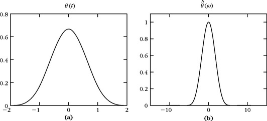
A Riesz basis of polynomial splines is constructed with box splines. A box spline θ of degree m is computed by convolving the box window 1[0, 1] with itself m + 1 times and centering at 0 or 1/2. Its Fourier transform is
If m is even, then ε = 1 and θ has a support centered at t = 1/2. If m is odd, then ε = 0 and θ(t) is symmetric about t = 0. Figure 7.1 displays a cubic box spline m = 3 and its Fourier transform. For all m ≥ 0, one can prove that {θ(t – n)}n∈![]() is a Riesz basis of V0 by verifying the condition (7.9). This is done with a closed-form expression for the series (7.19).
is a Riesz basis of V0 by verifying the condition (7.9). This is done with a closed-form expression for the series (7.19).
7.1.2 Scaling Function
The approximation of f at the resolution 2−j is defined as the orthogonal projection ![]() on Vj. To compute this projection, we must find an orthonormal basis of Vj. Theorem 7.1 orthogonalizes the Riesz basis {θ(t – n)}n∈
on Vj. To compute this projection, we must find an orthonormal basis of Vj. Theorem 7.1 orthogonalizes the Riesz basis {θ(t – n)}n∈![]() and constructs an orthogonal basis of each space Vj by dilating and translating a single function φ called a scaling function. To avoid confusing the resolution 2−j and the scale 2j, in the rest of this chapter the notion of resolution is dropped and
and constructs an orthogonal basis of each space Vj by dilating and translating a single function φ called a scaling function. To avoid confusing the resolution 2−j and the scale 2j, in the rest of this chapter the notion of resolution is dropped and ![]() is called an approximation at the scale 2j.
is called an approximation at the scale 2j.
Theorem 7.1.
Let {V}j∈![]() be a multiresolution approximation and φ be the scaling function having a Fourier transform
be a multiresolution approximation and φ be the scaling function having a Fourier transform
 (7.12)
The family {φj, n}n∈![]() is an orthonormal basis of Vj for all j ∈
is an orthonormal basis of Vj for all j ∈ ![]() .
.
Proof.
To construct an orthonormal basis, we look for a function φ ∈ V0. Thus, it can be expanded in the basis {θ(t – n)}n∈![]() :
:
where â is a 2π periodic Fourier series of finite energy. To compute â we express the orthogonality of {φ(t – n)}n∈![]() in the Fourier domain. Let
in the Fourier domain. Let ![]() . For any (n, p) ∈
. For any (n, p) ∈ ![]() 2,
2,
 (7.13)
Thus, {φ(t – n)}n∈![]() is orthonormal if and only if
is orthonormal if and only if ![]() . Computing the Fourier transform of this equality yields
. Computing the Fourier transform of this equality yields
 (7.14)
Indeed, the Fourier transform of ![]() is
is ![]() , and we proved in (33) that sampling a function periodizes its Fourier transform. The property (7.14) is verified if we choose
, and we proved in (33) that sampling a function periodizes its Fourier transform. The property (7.14) is verified if we choose

We saw in (7.9) that the denominator has a strictly positive lower bound, so â is a 2π periodic function of finite energy. ![]()
Approximation
The orthogonal projection of f over Vj is obtained with an expansion in the scaling orthogonal basis
provide a discrete approximation at the scale 2j. We can rewrite them as a convolution product:
with ![]() . The energy of the Fourier transform
. The energy of the Fourier transform ![]() is typically concentrated in [–π, π], as illustrated by Figure 7.2. As a consequence, the Fourier transform
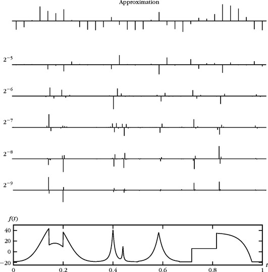
is typically concentrated in [–π, π], as illustrated by Figure 7.2. As a consequence, the Fourier transform ![]() is mostly nonnegligible in [–2−jπ, 2−jπ]. The discrete approximation aj[n] is therefore a low-pass filtering of f sampled at intervals 2j. Figure 7.3 gives a discrete multiresolution approximation at scales 2−9 ≤ 2j ≤ 2−4.
is mostly nonnegligible in [–2−jπ, 2−jπ]. The discrete approximation aj[n] is therefore a low-pass filtering of f sampled at intervals 2j. Figure 7.3 gives a discrete multiresolution approximation at scales 2−9 ≤ 2j ≤ 2−4.


EXAMPLE 7.5:
Spline multiresolution approximations admit a Riesz basis constructed with a box spline θ of degree m, having a Fourier transform given by (7.11). Inserting this expression in (7.12) yields
 (7.19)
and ε = 1 if m is even or ε = 0 if m is odd. A closed-form expression of S2m+2(ω) is obtained by computing the derivative of order 2m of the identity
The cubic spline–scaling function corresponds to m = 3, and ![]() is calculated with (7.18) by inserting
is calculated with (7.18) by inserting
 (7.22)
This cubic spline–scaling function φ and its Fourier transform are displayed in Figure 7.2. It has an infinite support but decays exponentially.
7.1.3 Conjugate Mirror Filters
A multiresolution approximation is entirely characterized by the scaling function φ that generates an orthogonal basis of each space Vj. We study the properties of φ, which guarantee that the spaces Vj satisfy all conditions of a multiresolution approximation. It is proved that any scaling function is specified by a discrete filter called a conjugate mirror filter.
Scaling Equation
The multiresolution causality property (7.2) imposes that Vj ⊂ Vj − 1; in particular, ![]() . Since
. Since ![]() is an orthonormal basis of V0, we can decompose
is an orthonormal basis of V0, we can decompose
This scaling equation relates a dilation of φ by 2 to its integer translations. The sequence h[n] will be interpreted as a discrete filter.
The Fourier transform of both sides of (7.23) yields
for ![]() . Thus, it is tempting to express
. Thus, it is tempting to express ![]() directly as a product of dilations of ĥ(ω). For any p ≥ 0, (7.25) implies
directly as a product of dilations of ĥ(ω). For any p ≥ 0, (7.25) implies
 (7.27)
If ![]() is continuous at ω = 0, then
is continuous at ω = 0, then ![]() so
so
 (7.28)
Theorem 7.2 [44, 362] gives necessary and sufficient conditions on ĥ(ω) to guarantee that this infinite product is the Fourier transform of a scaling function.
Theorem 7.2.
Mallat, Meyer. Let φ ∈ L2(![]() ) bean integrable scaling function. The Fourier series of h[n] = 〈2−1/2ϕ(t/2), ϕ(t – n)〉 satisfies
) bean integrable scaling function. The Fourier series of h[n] = 〈2−1/2ϕ(t/2), ϕ(t – n)〉 satisfies
Conversely, if ĥ(ω) is 2π periodic and continuously differentiable in a neighborhood of ω = 0, if it satisfies (7.29) and (7.30) and if
 (7.32)
Proof.
This theorem is a central result and its proof is long and technical. It is divided in several parts.
Proof of the necessary condition (7.29). The necessary condition is proved to be a consequence of the fact that ![]() is orthonormal. In the Fourier domain, (7.14) gives an equivalent condition:
is orthonormal. In the Fourier domain, (7.14) gives an equivalent condition:
 (7.33)
Since ĥ(ω) is 2π periodic, separating the even and odd integer terms gives

Inserting (7.33) for ω′ = ω/2 and ω′ = ω/2 + π proves that
Proof of the necessary condition(7.30). We prove that ĥ(0) = √2 by showing that ![]() . Indeed, we know that
. Indeed, we know that ![]() . More precisely, we verify that
. More precisely, we verify that ![]() is a consequence of the completeness property (7.5) of multiresolution approximations.
is a consequence of the completeness property (7.5) of multiresolution approximations.
The orthogonal projection of f ∈ L2(![]() ) on Vj is
) on Vj is
Property (7.5) expressed in the time and Fourier domains with the Plancherel formula implies that
To compute the Fourier transform ![]() , we denote
, we denote ![]() . Inserting the convolution expression (7.17) in (7.34) yields
. Inserting the convolution expression (7.17) in (7.34) yields
The Fourier transform of ![]() is
is ![]() . A uniform sampling has a periodized Fourier transform calculated in (33), and thus,
. A uniform sampling has a periodized Fourier transform calculated in (33), and thus,
 (7.36)
Let us choose ![]() . For j > 0 and ω ∈ [–π, π], (7.36) gives
. For j > 0 and ω ∈ [–π, π], (7.36) gives ![]() . The mean-square convergence (7.35) implies that
. The mean-square convergence (7.35) implies that
Since φ is integrable, ![]() is continuous and thus
is continuous and thus ![]()
We now prove that the function φ, having a Fourier transform given by (7.32), is a scaling function. This is divided in two intermediate results.
Proof that ![]() is orthonormal. Observe first that the infinite product (7.32) converges and that
is orthonormal. Observe first that the infinite product (7.32) converges and that ![]() because (7.29) implies that
because (7.29) implies that ![]() . The Parseval formula gives
. The Parseval formula gives
Verifying that ![]() is orthonormal is equivalent to showing that
is orthonormal is equivalent to showing that
This result is obtained by considering the functions

and computing the limit, as k increases to +∞, of the integrals
First, let us show that Ik[n] = 2πδ[n] for all k ≥ 1. To do this, we divide Ik[n] into two integrals:

Let us make the change of variable ω′ = ω + 2kπ in the first integral. Since ĥ(ω) is 2π periodic, when p < k, then ![]() . When k = p the hypothesis (7.29) implies that
. When k = p the hypothesis (7.29) implies that
For k > 1, the two integrals of Ik[n] become
 (7.37)
Since ![]() is 2kπ periodic we obtain Ik[n] = Ik–1 [n], and by induction Ik[n] = I1[n]. Writing (7.37) for k = 1 gives
is 2kπ periodic we obtain Ik[n] = Ik–1 [n], and by induction Ik[n] = I1[n]. Writing (7.37) for k = 1 gives
which verifies that Ik[n] = 2πδ[n], for all k ≥ 1.
We shall now prove that ![]() . For all ω ∈
. For all ω ∈ ![]() ,
,

The Fatou lemma (A.1) on positive functions proves that
because Ik[0] = 2π for all k ≥ 1. Since
by applying the dominated convergence theorem (A.1). This requires verifying the upper-bound condition (A.1). This is done in our case by proving the existence of a constant C such that
Indeed, we showed in (7.38) that ![]() is an integrable function.
is an integrable function.
The existence of C > 0 satisfying (7.40) is trivial for |ω| > 2kπ since ![]() . it follows that
. it follows that
Therefore, to prove (7.40) for |ω| ≤ 2kπ, it is sufficient to show that ![]() for ω ∈ [–π, π].
for ω ∈ [–π, π].
Let us first study the neighborhood of ω = 0. Since ĥ(ω) is continuously differentiable in this neighborhood and since |ĥ(ω)|2 ≤ 2 = |ĥ(0)|2, the functions |ĥ(ω)|2 and loge |ĥ(ω)|2 have derivatives that vanish at ω = 0. It follows that there exists ε > 0 such that
 (7.41)
Now let us analyze the domain |ω| > ε. To do this we take an integer l such that 2−l π < ε. Condition (7.31) proves that K = infω∈[–π/2, π/2] |ĥ(ω)| > 0, so if |ω| ≤ π,

This last result finishes the proof of inequality (7.40). Applying the dominated convergence theorem (A.1) proves (7.39) and that {φ(t – n)}n∈![]() is orthonormal. A simple change of variable shows that {φj,n}n∈
is orthonormal. A simple change of variable shows that {φj,n}n∈![]() is orthonormal for all j ∈
is orthonormal for all j ∈ ![]() .
.
Proof that {Vj}j∈![]() is a multiresolution approximation. To verify that φ is a scaling function, we must show that the spaces Vj generated by
is a multiresolution approximation. To verify that φ is a scaling function, we must show that the spaces Vj generated by ![]() define a multiresolution approximation. The multiresolution properties (7.1) and (7.3) are clearly true. The causality Vj+1 ⊂ Vj is verified by showing that for any p ∈
define a multiresolution approximation. The multiresolution properties (7.1) and (7.3) are clearly true. The causality Vj+1 ⊂ Vj is verified by showing that for any p ∈ ![]() ,
,
This equality is proved later in (7.107). Since all vectors of a basis of Vj+1 can be decomposed in a basis of Vj, it follows that Vj+1 ⊂ Vj.
To prove the multiresolution property (7.4) we must show that any f ∈ L2(R) satisfies
Since ![]() is an orthonormal basis of Vj,
is an orthonormal basis of Vj,
Suppose first that f is bounded by A and has a compact support included in [2J, 2J]. The constants A and J may be arbitrarily large. It follows that

Applying the Cauchy-Schwarz inequality to 1 × |φ(2−jt – n)| yields

with Sj = ∪n∈![]() [n − 2J–j, n + 2J–j] for j > J. For
[n − 2J–j, n + 2J–j] for j > J. For ![]() , we obviously have
, we obviously have ![]() 0 for j→ +∞. The dominated convergence theorem (A.1) applied to
0 for j→ +∞. The dominated convergence theorem (A.1) applied to ![]() proves that the integral converges to 0 and thus,
proves that the integral converges to 0 and thus,
Property (7.42) is extended to any f ∈ L2(![]() ) by using the density in L2(
) by using the density in L2(![]() ) of bounded function with a compact support, and Theorem A.5.
) of bounded function with a compact support, and Theorem A.5.
To prove the last multiresolution property (7.5) we must show that for any f ∈ L2(![]() ),
),
We consider functions f that have a Fourier transform ![]() that has a compact support included in [–2Jπ, 2Jπ] for J large enough. We proved in (7.36) that the Fourier transform of
that has a compact support included in [–2Jπ, 2Jπ] for J large enough. We proved in (7.36) that the Fourier transform of ![]() is
is

If j < –J, then the supports of ![]() are disjoint for different k, so
are disjoint for different k, so
 (7.44)
We have already observed that |φ(ω)| ≤ 1 and (7.41) proves that if ω is sufficiently small then |φ(ω)| ≥ e−|ω|, so
Since ![]() and
and ![]() , one can apply the dominated convergence theorem (A.1), to prove that
, one can apply the dominated convergence theorem (A.1), to prove that
The operator ![]() is an orthogonal projector, so
is an orthogonal projector, so ![]() . With (7.44) and (7.45), this implies that
. With (7.44) and (7.45), this implies that ![]() and thus verifies (7.43). This property is extended to any f ∈ L2(
and thus verifies (7.43). This property is extended to any f ∈ L2(![]() ) by using the density in L2(
) by using the density in L2(![]() ) of functions having compactly supported Fourier transforms and the result of Theorem A.5.
) of functions having compactly supported Fourier transforms and the result of Theorem A.5. ![]()
Discrete filters that have transfer functions that satisfy (7.29) are called conjugate mirror filters. As we shall see in Section 7.3, they play an important role in discrete signal processing; they make it possible to decompose discrete signals in separate frequency bands with filter banks. One difficulty of the proof is showing that the infinite cascade of convolutions that is represented in the Fourier domain by the product (7.32) does converge to a decent function in L2(![]() ). The sufficient condition (7.31) is not necessary to construct a scaling function, but it is always satisfied in practical designs of conjugate mirror filters. It cannot just be removed as shown by the example ĥ(ω) = cos(3ω/2), which satisfies all other conditions. In this case, a simple calculation shows that φ = 1/3 1[–3/2, 3/2]. Clearly {φ(t – n)}n∈
). The sufficient condition (7.31) is not necessary to construct a scaling function, but it is always satisfied in practical designs of conjugate mirror filters. It cannot just be removed as shown by the example ĥ(ω) = cos(3ω/2), which satisfies all other conditions. In this case, a simple calculation shows that φ = 1/3 1[–3/2, 3/2]. Clearly {φ(t – n)}n∈![]() is not orthogonal, so φ is not a scaling function. However, the condition (7.31) may be replaced by a weaker but more technical necessary and sufficient condition proved by Cohen [16, 167].
is not orthogonal, so φ is not a scaling function. However, the condition (7.31) may be replaced by a weaker but more technical necessary and sufficient condition proved by Cohen [16, 167].
EXAMPLE 7.8
Polynomial splines of degree m correspond to a conjugate mirror filter ĥ(ω) that is calculated from ![]() with (7.25):
with (7.25):
Inserting (7.18) yields
 (7.48)
where ε = 0 if m is odd and ε = 1 if m is even. For linear splines m = 1, so (7.20) implies that
For cubic splines, the conjugate mirror filter is calculated by inserting (7.22) in (7.48). Figure 7.4 gives the graph of |ĥ(ω)|2. The impulse responses h[n] of these filters have an infinite support but an exponential decay. For m odd, h[n] is symmetric about n = 0. Table 7.1 gives the coefficients h[n] above 10−4 for m = 1, 3.
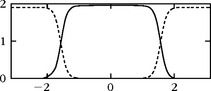
FIGURE 7.4 The solid line gives |ĥ(ω)|2 on [–π, π] for a cubic spline multiresolution. The dotted line corresponds to ![]() .
.
Table 7.1 Conjugate Mirror Filters h[n] for Linear Splines m = 1 and Cubic Splines m = 3
| n | h[n] | |
|---|---|---|
| m = 1 | 0 | 0.817645956 |
| 1, −1 | 0.397296430 | |
| 2, −2 | −0.069101020 | |
| 3, −3 | −0.051945337 | |
| 4, −4 | 0.016974805 | |
| 5, −5 | 0.009990599 | |
| 6, −6 | −0.003883261 | |
| 7, −7 | −0.002201945 | |
| 8, −8 | 0.000923371 | |
| 9, −9 | 0.000511636 | |
| 10, −10 | −0.000224296 | |
| 11, −11 | −0.000122686 | |
| m = 3 | 0 | 0.766130398 |
| 1, −1 | 0.433923147 | |
| 2, −2 | −0.050201753 | |
| 3, −3 | −0.110036987 | |
| 4, −4 | 0.032080869 | |
| m = 3 | 5, −5 | 0.042068328 |
| 6, −6 | −0.017176331 | |
| 7, −7 | −0.017982291 | |
| 8, −8 | 0.008685294 | |
| 9, −9 | 0.008201477 | |
| 10, −10 | −0.004353840 | |
| 11, −11 | −0.003882426 | |
| 12, −12 | 0.002186714 | |
| 13, −13 | 0.001882120 | |
| 14, −14 | −0.001103748 | |
| 15, −15 | −0.000927187 | |
| 16, −16 | 0.000559952 | |
| 17, −17 | 0.000462093 | |
| 18, −18 | −0.000285414 | |
| 19, −19 | −0.000232304 | |
| 20, −20 | 0.000146098 |
Note: The coefficients below 10−4 are not given.
7.1.4 In Which Orthogonal Wavelets Finally Arrive
Orthonormal wavelets carry the details necessary to increase the resolution of a signal approximation. The approximations of f at the scales 2j and 2j–1 are, respectively, equal to their orthogonal projections on Vj and Vj–1. We know that Vj is included in Vj–1. Let Wj be the orthogonal complement of Vj in Vj–1:
The orthogonal projection of f on Vj–1 can be decomposed as the sum of orthogonal projections on Vj and Wj:
The complement ![]() provides the “details” of f that appear at the scale 2j–1 but that disappear at the coarser scale 2j Theorem 7.3 [44, 362] proves that one can construct an orthonormal basis of Wj by scaling and translating a wavelet ψ.
provides the “details” of f that appear at the scale 2j–1 but that disappear at the coarser scale 2j Theorem 7.3 [44, 362] proves that one can construct an orthonormal basis of Wj by scaling and translating a wavelet ψ.
Theorem 7.3.
Mallat, Meyer. Let φ be a scaling function and h the corresponding conjugate mirror filter. Let ψ be the function having a Fourier transform
For any scale 2j, {ψj,n}n∈![]() is an orthonormal basis of Wj. For all scales,
is an orthonormal basis of Wj. For all scales, ![]() is an orthonormal basis of L2(
is an orthonormal basis of L2(![]() ).
).
Proof.
Let us prove first that ![]() can be written as the product (7.52). Necessarily, ψ(t/2) ∈ W1 ⊂ V0. Thus, it can be decomposed in {φ(t – n)}n∈
can be written as the product (7.52). Necessarily, ψ(t/2) ∈ W1 ⊂ V0. Thus, it can be decomposed in {φ(t – n)}n∈![]() , which is an orthogonal basis of V0:
, which is an orthogonal basis of V0:
The Fourier transform of (7.54) yields
Lemma 7.1 gives necessary and sufficient conditions on ![]() for designing an orthogonal wavelet.
for designing an orthogonal wavelet.
Lemma 7.1.
The family {ψj,n}n∈![]() is an orthonormal basis of Wj if and only if
is an orthonormal basis of Wj if and only if
The lemma is proved for j = 0 from which it is easily extended to j ≠ 0 with an appropriate scaling. As in (7.14), one can verify that {ψ(t – n)}n∈![]() is orthonormal if and only if
is orthonormal if and only if
 (7.59)
We know that ![]() , so (7.59) is equivalent to (7.57).
, so (7.59) is equivalent to (7.57).
The space W0 is orthogonal to V0 if and only if {ϕ(t – n)}n∈![]() and {ψ(t – n)}n∈
and {ψ(t – n)}n∈![]() are orthogonal families of vectors. This means that for any n ∈
are orthogonal families of vectors. This means that for any n ∈ ![]() ,
,
The Fourier transform of ![]() . The sampled sequence
. The sampled sequence ![]() is zero if its Fourier series computed with (33) satisfies
is zero if its Fourier series computed with (33) satisfies
 (7.60)
By inserting ![]() and
and ![]() in this equation, since
in this equation, since ![]() , we prove as before that (7.60) is equivalent to (7.58).
, we prove as before that (7.60) is equivalent to (7.58).
We must finally verify that V–1 = V0 + W0. Knowing that {√2ϕ(2t – n)}n∈![]() is an orthogonal basis of V–1, it is equivalent to show that for any a[n] ∈
is an orthogonal basis of V–1, it is equivalent to show that for any a[n] ∈ ![]() 2(
2(![]() ) there exist b[n] ∈
) there exist b[n] ∈ ![]() 2(
2(![]() ) and c[n] ∈
) and c[n] ∈ ![]() 2(
2(![]() ) such that
) such that
This is done by relating ![]() and
and ![]() to â(ω). The Fourier transform of (7.61) yields
to â(ω). The Fourier transform of (7.61) yields
Inserting ![]() and
and ![]() in this equation shows that it is necessarily satisfied if
in this equation shows that it is necessarily satisfied if
When calculating the right side of (7.62), we verify that it is equal to the left side by inserting (7.57), (7.58), and using
Since ![]() and
and ![]() are 2π periodic they are the Fourier series of two sequences b[n] and c[n] that satisfy (7.61). This finishes the proof of the lemma.
are 2π periodic they are the Fourier series of two sequences b[n] and c[n] that satisfy (7.61). This finishes the proof of the lemma.
The formula (7.53)
satisfies (7.57) and (7.58) because of (7.63). Thus, we derive from Lemma 7.1 that ![]() is an orthogonal basis of Wj.
is an orthogonal basis of Wj.
We complete the proof of the theorem by verifying that ![]() is an orthogonal basis of L2(
is an orthogonal basis of L2(![]() ). Observe first that the detail spaces {Wj}j∈
). Observe first that the detail spaces {Wj}j∈![]() are orthogonal. Indeed, Wj is orthogonal to Vj and Wl ⊂ Vl–1 ⊂ Vj for j < l. Thus, Wj and Wl are orthogonal. We can also decompose
are orthogonal. Indeed, Wj is orthogonal to Vj and Wl ⊂ Vl–1 ⊂ Vj for j < l. Thus, Wj and Wl are orthogonal. We can also decompose
Indeed, Vj–1 = Wj ⊕ Vj, and we verify by substitution that for any L > J,
Since {Vj}j∈![]() is a multiresolution approximation, VL and VJ tend, respectively, to L2(
is a multiresolution approximation, VL and VJ tend, respectively, to L2(![]() ) and {0} when L and J go, respectively, to –∞ and +∞, which implies (7.64). Therefore, a union of orthonormal bases of all Wj is an orthonormal basis of L2(
) and {0} when L and J go, respectively, to –∞ and +∞, which implies (7.64). Therefore, a union of orthonormal bases of all Wj is an orthonormal basis of L2(![]() ).
).
The proof of the theorem shows that g is the Fourier series of
which are the decomposition coefficients of
Calculating the inverse Fourier transform of (7.53) yields
This mirror filter plays an important role in the fast wavelet transform algorithm.
EXAMPLE 7.9
Figure 7.5 displays the cubic spline wavelet ψ and its Fourier transform ψ calculated by inserting in (7.52) the expressions (7.18) and (7.48) of ![]() and ĥ(ω). The properties of this Battle-Lemarié spline wavelet are further studied in Section 7.2.2. Like most orthogonal wavelets, the energy of
and ĥ(ω). The properties of this Battle-Lemarié spline wavelet are further studied in Section 7.2.2. Like most orthogonal wavelets, the energy of ![]() is essentially concentrated in [–2π, –π] ∪ [π, 2π]. For any ψ that generates an orthogonal basis of L2(
is essentially concentrated in [–2π, –π] ∪ [π, 2π]. For any ψ that generates an orthogonal basis of L2(![]() ), one can verify that
), one can verify that
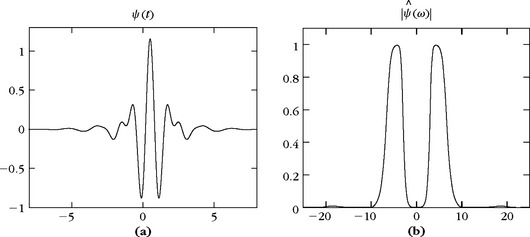

This is illustrated in Figure 7.6.

The orthogonal projection of a signal f in a “detail” space Wj is obtained with a partial expansion in its wavelet basis:
Thus, a signal expansion in a wavelet orthogonal basis can be viewed as an aggregation of details at all scales 2j that go from 0 to +∞:

Figure 7.7 gives the coefficients of a signal decomposed in the cubic spline wavelet orthogonal basis. The calculations are performed with the fast wavelet transform algorithm of Section 7.3. The up or down Diracs give the amplitudes of positive or negative wavelet coefficients at a distance 2j n at each scale 2j. Coefficients are nearly zero at fine scales where the signal is locally regular.
Wavelet Design
Theorem 7.3 constructs a wavelet orthonormal basis from any conjugate mirror filter ĥ(ω). This gives a simple procedure for designing and building wavelet orthogonal bases. Conversely, we may wonder whether all wavelet orthonormal bases are associated to a multiresolution approximation and a conjugate mirror filter. If we impose that ψ has a compact support, then Lemarié [52] proved that ψ necessarily corresponds to a multiresolution approximation. It is possible, however, to construct pathological wavelets that decay like |t|−1 at infinity, and that cannot be derived from any multiresolution approximation. Section 7.2 describes important classes of wavelet bases and explains how to design ĥ to specify the support, the number of vanishing moments, and the regularity of ψ.
7.2 CLASSES OF WAVELET BASES
7.2.1 Choosing a Wavelet
Most applications of wavelet bases exploit their ability to efficiently approximate particular classes of functions with few nonzero wavelet coefficients. This is true not only for data compression but also for noise removal and fast calculations. Therefore, the design of ψ must be optimized to produce a maximum number of wavelet coefficients 〈f, ψj, n〉 that are close to zero. A function f has few nonnegligible wavelet coefficients if most of the fine-scale (high-resolution) wavelet coefficients are small. This depends mostly on the regularity of f, the number of vanishing moments of ψ, and the size of its support. To construct an appropriate wavelet from a conjugate mirror filter h[n], we relate these properties to conditions on ĥ(ω).
Vanishing Moments
Let us recall that ψ has p vanishing moments if
This means that ψ is orthogonal to any polynomial of degree p − 1. Section 6.1.3 proves that if f is regular and ψ has enough vanishing moments, then the wavelet coefficients |〈f, ψj,n〉| are small at fine scales 2j. Indeed, if f is locally Ck, then over a small interval it is well approximated by a Taylor polynomial of degree k. If k < p, then wavelets are orthogonal to this Taylor polynomial, and thus produce small-amplitude coefficients at fine scales. Theorem 7.4 relates the number of vanishing moments of ψ to the vanishing derivatives of ![]() at ω = 0 and to the number of zeroes of ĥ(ω) at ω = π. It also proves that polynomials of degree p − 1 are then reproduced by the scaling functions.
at ω = 0 and to the number of zeroes of ĥ(ω) at ω = π. It also proves that polynomials of degree p − 1 are then reproduced by the scaling functions.
Theorem 7.4:
Vanishing Moments. Let ψ and ϕ be a wavelet and a scaling function that generate an orthogonal basis. Suppose that ![]() and
and ![]() . The four following statements are equivalent:
. The four following statements are equivalent:
Proof.
The decay of |φ(t)| and |ψ(t)| implies that ![]() and
and ![]() (ω) are p times continuously differentiable. The kth-order derivative
(ω) are p times continuously differentiable. The kth-order derivative ![]() is the Fourier transform of (–it)k ψ(t). Thus,
is the Fourier transform of (–it)k ψ(t). Thus,
We derive that (1) is equivalent to (2).
Theorem 7.3 proves that
Since ![]() , by differentiating this expression we prove that (2) is equivalent to (3).
, by differentiating this expression we prove that (2) is equivalent to (3).
Let us now prove that (4) implies (1). Since ψ is orthogonal to {φ(t – n)}n∈![]() , it is also orthogonal to the polynomials qk for 0 ≤ k < p. This family of polynomials is a basis of the space of polynomials of degree at most p − 1. Thus, ψ is orthogonal to any polynomial of degree p − 1 and in particular to tk for 0 ≤ k < p. This means that ψ has p vanishing moments.
, it is also orthogonal to the polynomials qk for 0 ≤ k < p. This family of polynomials is a basis of the space of polynomials of degree at most p − 1. Thus, ψ is orthogonal to any polynomial of degree p − 1 and in particular to tk for 0 ≤ k < p. This means that ψ has p vanishing moments.
To verify that (1) implies (4) we suppose that ψ has p vanishing moments, and for k < p, we evaluate qk(t) defined in (7.70). This is done by computing its Fourier transform:
Let δ(k) be the distribution that is the kth-order derivative of a Dirac, defined in Section A.7 in the Appendix. The Poisson formula (2.4) proves that
 (7.71)
With several integrations by parts, we verify the distribution equality
 (7.72)
where akm,l is a linear combination of the derivatives ![]() .
.
For l ≠ 0, let us prove that akm,l = 0 by showing that ![]() if 0 ≤ m < p. For any P > 0, (7.27) implies
if 0 ≤ m < p. For any P > 0, (7.27) implies
 (7.73)
Since ψ has p vanishing moments, we showed in (3) that ĥ(ω) has a zero of order p at ω = ±π. But ĥ(ω) is also 2π periodic, so (7.73) implies that ![]() in the neighborhood of ω = 2lπ, for any l ≠ 0. Thus,
in the neighborhood of ω = 2lπ, for any l ≠ 0. Thus, ![]()
Since akm,l = 0 and φ(2lπ) = 0 when l ≠ 0, it follows from (7.72) that
The only term that remains in the summation (7.71) is l = 0, and inserting (7.72) yields
The inverse Fourier transform of δ(m)(ω) is (2π)−1(– it)m, and Theorem 7.2 proves that ![]() . Thus, the inverse Fourier transform qk of
. Thus, the inverse Fourier transform qk of ![]() is a polynomial of degree k.
is a polynomial of degree k.
The hypothesis (4) is called the Fix-Strang condition [446]. The polynomials {qk}0≤k<p define a basis of the space of polynomials of degree p − 1. The Fix-Strang condition proves that ψ has p vanishing moments if and only if any polynomial of degree p − 1 can be written as a linear expansion of {ϕ(t – n)}n∈![]() . The decomposition coefficients of the polynomials qk do not have a finite energy because polynomials do not have a finite energy.
. The decomposition coefficients of the polynomials qk do not have a finite energy because polynomials do not have a finite energy.
Size of Support
If f has an isolated singularity at t0 and if t0 is inside the support of ![]() , then 〈f, ψj,n〉 may have a large amplitude. If ψ has a compact support of size K, at each scale 2j there are K wavelets ψj,n with a support including t0. To minimize the number of high-amplitude coefficients we must reduce the support size of ψ. Theorem 7.5 relates the support size of h to the support of φ and ψ.
, then 〈f, ψj,n〉 may have a large amplitude. If ψ has a compact support of size K, at each scale 2j there are K wavelets ψj,n with a support including t0. To minimize the number of high-amplitude coefficients we must reduce the support size of ψ. Theorem 7.5 relates the support size of h to the support of φ and ψ.
Theorem 7.5.
Compact Support. The scaling function φ has a compact support if and only if h has a compact support and their supports are equal. If the support of h and φ is [N1, N2], then the support of ψ is [(N1 – N2 + 1)/2, (N2 – N1 + 1)/2].
Proof.
If φ has a compact support, since
we derive that h also has a compact support. Conversely, the scaling function satisfies
If h has a compact support then one can prove [194] that ϕ has a compact support. The proof is not reproduced here.
To relate the support of ϕ and h, we suppose that h[n] is nonzero for N1 ≤ n ≤ N2 and that ϕ has a compact support [K1, K2]. The support of ϕ(t/2) is [2K1, 2K2]. The sum at the right of (7.74) is a function with a support of [N1 + K1, N2 + K2]. The equality proves that the support of ϕ is [K1, K2] = [N1, N2].
Let us recall from (7.68) and (7.67) that
If the supports of ϕ and h are equal to [N1, N2], the sum on the right side has a support equal to [N1 – N2 + 1, N2 – N1 + 1]. Thus, ψ has a support equal to [(N1 – N2 + 1)/2, (N2 – N1 + 1)/2].
If h has a finite impulse response in [N1, N2], Theorem 7.5 proves that ψ has a support of size N2 – N1 centered at 1/2. To minimize the size of the support, we must synthesize conjugate mirror filters with as few nonzero coefficients as possible.
Support versus Moments
The support size of a function and the number of vanishing moments are a priori independent. However, we shall see in Theorem 7.7 that the constraints imposed on orthogonal wavelets imply that if ψ has p vanishing moments, then its support is at least of size 2p − 1. Daubechies wavelets are optimal in the sense that they have a minimum size support for a given number of vanishing moments. When choosing a particular wavelet, we face a trade-off between the number of vanishing moments and the support size. If f has few isolated singularities and is very regular between singularities, we must choose a wavelet with many vanishing moments to produce a large number of small wavelet coefficients 〈f, ψj,n〉. If the density of singularities increases, it might be better to decrease the size of its support at the cost of reducing the number of vanishing moments. Indeed, wavelets that overlap the singularities create high-amplitude coefficients.
The multiwavelet construction of Geronimo, Hardin, and Massupust [271] offers more design flexibility by introducing several scaling functions and wavelets. Exercise 7.16 gives an example. Better trade-off can be obtained between the multiwavelets supports and their vanishing moments [447]. However, multiwavelet decompositions are implemented with a slightly more complicated filter bank algorithm than a standard orthogonal wavelet transform.
Regularity
The regularity of ψ has mostly a cosmetic influence on the error introduced by thresholding or quantizing the wavelet coefficients. When reconstructing a signal from its wavelet coefficients

an error ε added to a coefficient 〈f, Ψj,n〉 will add the wavelet component ε ψj,n to the reconstructed signal. If ψ is smooth, then εψj,n is a smooth error. For image-coding applications, a smooth error is often less visible than an irregular error, even though they have the same energy. Better-quality images are obtained with wavelets that are continuously differentiable than with the discontinuous Haar wavelet. Theorem 7.6 due to Tchamitchian [454] relates the uniform Lipschitz regularity of ϕ and ψ to the number of zeroes of ĥ(ω) at ω = π.
Theorem 7.6.
Tchamitchian. Let ĥ(ω) be a conjugate mirror filter with p zeroes at π and that satisfies the sufficient conditions of Theorem 7.2. Let us perform the factorization
If ![]() , then ψ and ϕ are uniformly Lipschitz α for
, then ψ and ϕ are uniformly Lipschitz α for
Proof.
This result is proved by showing that there exist C1 > 0 and C2 > 0 such that for all ω ∈ ![]()
The Lipschitz regularity of ϕ and ψ is then derived from Theorem 6.1, which shows that if ![]() , then f is uniformly Lipschitz α.
, then f is uniformly Lipschitz α.
We proved in (7.32) that ![]() . One can verify that
. One can verify that
 (7.78)
Let us now compute an upper bound for ![]() . At ω = 0, we have ĥ(0) = √2 so
. At ω = 0, we have ĥ(0) = √2 so ![]() . Since ĥ(ω) is continuously differentiable at ω = 0,
. Since ĥ(ω) is continuously differentiable at ω = 0, ![]() is also continuously differentiable at ω = 0. Thus, we derive that there exists ε > 0 such that if |ω| < ε, then
is also continuously differentiable at ω = 0. Thus, we derive that there exists ε > 0 such that if |ω| < ε, then ![]() . Consequently,
. Consequently,
 (7.79)
If |ω| > ε, there exists J ≥ 1 such that 2J–1 ε ≤ |ω| ≤ 2J ε, and we decompose
 (7.80)
Since ![]() , inserting (7.79) yields for |ω| > ε
, inserting (7.79) yields for |ω| > ε
 (7.81)
Since 2J ≤ ε−1 2|ω|, this proves that

Equation (7.76) is derived from (7.78) and this last inequality. Since ![]() , (7.77) is obtained from (7.76).
, (7.77) is obtained from (7.76).
This theorem proves that if B < 2p–1, then α0 > 0. It means that ϕ and ψ are uniformly continuous. For any m > 0, if B < 2p–1–m, then α0 > m, so ψ and ϕ are m times continuously differentiable. Theorem 7.4 shows that the number p of zeros of ĥ(ω) at π is equal to the number of vanishing moments of ψ. A priori, we are not guaranteed that increasing p will improve the wavelet regularity since B might increase as well. However, for important families of conjugate mirror filters such as splines or Daubechies filters, B increases more slowly than p, which implies that wavelet regularity increases with the number of vanishing moments. Let us emphasize that the number of vanishing moments and the regularity of orthogonal wavelets are related but it is the number of vanishing moments and not the regularity that affects the amplitude of the wavelet coefficients at fine scales.
7.2.2 Shannon, Meyer, Haar, and Battle-Lemarié Wavelets
We study important classes of wavelets with Fourier transforms that are derived from the general formula proved in Theorem 7.3,
Shannon Wavelet
The Shannon wavelet is constructed from the Shannon multiresolution approximation, which approximates functions by their restriction to low-frequency intervals. It corresponds to ![]() and
and ![]() for ω ∈ [–π, π]. We derive from (7.82) that
for ω ∈ [–π, π]. We derive from (7.82) that
This wavelet is C∞ but has a slow asymptotic time decay. Since ![]() is zero in the neighborhood of ω = 0, all its derivatives are zero at ω = 0. Thus, Theorem 7.4 implies that ψ has an infinite number of vanishing moments.
is zero in the neighborhood of ω = 0, all its derivatives are zero at ω = 0. Thus, Theorem 7.4 implies that ψ has an infinite number of vanishing moments.
Since ![]() has a compact support we know that ψ(t) is C∞. However, |ψ(t)| decays only like |t|−1 at infinity because
has a compact support we know that ψ(t) is C∞. However, |ψ(t)| decays only like |t|−1 at infinity because ![]() is discontinuous at ± π and ± 2π.
is discontinuous at ± π and ± 2π.
Meyer Wavelets
A Meyer wavelet [375] is a frequency band-limited function that has a Fourier transform that is smooth, unlike the Fourier transform of the Shannon wavelet. This smoothness provides a much faster asymptotic decay in time. These wavelets are constructed with conjugate mirror filters ĥ(ω) that are Cn and satisfy
The only degree of freedom is the behavior of ĥ(ω) in the transition bands [–2π/3, –π/3] ∪ [π/3, 2π/3]. It must satisfy the quadrature condition
and to obtain Cn junctions at |ω| = π/3 and |ω| = 2π/3, the n first derivatives must vanish at these abscissa. One can construct such functions that are C∞.
The scaling function ![]() has a compact support and one can verify that
has a compact support and one can verify that
 (7.86)
The resulting wavelet (7.82) is
 (7.87)
The functions ϕ and ψ are C∞ because their Fourier transforms have a compact support. Since ![]() in the neighborhood of ω = 0, all its derivatives are zero at ω = 0, which proves that ψ has an infinite number of vanishing moments.
in the neighborhood of ω = 0, all its derivatives are zero at ω = 0, which proves that ψ has an infinite number of vanishing moments.
If ĥ is Cn, then ![]() and
and ![]() are also Cn.The discontinuities of the (n + 1)th derivative of ĥ are generally at the junction of the transition band |ω| = π/3, 2π/3, in which case one can show that there exists A such that
are also Cn.The discontinuities of the (n + 1)th derivative of ĥ are generally at the junction of the transition band |ω| = π/3, 2π/3, in which case one can show that there exists A such that
Although the asymptotic decay of ψ is fast when n is large, its effective numerical decay may be relatively slow, which is reflected by the fact that A is quite large. As a consequence, a Meyer wavelet transform is generally implemented in the Fourier domain. Section 8.4.2 relates these wavelet bases to lapped orthogonal transforms applied in the Fourier domain. One can prove [19] that there exists no orthogonal wavelet that is C∞ and has an exponential decay.
EXAMPLE 7.10
To satisfy the quadrature condition (7.85), one can verify that ĥ in (7.84) may be defined on the transition bands by
where β(x) is a function that goes from 0 to 1 on the interval [0, 1] and satisfies
An example due to Daubechies [19] is
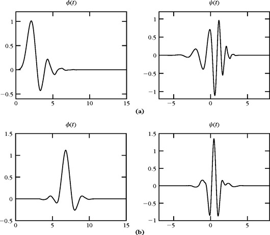
The resulting ĥ(ω) has n = 3 vanishing derivatives at |ω| = π/3, 2π/3. Figure 7.8 displays the corresponding wavelet ψ.

Haar Wavelets
The Haar basis is obtained with a multiresolution of piecewise constant functions. The scaling function is ϕ= 1[0, 1]. The filter h[n] given in (7.46) has two nonzero coefficients equal to 2−1/2 at n = 0 and n = 1. Thus,
 (7.90)
The Haar wavelet has the shortest support among all orthogonal wavelets. It is not well adapted to approximating smooth functions because it has only one vanishing moment.
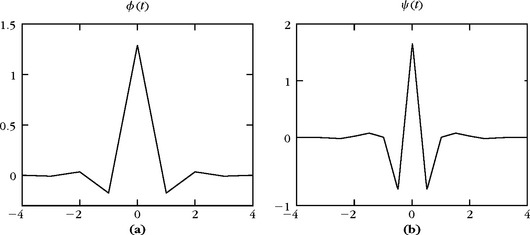
Battle-Lemarié Wavelets
Polynomial spline wavelets introduced by Battle [99] and Lemarié [345] are computed from spline multiresolution approximations. The expressions of ![]() and ĥ(ω) are given, respectively, by (7.18) and (7.48). For splines of degree m, ĥ(ω) and its first m derivatives are zero at ω = π. Theorem 7.4 derives that ψ has m + 1 vanishing moments. It follows from (7.82) that
and ĥ(ω) are given, respectively, by (7.18) and (7.48). For splines of degree m, ĥ(ω) and its first m derivatives are zero at ω = π. Theorem 7.4 derives that ψ has m + 1 vanishing moments. It follows from (7.82) that

This wavelet ψ has an exponential decay. Since it is a polynomial spline of degree m, it is m − 1 times continuously differentiable. Polynomial spline wavelets are less regular than Meyer wavelets but have faster time asymptotic decay. For m odd, ψ is symmetric about 1/2. For m even, it is antisymmetric about 1/2. Figure 7.5 gives the graph of the cubic spline wavelet ψ corresponding to m = 3. For m = 1, Figure 7.9 displays linear splines ϕ and ψ. The properties of these wavelets are further studied in [15, 106, 164].
7.2.3 Daubechies Compactly Supported Wavelets
Daubechies wavelets have a support of minimum size for any given number p of vanishing moments. Theorem 7.5 proves that wavelets of compact support are computed with finite impulse-response conjugate mirror filters h. We consider real causal filters h[n], which implies that ĥ is a trigonometric polynomial:
To ensure that ψ has p vanishing moments, Theorem 7.4 shows that ![]() must have a zero of order p at ω = π. To construct a trigonometric polynomial of minimal size, we factor (1 + e−iw)p, which is a minimum-size polynomial having p zeros at ω = π:
must have a zero of order p at ω = π. To construct a trigonometric polynomial of minimal size, we factor (1 + e−iw)p, which is a minimum-size polynomial having p zeros at ω = π:
The difficulty is to design a polynomial R(e −iw) of minimum degree m such that ĥ satisfies
As a result, h has N = m + p + 1 nonzero coefficients. Theorem 7.7 by Daubechies [194] proves that the minimum degree of R is m = p − 1.
Theorem 7.7.
Daubechies. A real conjugate mirror filter h, such that ĥ(ω) has p zeroes at ω = π, has at least 2p nonzero coefficients. Daubechies filters have 2p nonzero coefficients.
Proof.
The proof is constructive and computes Daubechies filters. Since h[n] is real, |ĥ(ω)|2 is an even function and can be written as a polynomial in cos ω. Thus, |R(e −iw)|2 defined in (7.91) is a polynomial in cos ω that we can also write as a polynomial P(sin2 (ω/2)),
The quadrature condition (7.92) is equivalent to
for any y = sin2(ω/2) ∈[0, 1]. To minimize the number of nonzero terms of the finite Fourier series ĥ(ω), we must find the solution P(y) ≥ 0 of minimum degree, which is obtained with the Bezout theorem on polynomials.
Theorem 7.8.
Bezout. Let Q1(y) and Q2(y) be two polynomials of degrees n1 and n2 with no common zeroes. There exist two unique polynomials P1(y) and P2(y) of degrees n2 − 1 and n1 − 1 such that
The proof of this classical result is in [19]. Since Q1(y) = (1 – y)p and Q2(y) = yp are two polynomials of degree p with no common zeros, the Bezout theorem proves that there exist two unique polynomials P1 (y) and P2 (y) such that
The reader can verify that P2(y) = P1(1 – y) = P(1 – y) with
 (7.96)
Clearly, P(y) ≥ 0 for y ∈ [0, 1]. Thus, P(y) is the polynomial of minimum degree satisfying (7.94) with P(y) ≥ 0.
Now we need to construct a minimum-degree polynomial
such that |R(e −iω)|2 = P(sin2(ω/2)). Since its coefficients are real, R* (e −iω) = R(eiω), and thus,
This factorization is solved by extending it to the whole complex plane with the variable z = e −iw:
Let us compute the roots of Q(z). Since Q(z) has real coefficients if ck is a root, then c*k is also a root, and since it is a function of z + z−1 if ck is a root, then 1/ck and thus 1/c*k are also roots. To design R(z) that satisfies (7.98), we choose each root ak of R(z) among a pair (ck, 1/ck) and include a*k as a root to obtain real coefficients. This procedure yields a polynomial of minimum degree m = p − 1, with r20 = Q(0) = P(1/2) = 2p–1. The resulting filter h of minimum size has N = p + m + 1 = 2p nonzero coefficients.
Among all possible factorizations, the minimum-phase solution R(eiω) is obtained by choosing ak among (ck, 1/ck) to be inside the unit circle |ak| ≤ 1 [51]. The resulting causal filter h has an energy maximally concentrated at small abscissa n ≥ 0. It is a Daubechies filter of order p.
The constructive proof of this theorem synthesizes causal conjugate mirror filters of size 2p. Table 7.2 gives the coefficients of these Daubechies filters for 2 ≤ p ≤ 10. Theorem 7.9 derives that Daubechies wavelets calculated with these conjugate mirror filters have a support of minimum size.
Table 7.2 Daubechies Filters for Wavelets with p Vanishing Moments
| n | hp[n] | |
|---|---|---|
| p = 2 | 0 | 0.482962913145 |
| 1 | 0.836516303738 | |
| 2 | 0.224143868042 | |
| 3 | −0.129409522551 | |
| p = 3 | 0 | 0.332670552950 |
| 1 | 0.806891509311 | |
| 2 | 0.459877502118 | |
| 3 | −0.135011020010 | |
| 4 | −0.085441273882 | |
| 5 | 0.035226291882 | |
| p = 4 | 0 | 0.230377813309 |
| 1 | 0.714846570553 | |
| 2 | 0.630880767930 | |
| 3 | −0.027983769417 | |
| 4 | −0.187034811719 | |
| 5 | 0.030841381836 | |
| 6 | 0.032883011667 | |
| 7 | −0.010597401785 | |
| p = 5 | 0 | 0.160102397974 |
| 1 | 0.603829269797 | |
| 2 | 0.724308528438 | |
| 3 | 0.138428145901 | |
| 4 | −0.242294887066 | |
| 5 | −0.032244869585 | |
| 6 | 0.077571493840 | |
| 7 | −0.006241490213 | |
| 8 | −0.012580751999 | |
| 9 | 0.003335725285 | |
| p = 6 | 0 | 0.111540743350 |
| 1 | 0.494623890398 | |
| 2 | 0.751133908021 | |
| 3 | 0.315250351709 | |
| 4 | −0.226264693965 | |
| 5 | −0.129766867567 | |
| 6 | 0.097501605587 | |
| 7 | 0.027522865530 | |
| 8 | −0.031582039317 | |
| 9 | 0.000553842201 | |
| 10 | 0.004777257511 | |
| 11 | −0.001077301085 | |
| p = 7 | 0 | 0.077852054085 |
| 1 | 0.396539319482 | |
| 2 | 0.729132090846 | |
| 3 | 0.469782287405 | |
| 4 | −0.143906003929 | |
| 5 | −0.224036184994 | |
| 6 | 0.071309219267 | |
| 7 | 0.080612609151 | |
| 8 | −0.038029936935 | |
| 9 | −0.016574541631 | |
| 10 | 0.012550998556 | |
| 11 | 0.000429577973 | |
| 12 | −0.001801640704 | |
| 13 | 0.000353713800 | |
| p = 8 | 0 | 0.054415842243 |
| 1 | 0.312871590914 | |
| 2 | 0.675630736297 | |
| 3 | 0.585354683654 | |
| 4 | −0.015829105256 | |
| 5 | −0.284015542962 | |
| 6 | 0.000472484574 | |
| 7 | 0.128747426620 | |
| 8 | −0.017369301002 | |
| 9 | −0.04408825393 | |
| 10 | 0.013981027917 | |
| 11 | 0.008746094047 | |
| 12 | −0.004870352993 | |
| 13 | −0.000391740373 | |
| 14 | 0.000675449406 | |
| 15 | −0.000117476784 | |
| p = 9 | 0 | 0.038077947364 |
| 1 | 0.243834674613 | |
| 2 | 0.604823123690 | |
| 3 | 0.657288078051 | |
| 4 | 0.133197385825 | |
| 5 | −0.293273783279 | |
| 6 | −0.096840783223 | |
| 7 | 0.148540749338 | |
| 8 | 0.030725681479 | |
| 9 | −0.067632829061 | |
| 10 | 0.000250947115 | |
| 11 | 0.022361662124 | |
| 12 | −0.004723204758 | |
| 13 | −0.004281503682 | |
| 14 | 0.001847646883 | |
| 15 | 0.000230385764 | |
| 16 | −0.000251963189 | |
| 17 | 0.000039347320 | |
| p = 10 | 0 | 0.026670057901 |
| 1 | 0.188176800078 | |
| 2 | 0.527201188932 | |
| 3 | 0.688459039454 | |
| 4 | 0.281172343661 | |
| 5 | −0.249846424327 | |
| 6 | −0.195946274377 | |
| 7 | 0.127369340336 | |
| 8 | 0.093057364604 | |
| 9 | −0.071394147166 | |
| 10 | −0.029457536822 | |
| 11 | 0.033212674059 | |
| 12 | 0.003606553567 | |
| 13 | −0.010733175483 | |
| 14 | 0.001395351747 | |
| 15 | 0.001992405295 | |
| 16 | −0.000685856695 | |
| 17 | −0.000116466855 | |
| 18 | 0.000093588670 | |
| 19 | −0.000013264203 |
Theorem 7.9.
Daubechies. If ψ is a wavelet with p vanishing moments that generates an orthonormal basis of L2(![]() ), then it has a support of size larger than or equal to 2p − 1. A Daubechies wavelet has a minimum-size support equal to [–p + 1, p]. The support of the corresponding scaling function ϕ is [0, 2p − 1].
), then it has a support of size larger than or equal to 2p − 1. A Daubechies wavelet has a minimum-size support equal to [–p + 1, p]. The support of the corresponding scaling function ϕ is [0, 2p − 1].
This theorem is a direct consequence of Theorem 7.7. The support of the wavelet, and that of the scaling function, are calculated with Theorem 7.5. When p = 1 we get the Haar wavelet. Figure 7.10 displays the graphs of ϕ and ψ for p = 2, 3, 4.
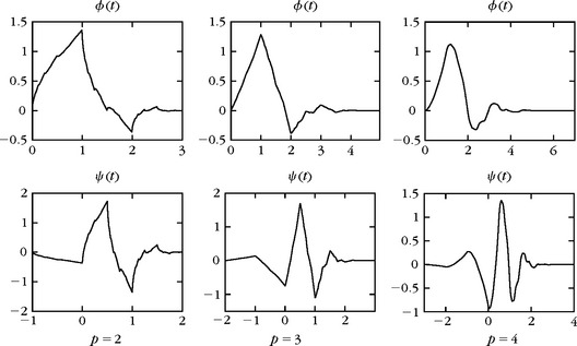
The regularity of ϕ and ψ is the same since ψ(t) is a finite linear combination of ϕ(2t – n). However, this regularity is difficult to estimate precisely. Let B = supω∈![]() |R(e −iω)| where R(e −iω) is the trigonometric polynomial defined in (7.91). Theorem 7.6 proves that ψ is at least uniformly Lipschitz α for α < p – log2 B − 1. For Daubechies wavelets, B increases more slowly than p, and Figure 7.10 shows indeed that the regularity of these wavelets increases with p. Daubechies and Lagarias [198] have established a more precise technique that computes the exact Lipschitz regularity of ψ. For p = 2 the wavelet ψ is only Lipschitz 0.55, but for p = 3 it is Lipschitz 1.08, which means that it is already continuously differentiable. For p large, ϕ and ψ are uniformly Lipschitz α, for α of the order of 0.2 p [168].
|R(e −iω)| where R(e −iω) is the trigonometric polynomial defined in (7.91). Theorem 7.6 proves that ψ is at least uniformly Lipschitz α for α < p – log2 B − 1. For Daubechies wavelets, B increases more slowly than p, and Figure 7.10 shows indeed that the regularity of these wavelets increases with p. Daubechies and Lagarias [198] have established a more precise technique that computes the exact Lipschitz regularity of ψ. For p = 2 the wavelet ψ is only Lipschitz 0.55, but for p = 3 it is Lipschitz 1.08, which means that it is already continuously differentiable. For p large, ϕ and ψ are uniformly Lipschitz α, for α of the order of 0.2 p [168].
Symmlets
Daubechies wavelets are very asymmetric because they are constructed by selecting the minimum-phase square root of Q(e −iω) in (7.97). One can show [51] that filters corresponding to a minimum-phase square root have their energy optimally concentrated near the starting point of their support. Thus, they are highly nonsymmetric, which yields very asymmetric wavelets.
To obtain a symmetric or antisymmetric wavelet, the filter h must be symmetric or antisymmetric with respect to the center of its support, which means that ĥ(ω) has a linear complex phase. Daubechies proved [194] that the Haar filter is the only real compactly supported conjugate mirror filter that has a linear phase. The Daubechies symmlet filters are obtained by optimizing the choice of the square root R(e −iω) of Q(e −iω) to obtain an almost linear phase. The resulting wavelets still have a minimum support [– p + 1, p] with p vanishing moments, but they are more symmetric, as illustrated by Figure 7.11 for p = 8. The coefficients of the symmlet filters are in WaveLab. Complex conjugate mirror filters with a compact support and a linear phase can be constructed [352], but they produce complex wavelet coefficients that have real and imaginary parts that are redundant when the signal is real.
Coiflets
For an application in numerical analysis, Coifman asked Daubechies [194] to construct a family of wavelets ψ that have p vanishing moments and a minimum-size support, with scaling functions that also satisfy
Such scaling functions are useful in establishing precise quadrature formulas. If f is Ck in the neighborhood of 2Jn with k < p, then a Taylor expansion of f up to order k shows that
Thus, at a fine scale 2J, the scaling coefficients are closely approximated by the signal samples. The order of approximation increases with p. The supplementary condition (7.99) requires increasing the support of ψ; the resulting coiflet has a support of size 3p − 1 instead of 2p − 1 for a Daubechies wavelet. The corresponding conjugate mirror filters are tabulated in WaveLab.
Audio Filters
The first conjugate mirror filters with finite impulse response were constructed in 1986 by Smith and Barnwell [443] in the context of perfect filter bank reconstruction, explained in Section 7.3.2. These filters satisfy the quadrature condition |ĥ(ω)|2 + |ĥ(ω + π)|2 = 2, which is necessary and sufficient for filter bank reconstruction. However, ĥ(0) ≠ √2, so the infinite product of such filters does not yield a wavelet basis of L2(![]() ). Instead of imposing any vanishing moments, Smith and Barnwell [443], and later Vaidyanathan and Hoang [470], designed their filters to reduce the size of the transition band, where |ĥ(ω)| decays from nearly √2 to nearly 0 in the neighborhood of ± π/2. This constraint is important in optimizing the transform code of audio signals (see Section 10.3.3). However, many cascades of these filters exhibit wild behavior. The Vaidyanathan-Hoang filters are tabulated in WaveLab. Many other classes of conjugate mirror filters with finite impulse response have been constructed [69, 79]. Recursive conjugate mirror filters may also be designed [300] to minimize the size of the transition band for a given number of zeroes at ω = π. These filters have a fast but noncausal recursive implementation for signals of finite size.
). Instead of imposing any vanishing moments, Smith and Barnwell [443], and later Vaidyanathan and Hoang [470], designed their filters to reduce the size of the transition band, where |ĥ(ω)| decays from nearly √2 to nearly 0 in the neighborhood of ± π/2. This constraint is important in optimizing the transform code of audio signals (see Section 10.3.3). However, many cascades of these filters exhibit wild behavior. The Vaidyanathan-Hoang filters are tabulated in WaveLab. Many other classes of conjugate mirror filters with finite impulse response have been constructed [69, 79]. Recursive conjugate mirror filters may also be designed [300] to minimize the size of the transition band for a given number of zeroes at ω = π. These filters have a fast but noncausal recursive implementation for signals of finite size.
7.3 WAVELETS AND FILTER BANKS
Decomposition coefficients in a wavelet orthogonal basis are computed with a fast algorithm that cascades discrete convolutions with h and g, and subsamples the output. Section 7.3.1 derives this result from the embedded structure of multiresolution approximations. A direct filter bank analysis is performed in Section 7.3.2, which gives more general perfect reconstruction conditions on the filters. Section 7.3.3 shows that perfect reconstruction filter banks decompose signals in a basis of ![]() 2(
2(![]() ). This basis is orthogonal for conjugate mirror filters.
). This basis is orthogonal for conjugate mirror filters.
7.3.1 Fast Orthogonal Wavelet Transform
We describe a fast filter bank algorithm that computes the orthogonal wavelet coefficients of a signal measured at a finite resolution. A fast wavelet transform decomposes successively each approximation ![]() into a coarser approximation
into a coarser approximation ![]() , plus the wavelet coefficients carried by
, plus the wavelet coefficients carried by ![]() . In the other direction, the reconstruction from wavelet coefficients recovers each
. In the other direction, the reconstruction from wavelet coefficients recovers each ![]() from
from ![]() and
and ![]() .
.
Since {ϕj, n}n∈![]() and {ψj, n}n∈
and {ψj, n}n∈![]() are orthonormal bases of Vj and Wj, the projection in these spaces is characterized by
are orthonormal bases of Vj and Wj, the projection in these spaces is characterized by
Theorem 7.10 [360, 361] shows that these coefficients are calculated with a cascade of discrete convolutions and subsamplings. We denote x[n] = x[–n] and
 (7.104)
Proof of (7.102).
Any ![]() can be decomposed in the orthonormal basis {ϕj, n}n∈
can be decomposed in the orthonormal basis {ϕj, n}n∈![]() of Vj:
of Vj:
With the change of variable t′ = 2−jt − 2p, we obtain
 (7.106)
Thus, (7.105) implies that
Computing the inner product of f with the vectors on each side of this equality yields (7.102).
Proof of (7.103).
Since ![]() , it can be decomposed as
, it can be decomposed as
As in (7.106), the change of variable t′ = 2−jt − 2p proves that
Taking the inner product with f on each side gives (7.103).
Proof of (7.104).
Since Wj+1 is the orthogonal complement of Vj+1 in Vj, the union of the two bases {ψj + 1, n}n∈![]() and {ϕj + 1, n}n∈
and {ϕj + 1, n}n∈![]() is an orthonormal basis of Vj. Thus, any ϕj, p can be decomposed in this basis:
is an orthonormal basis of Vj. Thus, any ϕj, p can be decomposed in this basis:

Inserting (7.106) and (7.108) yields
Taking the inner product with f on both sides of this equality gives (7.104).
Theorem 7.10 proves that aj+1 and dj+1 are computed by taking every other sample of the convolution of aj with ![]() and
and ![]() , respectively, as illustrated by Figure 7.12. The filter
, respectively, as illustrated by Figure 7.12. The filter ![]() removes the higher frequencies of the inner product sequence aj, whereas
removes the higher frequencies of the inner product sequence aj, whereas ![]() is a high-pass filter that collects the remaining highest frequencies. The reconstruction (7.104) is an interpolation that inserts zeroes to expand aj+1 and dj+1 and filters these signals, as shown in Figure 7.12.
is a high-pass filter that collects the remaining highest frequencies. The reconstruction (7.104) is an interpolation that inserts zeroes to expand aj+1 and dj+1 and filters these signals, as shown in Figure 7.12.
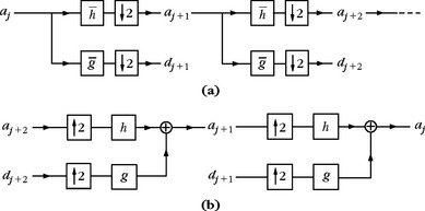
FIGURE 7.12 (a) A fast wavelet transform is computed with a cascade of filterings with ![]() and
and ![]() followed by a factor 2 subsampling. (b) A fast inverse wavelet transform reconstructs progressively each aj by inserting zeroes between samples of aj+1 and dj+1, filtering and adding the output.
followed by a factor 2 subsampling. (b) A fast inverse wavelet transform reconstructs progressively each aj by inserting zeroes between samples of aj+1 and dj+1, filtering and adding the output.
An orthogonal wavelet representation of aL = 〈f, ϕL, n〉 is composed of wavelet coefficients of f at scales 2L < 2j ≤ 2J, plus the remaining approximation at the largest scale 2J:
It is computed from aL by iterating (7.102) and (7.103) for L ≤ j < J. Figure 7.7 gives a numerical example computed with the cubic spline filter of Table 7.1. The original signal aL is recovered from this wavelet representation by iterating the reconstruction (7.104) for J > j ≥ L.
Initialization
Most often the discrete input signal b[n] is obtained by a finite-resolution device that averages and samples an analog input signal. For example, a CCD camera filters the light intensity by the optics and each photoreceptor averages the input light over its support. Thus, a pixel value measures average light intensity. If the sampling distance is N−1, to define and compute the wavelet coefficients, we need to associate to b[n] a function f(t) ∈ VL approximated at the scale 2L = N−1, and compute aL[n] = 〈f, ϕL, n〉. Exercise 7.6 explains how to compute aL[n] = 〈f, ϕL, n〉 so that b[n] = f(N−1n).
A simpler and faster approach considers
Since {ϕL, n(t) = 2−L/2 ϕ(2−Lt – n)}n∈![]() is orthonormal and 2L = N−1,
is orthonormal and 2L = N−1,
is a weighted average off in the neighborhood of N−1 n over a domain proportional to N−1. Thus, if f is regular,
If ψ is a coiflet and f(t) is regular in the neighborhood of N−1 n, then (7.100) shows that N−1/2 aL[n] is a high-order approximation of f(N−1 n).
Finite Signals
Let us consider a signal f with a support in [0, 1] and that is approximated with a uniform sampling at intervals N−1. The resulting approximation aL has N = 2−L samples. This is the case in Figure 7.7 with N = 1024. Computing the convolutions with ![]() and
and ![]() at abscissa close to 0 or close to N requires knowing the values of aL[n] beyond the boundaries n = 0 and n = N − 1. These boundary problems may be solved with one of the three approaches described in Section 7.5.
at abscissa close to 0 or close to N requires knowing the values of aL[n] beyond the boundaries n = 0 and n = N − 1. These boundary problems may be solved with one of the three approaches described in Section 7.5.
Section 7.5.1 explains the simplest algorithm, which periodizes aL. The convolutions in Theorem 7.10 are replaced by circular convolutions. This is equivalent to decomposing f in a periodic wavelet basis of L2[0, 1]. This algorithm has the disadvantage of creating large wavelet coefficients at the borders.
If ψ is symmetric or antisymmetric, we can use a folding procedure described in Section 7.5.2, which creates smaller wavelet coefficients at the border. It decomposes f in a folded wavelet basis of L2[0, 1]. However, we mentioned in Section 7.2.3 that Haar is the only symmetric wavelet with a compact support. Higher-order spline wavelets have a symmetry, but h must be truncated in numerical calculations.
The most efficient boundary treatment is described in Section 7.5.3, but the implementation is more complicated. Boundary wavelets that keep their vanishing moments are designed to avoid creating large-amplitude coefficients when f is regular. The fast algorithm is implemented with special boundary filters and requires the same number of calculations as the two other methods.
Complexity
Suppose that h and g have K nonzero coefficients. Let aL be a signal of size N = 2−L. With appropriate boundary calculations, each aj and dj has 2−j samples. Equations (7.102) and (7.103) compute aj+1 and dj+1 from aj with 2−jK additions and multiplications. Therefore, the wavelet representation (7.110) is calculated with at most 2KN additions and multiplications. The reconstruction (7.104) of aj from aj+1 and dj+1 is also obtained with 2−jK additions and multiplications. The original signal aL is also recovered from the wavelet representation with at most 2KN additions and multiplications.
Wavelet Graphs
The graphs of ϕ and ψ are computed numerically with the inverse wavelet transform. If f = ϕ, then a0[n] = δ[n] and dj[n] = 0 for all L < j ≤ 0. The inverse wavelet transform computes aL and (7.111) shows that
If ϕ is regular and N is large enough, we recover a precise approximation of the graph of ϕ from aL.
Similarly if f = ψ, then a0[n] = 0, d0[n] = δ[n], and dj[n] = 0 for L < j < 0. Then aL[n] is calculated with the inverse wavelet transform and N1/2 aL [n] ≈ ψ(N−1 n). The Daubechies wavelets and scaling functions in Figure 7.10 are calculated with this procedure.
7.3.2 Perfect Reconstruction Filter Banks
The fast discrete wavelet transform decomposes signals into low-pass and high-pass components subsampled by 2; the inverse transform performs the reconstruction. The study of such classical multirate filter banks became a major signal-processing topic in 1976, when Croisier, Esteban, and Galand [189] discovered that it is possible to perform such decompositions and reconstructions with quadrature mirror filters (Exercise 7.7). However, besides the simple Haar filter, a quadrature mirror filter cannot have a finite impulse response. In 1984, Smith and Barnwell [444] and Mintzer [376] found necessary and sufficient conditions for obtaining perfect reconstruction orthogonal filters with a finite impulse response that they called conjugate mirror filters. The theory was completed by the biorthogonal equations of Vetterli [471, 472] and the general paraunitary matrix theory of Vaidyanathan [469]. We follow this digital signal-processing approach, which gives a simple understanding of conjugate mirror filter conditions. More complete presentations of filter bank properties can be found in [1, 2, 63, 68, 69].
Filter Bank
A two-channel multirate filter bank convolves a signal a0 with a low-pass filter ![]() and a high-pass filter
and a high-pass filter ![]() and subsamples by 2 the output:
and subsamples by 2 the output:
A reconstructed signal ã0 is obtained by filtering the zero expanded signals with a dual low-pass filter ![]() and a dual high-pass filter
and a dual high-pass filter ![]() , as shown in Figure 7.13. With the zero insertion notation (7.101) it yields
, as shown in Figure 7.13. With the zero insertion notation (7.101) it yields
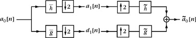
FIGURE 7.13 The input signal is filtered by a low-pass and a high-pass filter and subsampled. The reconstruction is performed by inserting zeroes and filtering with dual filters ![]() and
and ![]()
We study necessary and sufficient conditions on h, g, ![]() , and
, and ![]() to guarantee a perfect reconstruction ã0 = a0.
to guarantee a perfect reconstruction ã0 = a0.
Subsampling and Zero Interpolation
Subsamplings and expansions with zero insertions have simple expressions in the Fourier domain. Since ![]() , the Fourier series of the subsampled signal y[n] = x[2n] can be written as
, the Fourier series of the subsampled signal y[n] = x[2n] can be written as
The component ◯(ω + π) creates a frequency folding. This aliasing must be canceled at the reconstruction.
The insertion of zeros defines
Theorem 7.11 gives Vetterli’s [471] biorthogonal conditions, which guarantee that ã0 = a0.
Theorem 7.11:
Vetterli. The filter bank performs an exact reconstruction for any input signal if and only if
Proof.
We first relate the Fourier transform of a1 and d1 to the Fourier transform of a0. Since h and g are real, the transfer functions of ![]() and
and ![]() are, respectively,
are, respectively, ![]() and
and ![]() . By using (7.114), we derive from the definition (7.112) of a1 and d1 that
. By using (7.114), we derive from the definition (7.112) of a1 and d1 that
The expression (7.113) of ã0 and the zero insertion property (7.115) also imply
To obtain a0 = ã0 for all a0, the filters must cancel the aliasing term â0(ω + π) and guarantee a unit gain for â0(ω), which proves equations (7.116) and (7.117).
Theorem 7.11 proves that the reconstruction filters ![]() and
and ![]() are entirely specified by the decomposition filters h and g. In matrix form, it can be rewritten
are entirely specified by the decomposition filters h and g. In matrix form, it can be rewritten
 (7.121)
The inversion of this 2 × 2 matrix yields
 (7.122)
The reconstruction filters are stable only if the determinant does not vanish for all ω ∈ [–π, π]. Vaidyanathan [469] has extended this result to multirate filter banks with an arbitrary number M of channels by showing that the resulting matrices of filters satisfy paraunitary properties [68].
Finite Impulse Response
When all filters have a finite impulse response, the determinant Δ(ω) can be evaluated. This yields simpler relations between the decomposition and reconstruction filters.
Theorem 7.12.
Perfect reconstruction filters satisfy
For finite impulse-response filters, there exist a ∈ ![]() and l ∈
and l ∈ ![]() such that
such that
Proof.
Equation (7.122) proves that
The definition (7.123) implies that Δ(ω + π) = –Δ(ω). Inserting (7.127) in (7.117) yields (7.124).
The Fourier transform of finite impulse-response filters is a finite series in exp(± inω). Therefore, the determinant Δ(ω) defined by (7.123) is a finite series. Moreover, (7.126) proves that Δ−1 (ω) must also be a finite series. A finite series in exp(± inω) that has an inverse that is also a finite series must have a single term. Since Δ(ω) = –Δ(ω + π) the exponent n must be odd. This proves that there exist l ∈ ![]() and a ∈
and a ∈ ![]() such that
such that
Inserting this expression in (7.126) yields (7.125).
The factor a is a gain that is inverse for the decomposition and reconstruction filters and l is a reverse shift. We generally set a = 1 and l = 0. In the time domain (7.125) can then be rewritten as
The two pairs of filters (h, g) and (![]() ,
, ![]() ) play a symmetric role and can be inverted.
) play a symmetric role and can be inverted.
Conjugate Mirror Filters
If we impose that the decomposition filter h is equal to the reconstruction filter ![]() , then (7.124) is the condition of Smith and Barnwell [444] and Mintzer [376] that defines conjugate mirror filters:
, then (7.124) is the condition of Smith and Barnwell [444] and Mintzer [376] that defines conjugate mirror filters:
It is identical to the filter condition (7.29) that is required in order to synthesize orthogonal wavelets. Section 7.3.3 proves that it is also equivalent to discrete orthogonality properties.
7.3.3 Biorthogonal Bases of  2 (
2 ( )
)
The decomposition of a discrete signal in a multirate filter bank is interpreted as an expansion in a basis of ![]() 2 (
2 (![]() ). Observe first that the low-pass and high-pass signals of a filter bank computed with (7.112) can be rewritten as inner products in
). Observe first that the low-pass and high-pass signals of a filter bank computed with (7.112) can be rewritten as inner products in ![]() 2 (
2 (![]() ):
):
The signal recovered by the reconstructing filters is
 (7.133)
Inserting (7.131) and (7.132) yields
 (7.134)
We recognize the decomposition of a0 over dual families of vectors {![]() [n − 2l],
[n − 2l], ![]() [n − 2l]}l∈
[n − 2l]}l∈![]() and {h[n − 2l], g[n − 2l]}l∈
and {h[n − 2l], g[n − 2l]}l∈![]() . Theorem 7.13 proves that these two families are biorthogonal.
. Theorem 7.13 proves that these two families are biorthogonal.
Theorem 7.13.
If h, g, ![]() , and
, and ![]() are perfect reconstruction filters, and their Fourier transforms are bounded, then {
are perfect reconstruction filters, and their Fourier transforms are bounded, then {![]() [n − 2l],
[n − 2l], ![]() [n − 2l]}l∈
[n − 2l]}l∈![]() and {h[n − 2l], g[n − 2l]}l∈
and {h[n − 2l], g[n − 2l]}l∈![]() are biorthogonal Riesz bases of
are biorthogonal Riesz bases of ![]() 2(
2(![]() ).
).
Proof.
To prove that these families are biorthogonal we must show that for all n ∈ ![]()
For perfect reconstruction filters, (7.124) proves that
In the time domain, this equation becomes
 (7.138)
which verifies (7.135). The same proof as for (7.124) shows that
In the time domain, this equation yields (7.136). It also follows from (7.122) that
The inverse Fourier transforms of these two equations yield (7.137).
To finish the proof, one must show the existence of Riesz bounds. The reader can verify that this is a consequence of the fact that the Fourier transform of each filter is bounded.
Orthogonal Bases
A Riesz basis is orthonormal if the dual basis is the same as the original basis. For filter banks this means that h = ![]() and g =
and g = ![]() . The filter h is then a conjugate mirror filter
. The filter h is then a conjugate mirror filter
The resulting family {h[n − 2l], g[n − 2l]}l∈![]() is an orthogonal basis of
is an orthogonal basis of ![]() 2(
2(![]() ).
).
Discrete Wavelet Bases
The construction of conjugate mirror filters is simpler than the construction of orthogonal wavelet bases of L2(![]() ). Why then should we bother with continuous time models of wavelets, since in any case, all computations are discrete and rely on conjugate mirror filters? The reason is that conjugate mirror filters are most often used in filter banks that cascade several levels of filterings and subsamplings. Thus, it is necessary to understand the behavior of such a cascade [407]. In a wavelet filter bank tree, the output of the low-pass filter
). Why then should we bother with continuous time models of wavelets, since in any case, all computations are discrete and rely on conjugate mirror filters? The reason is that conjugate mirror filters are most often used in filter banks that cascade several levels of filterings and subsamplings. Thus, it is necessary to understand the behavior of such a cascade [407]. In a wavelet filter bank tree, the output of the low-pass filter ![]() is subdecomposed, whereas the output of the high-pass filter
is subdecomposed, whereas the output of the high-pass filter ![]() is not; this is illustrated in Figure 7.12. Suppose that the sampling distance of the original discrete signal is N−1. We denote aL[n] for this discrete signal, with 2L = N−1. At the depth j – L ≥ 0 of this filter bank tree, the low-pass signal aj and high-pass signal dj can be written as
is not; this is illustrated in Figure 7.12. Suppose that the sampling distance of the original discrete signal is N−1. We denote aL[n] for this discrete signal, with 2L = N−1. At the depth j – L ≥ 0 of this filter bank tree, the low-pass signal aj and high-pass signal dj can be written as
The Fourier transforms of these equivalent filters are
 (7.140)
A filter bank tree of depth J – L ≥ 0 decomposes aL over the family of vectors
For conjugate mirror filters, one can verify that this family is an orthonormal basis of ![]() 2 (
2 (![]() ). These discrete vectors are close to a uniform sampling of the continuous time-scaling functions ϕj(t) = 2−j/2 ϕ(2−jt) and wavelets ψj(t) = 2−j/2 ϕ(2−j t). When the number L – j of successive convolutions increases, one can verify that ϕj[n] and ψj[n] converge, respectively, to N−1/2 ϕj(N−1n) and N−1/2 ψj(N−1n).
). These discrete vectors are close to a uniform sampling of the continuous time-scaling functions ϕj(t) = 2−j/2 ϕ(2−jt) and wavelets ψj(t) = 2−j/2 ϕ(2−j t). When the number L – j of successive convolutions increases, one can verify that ϕj[n] and ψj[n] converge, respectively, to N−1/2 ϕj(N−1n) and N−1/2 ψj(N−1n).
The factor N−1/2 normalizes the ![]() 2 (
2 (![]() ) norm of these sampled functions. If L – j = 4, then ϕj[n] and ψj[n] are already very close to these limit values. Thus, the impulse responses ϕj[n] and ψj[n] of the filter bank are much closer to continuous time-scaling functions and wavelets than they are to the original conjugate mirror filters h and g. This explains why wavelets provide appropriate models for understanding the applications of these filter banks. Chapter 8 relates more general filter banks to wavelet packet bases.
) norm of these sampled functions. If L – j = 4, then ϕj[n] and ψj[n] are already very close to these limit values. Thus, the impulse responses ϕj[n] and ψj[n] of the filter bank are much closer to continuous time-scaling functions and wavelets than they are to the original conjugate mirror filters h and g. This explains why wavelets provide appropriate models for understanding the applications of these filter banks. Chapter 8 relates more general filter banks to wavelet packet bases.
If the decomposition and reconstruction filters of the filter bank are different, the resulting basis (7.141) is nonorthogonal. The stability of this discrete wavelet basis does not degrade when the depth J – L of the filter bank increases. The next section shows that the corresponding continuous time wavelet ψ(t) generates a Riesz basis of L2(R).