The Basis of Recurrence

To understand how recurrence might work, let’s first consider the limitations of the models used thus far in the book. Ultimately, creating a model looks a little bit like Figure 7-1. You provide data and labels and define a model architecture, and the model learns the rules that fit the data to the labels. Those rules then become available to you as an API that will give you back predicted labels for future data.

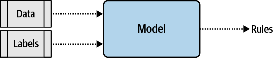
Figure 7-1. High-level view of model creation

But as you can see, the data is lumped in wholesale. There’s no granularity involved, and no effort to understand the sequence in which that data occurs. This means the words “blue” and “sky” have no different meaning in sentences such as “today I am blue, because the sky is gray” and “today I am happy, and there’s a beautiful blue sky”. To us the difference in the use of these words is obvious, but to a model with the architecture shown here there really is no difference.

So how do we fix this? Let’s first explore the nature of recurrence, and from there you’ll be able to see how a basic RNN can work.

Consider the famous Fibonacci sequence of numbers. In case you aren’t familiar with it, I’ve put some of them into Figure 7-2.

Figure 7-2. The first few numbers in the Fibonacci sequence

The idea behind this sequence is that every number is the sum of the two numbers preceding it. So if we start with 1 and 2, the next number is 1+2, which is 3. The one after that is 2+3, which is 5, then 3+5, which is 8, and so on.

We can place this in a computational graph to get Figure 7-3.

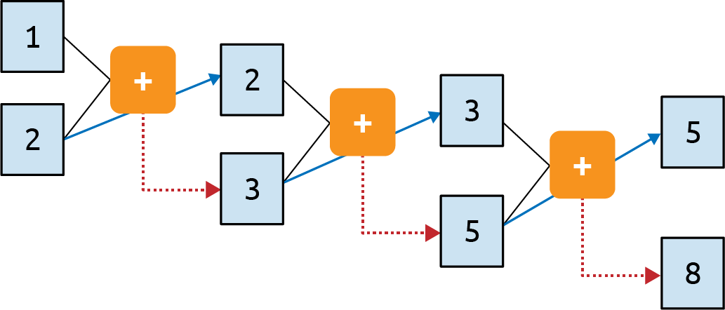
Figure 7-3. A computational graph representation of the Fibonacci sequence

Here you can see that we feed 1 and 2 into the function and get 3 as the output. We carry the second parameter (2) over to the next step, and feed it into the function along with the output from the previous step (3). The output of this is 5, and it gets fed into the function with the second parameter from the previous step (3) to produce an output of 8. This process continues indefinitely, with every operation depending on those before it. The 1 at the top left sort of “survives” through the process. It’s an element of the 3 that gets fed into the second operation, it’s an element of the 5 that gets fed into the third, and so on. Thus, some of the essence of the 1 is preserved throughout the sequence, though its impact on the overall value is diminished.

This is analogous to how a recurrent neuron is architected. You can see the typical representation of a recurrent neuron in Figure 7-4.

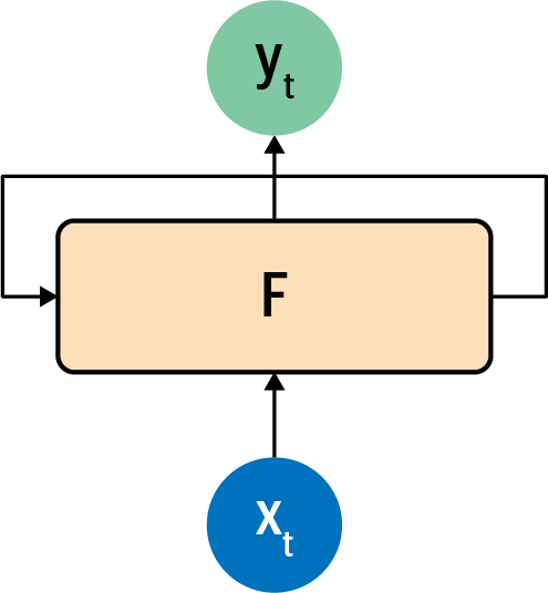
Figure 7-4. A recurrent neuron

A value x is fed into the function F at a time step, so it’s typically labeled x_t. This produces an output y at that time step, which is typically labeled y_t. It also produces a value that is fed forward to the next step, which is indicated by the arrow from F to itself.

This is made a little clearer if you look at how recurrent neurons work beside each other across time steps, which you can see in Figure 7-5.

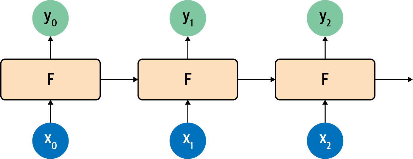
Figure 7-5. Recurrent neurons in time steps

Here, x₀ is operated on to get y₀ and a value that’s passed forward. The next step gets that value and x₁ and produces y₁ and a value that’s passed forward. The next one gets that value and x₂ and produces y₂ and a pass-forward value, and so on down the line. This is similar to what we saw with the Fibonacci sequence, and I always find that to be a handy mnemonic when trying to remember how an RNN works!

Extending Recurrence for Language

In the previous section you saw how a recurrent neural network operating over several time steps can help maintain context across a sequence. Indeed, RNNs will be used for sequence modeling later in this book. But there’s a nuance when it comes to language that can be missed when using a simple RNN like those in Figure 7-4 and Figure 7-5. As in the Fibonacci sequence example mentioned earlier, the amount of context that’s carried over will diminish over time. The effect of the output of the neuron at step 1 is huge at step 2, smaller at step 3, smaller still at step 4, and so on. So if we have a sentence like “Today has a beautiful blue <something>”, the word “blue” will have a strong impact on the next word; we can guess that it’s likely to be “sky”. But what about context that comes from further back in a sentence? For example, consider the sentence “I lived in Ireland, so in high school I had to learn how to speak and write <something>”.

That <something> is Gaelic, but the word that really gives us that context is “Ireland”, which is much further back in the sentence. Thus, for us to be able to recognize what <something> should be, a way for context to be preserved across a longer distance is needed. The short-term memory of an RNN needs to get longer, and in recognition of this an enhancement to the architecture, called long short-term memory (LSTM), was invented.

While I won’t go into detail on the underlying architecture of how LSTMs work, the high-level diagram shown in Figure 7-6 gets the main point across. To learn more about the internal operations, check out Christopher Olah’s excellent blog post on the subject.

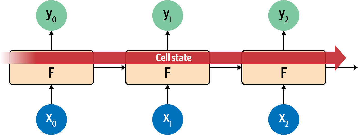
Figure 7-6. High-level view of LSTM architecture

The LSTM architecture enhances the basic RNN by adding a “cell state” that enables context to be maintained not just from step to step, but across the entire sequence of steps. Remembering that these are neurons, learning in the way neurons do, you can see that this ensures that the context that is important will be learned over time.

An important part of an LSTM is that it can be bidirectional—the time steps are iterated both forwards and backwards, so that context can be learned in both directions. See Figure 7-7 for a high-level view of this.

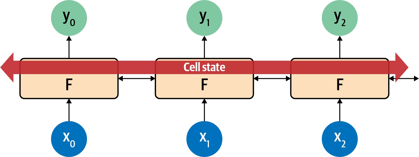
Figure 7-7. High-level view of LSTM bidirectional architecture

In this way evaluation in the direction from 0 to number_of_steps is done, as is evaluation from number_of_steps to 0. At each step, the y result is an aggregation of the “forward” pass and the “backward” pass. You can see this in Figure 7-8.

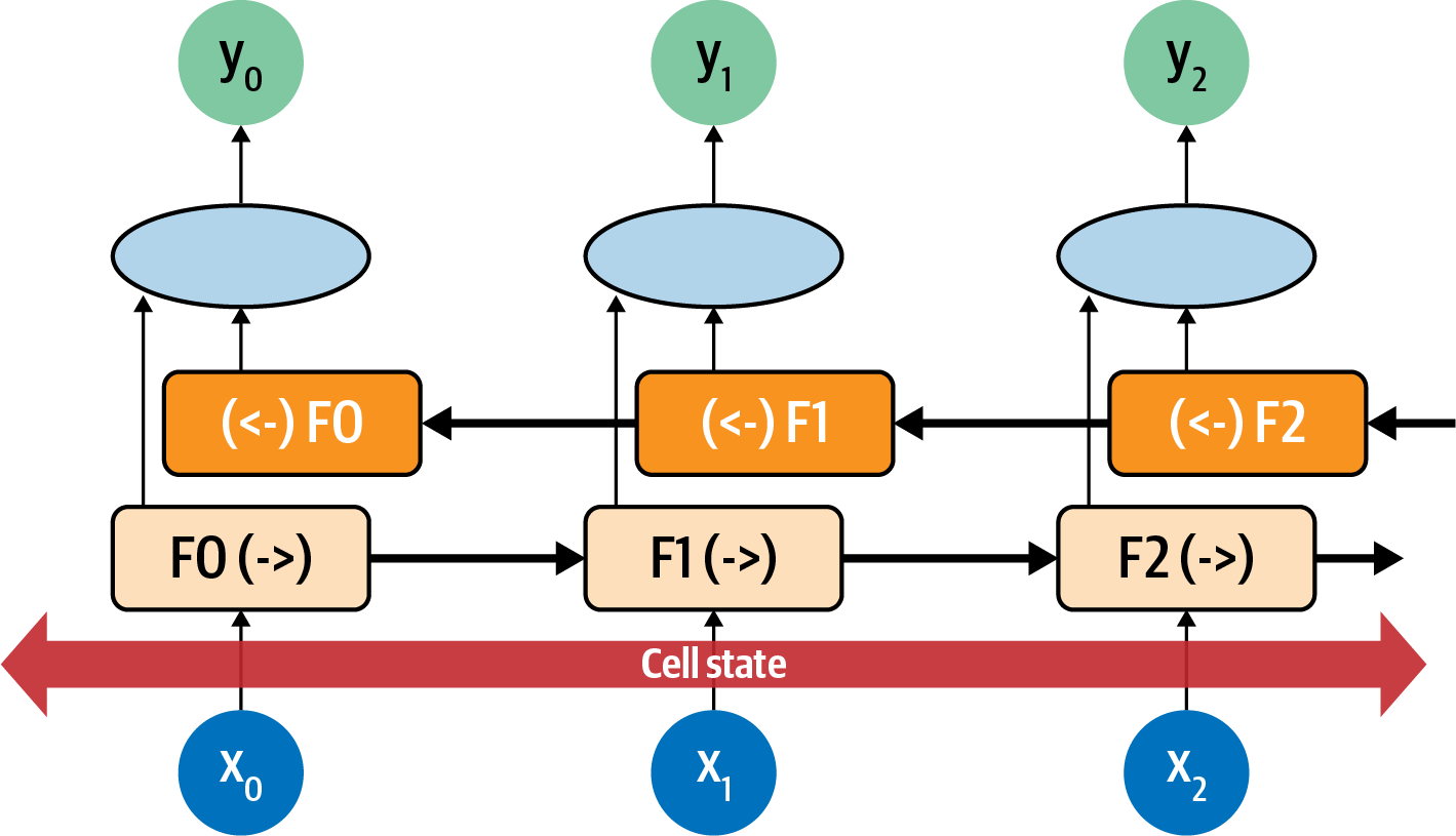
Figure 7-8. Bidirectional LSTM

In this case, consider each neuron at each time step to be F0, F1, F2, etc. The direction of the time step is shown, so the calculation at F1 in the forward direction is F1(->), and in the reverse direction it’s (<-)F1. The values of these are aggregated to give the y value for that time step. Additionally, the cell state is bidirectional. This can be really useful for managing context in sentences. Again considering the sentence “I lived in Ireland, so in high school I had to learn how to speak and write <something>”, you can see how the <something> was qualified to be “Gaelic” by the context word “Ireland”. But what if it were the other way around: “I lived in <this country>, so in high school I had to learn how to speak and write Gaelic”? You can see that by going backwards through the sentence we can learn about what <this country> should be. Thus, using bidirectional LSTMs can be very powerful for understanding sentiment in text (and as you’ll see in Chapter 8, they’re really powerful for generating text too!).

Of course, there’s a lot going on with LSTMs, in particular bidirectional ones, so expect training to be slow. Here’s where it’s worth investing in a GPU, or at the very least using a hosted one in Google Colab if you can.

Creating a Text Classifier with RNNs

In Chapter 6 you experimented with creating a classifier for the Sarcasm dataset using embeddings. In that case words were turned into vectors before being aggregated and then fed into dense layers for classification. When using an RNN layer such as an LSTM, you don’t do the aggregation and can feed the output of the embedding layer directly into the recurrent layer. When it comes to the dimensionality of the recurrent layer, a rule of thumb you’ll often see is that it’s the same size as the embedding dimension. This isn’t necessary, but can be a good starting point. Note that while in Chapter 6 I mentioned that the embedding dimension is often the fourth root of the size of the vocabulary, when using RNNs you’ll often see that that rule is ignored because it would make the size of the recurrent layer too small.

So, for example, the simple model architecture for the sarcasm classifier you developed in Chapter 6 could be updated to this to use a bidirectional LSTM:

	model = tf.keras.Sequential([
    tf.keras.layers.Embedding(vocab_size, embedding_dim),
    tf.keras.layers.Bidirectional(tf.keras.layers.LSTM(embedding_dim)),
    tf.keras.layers.Dense(24, activation='relu'),
    tf.keras.layers.Dense(1, activation='sigmoid')
])

The loss function and classifier can be set to this (note that the learning rate is .00001, or 1e-5):

	adam = tf.keras.optimizers.Adam(learning_rate=0.00001, 
                                beta_1=0.9, beta_2=0.999, amsgrad=False)

model.compile(loss='binary_crossentropy',
              optimizer=adam, metrics=['accuracy'])

When you print out the model architecture summary, you’ll see something like this. Note that the vocab size is 20,000 and the embedding dimension is 64. This gives 1,280,000 parameters in the embedding layer, and the bidirectional layer will have 128 neurons (64 out, 64 back) :

	Layer (type)                 Output Shape              Param #   
=================================================================
embedding_11 (Embedding)     (None, None, 64)          1280000   
_________________________________________________________________
bidirectional_7 (Bidirection (None, 128)               66048     
_________________________________________________________________
dense_18 (Dense)             (None, 24)                3096      
_________________________________________________________________
dense_19 (Dense)             (None, 1)                 25        
=================================================================
Total params: 1,349,169
Trainable params: 1,349,169
Non-trainable params: 0
_________________________________________________________________

Figure 7-9 shows the results of training with this over 30 epochs.

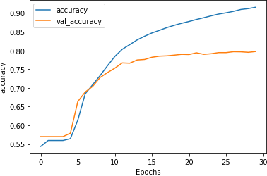
Figure 7-9. Accuracy for LSTM over 30 epochs

As you can see, the accuracy of the network on training data rapidly climbs above 90%, but the validation data plateaus at around 80%. This is similar to the figures we got earlier, but inspecting the loss chart in Figure 7-10 shows that while the loss for the validation set diverged after 15 epochs, it also flattened out to a much lower value than the loss charts in Chapter 6, despite using 20,000 words instead of 2,000.

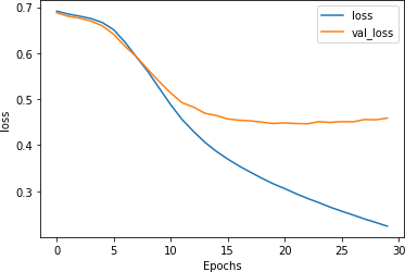
Figure 7-10. Loss with LSTM over 30 epochs

This was just using a single LSTM layer, however. In the next section you’ll see how to use stacked LSTMs and explore the impact on the accuracy of classifying this dataset.

Stacking LSTMs

In the previous section you saw how to use an LSTM layer after the embedding layer to help with classifying the contents of the Sarcasm dataset. But LSTMs can be stacked on top of each other, and this approach is used in many state-of-the-art NLP models.

Stacking LSTMs with TensorFlow is pretty straightforward. You add them as extra layers just like you would with a Dense layer, but with the exception that all of the layers prior to the last one will need to have their return_sequences property set to True. Here’s an example:

	model = tf.keras.Sequential([
    tf.keras.layers.Embedding(vocab_size, embedding_dim),
    tf.keras.layers.Bidirectional(tf.keras.layers.LSTM(embedding_dim, 
return_sequences=True)),
    tf.keras.layers.Bidirectional(tf.keras.layers.LSTM(embedding_dim)),
    tf.keras.layers.Dense(24, activation='relu'),
    tf.keras.layers.Dense(1, activation='sigmoid')
])

The final layer can also have return_sequences=True set, in which case it will return sequences of values to the dense layers for classification instead of single ones. This can be handy when parsing the output of the model, as we’ll discuss later.

The model architecture will look like this:

	Layer (type)                 Output Shape              Param #   
=================================================================
embedding_12 (Embedding)     (None, None, 64)          1280000   
_________________________________________________________________
bidirectional_8 (Bidirection (None, None, 128)         66048     
_________________________________________________________________
bidirectional_9 (Bidirection (None, 128)               98816     
_________________________________________________________________
dense_20 (Dense)             (None, 24)                3096      
_________________________________________________________________
dense_21 (Dense)             (None, 1)                 25        
=================================================================
Total params: 1,447,985
Trainable params: 1,447,985
Non-trainable params: 0
_________________________________________________________________

Adding the extra layer will give us roughly 100,000 extra parameters that need to be learned, an increase of about 8%. So, it might slow the network down, but the cost is relatively low if there’s a reasonable benefit.

After training for 30 epochs, the result looks like Figure 7-11. While the accuracy on the validation set is flat, examining the loss (Figure 7-12) tells a different story.

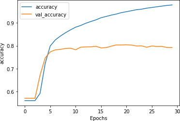
Figure 7-11. Accuracy for stacked LSTM architecture

As you can see in Figure 7-12, while the accuracy for both training and validation looked good, the validation loss quickly took off upwards, a clear sign of overfitting.

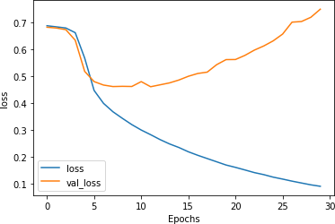
Figure 7-12. Loss for stacked LSTM architecture

This overfitting—indicated by the training accuracy climbing toward 100% as the loss falls smoothly, while the validation accuracy is relatively steady and the loss increases drastically—is a result of the model getting overspecialized for the training set. As with the examples in Chapter 6, this shows that it’s easy to be lulled into a false sense of security if you just look at the accuracy metrics without examining the loss.

Optimizing stacked LSTMs

In Chapter 6 you saw that a very effective method to reduce overfitting was to reduce the learning rate. It’s worth exploring whether that will have a positive effect on a recurrent neural network too.

For example, the following code reduces the learning rate by 20% from .00001 to .000008:

	adam = tf.keras.optimizers.Adam(learning_rate=0.000008, 
  beta_1=0.9, beta_2=0.999, amsgrad=False)

model.compile(loss='binary_crossentropy',
  optimizer=adam,metrics=['accuracy'])

Figure 7-13 demonstrates the impact of this on training. There doesn’t seem to be much of a difference, although the curves (particularly for the validation set) are a little smoother.

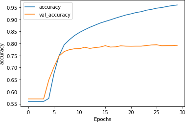
Figure 7-13. Impact of reduced learning rate on accuracy with stacked LSTMs

While an initial look at Figure 7-14 similarly suggests minimal impact on loss due to the reduced learning rate, it’s worth looking a little closer. Despite the shape of the curve being roughly similar, the rate of loss increase is clearly lower: after 30 epochs it’s at around 0.6, whereas with the higher learning rate it was close to 0.8. Adjusting the learning rate hyperparameter certainly seems worth investigation!

Figure 7-14. Impact of reduced learning rate on loss with stacked LSTMs

Using dropout

In addition to changing the learning rate parameter, it’s also worth considering using dropout in the LSTM layers. It works exactly the same as for dense layers, as discussed in Chapter 3, where random neurons are dropped to prevent a proximity bias from impacting the learning.

Dropout can be implemented using a parameter on the LSTM layer. Here’s an example:

	model = tf.keras.Sequential([
    tf.keras.layers.Embedding(vocab_size, embedding_dim),
    tf.keras.layers.Bidirectional(tf.keras.layers.LSTM(embedding_dim,
return_sequences=True, dropout=0.2)),
    tf.keras.layers.Bidirectional(tf.keras.layers.LSTM(embedding_dim,
dropout=0.2)),
    tf.keras.layers.Dense(24, activation='relu'),
    tf.keras.layers.Dense(1, activation='sigmoid')
])

Do note that implementing dropout will greatly slow down your training. In my case, using Colab, it went from ~10 seconds per epoch to ~180 seconds.

The accuracy results can be seen in Figure 7-15.

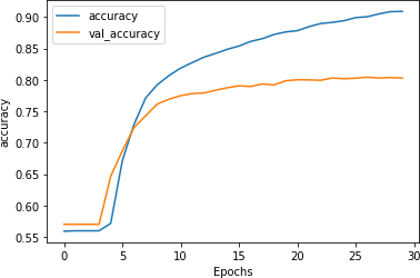
Figure 7-15. Accuracy of stacked LSTMs using dropout

As you can see using dropout doesn’t have much impact on the accuracy of the network, which is good! There’s always a worry that losing neurons will make your model perform worse, but as we can see here that’s not the case.

There’s also a positive impact on loss, as you can see in Figure 7-16.

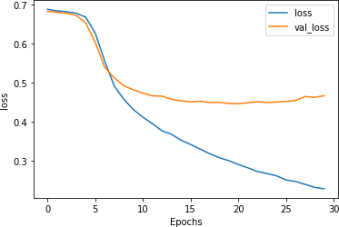
Figure 7-16. Loss curves for dropout-enabled LSTMs

While the curves are clearly diverging, they are closer than they were previously, and the validation set is flattening out at a loss of about 0.5. That’s significantly better than the 0.8 seen previously! As this example shows, dropout is another handy technique that you can use to improve the performance of LSTM-based RNNs.

It’s worth exploring these techniques to avoid overfitting in your data, as well as the techniques to preprocess your data that we covered in Chapter 6. But there’s one thing that we haven’t yet tried—a form of transfer learning where you can use prelearned embeddings for words instead of trying to learn your own. We’ll explore that next.

Using Pretrained Embeddings with RNNs

In all the previous examples you gathered the full set of words to be used in the training set, then trained embeddings with them. These were initially aggregated before being fed into a dense network, and in this chapter you explored how to improve the results using an RNN. While doing this, you were restricted to the words in your dataset and how their embeddings could be learned using the labels from that dataset.

Think back to Chapter 4, where we discussed transfer learning. What if, instead of learning the embeddings for yourself, you could instead use prelearned embeddings, where researchers have already done the hard work of turning words into vectors and those vectors are proven? One example of this is the GloVe (Global Vectors for Word Representation) model developed by Jeffrey Pennington, Richard Socher, and Christopher Manning at Stanford.

In this case, the researchers have shared their pretrained word vectors for a variety of datasets:

• A 6-billion-token, 400-thousand-word vocab set in 50, 100, 200, and 300 dimensions with words taken from Wikipedia and Gigaword

• A 42-billion-token, 1.9-million-word vocab in 300 dimensions from a common crawl

• An 840-billion-token, 2.2-million-word vocab in 300 dimensions from a common crawl

• A 27-billion-token, 1.2-million-word vocab in 25, 50, 100 and 200 dimensions from a Twitter crawl of 2 billion tweets

Given that the vectors are already pretrained, it’s simple to reuse them in your TensorFlow code, instead of learning from scratch. First, you’ll have to download the GloVe data. I’ve opted to use the Twitter data with 27 billion tokens and a 1.2-million-word vocab. The download is an archive with 25, 50, 100, and 200 dimensions.

To make it a little easier for you I’ve hosted the 25-dimension version, and you can download it into a Colab notebook like this:

	!wget --no-check-certificate 
    https://storage.googleapis.com/laurencemoroney-blog.appspot.com
           /glove.twitter.27B.25d.zip 
    -O /tmp/glove.zip

It’s a ZIP file, so you can extract it like this to get a file called glove.twitter.27b.25d.txt:

	# Unzip GloVe embeddings
import os
import zipfile

local_zip = '/tmp/glove.zip'
zip_ref = zipfile.ZipFile(local_zip, 'r')
zip_ref.extractall('/tmp/glove')
zip_ref.close()

Each entry in the file is a word, followed by the dimensional coefficients that were learned for it. The easiest way to use this is to create a dictionary where the key is the word, and the values are the embeddings. You can set up this dictionary like this:

	glove_embeddings = dict()
f = open('/tmp/glove/glove.twitter.27B.25d.txt')
for line in f:
    values = line.split()
    word = values[0]
    coefs = np.asarray(values[1:], dtype='float32')
    glove_embeddings[word] = coefs
f.close()

At this point you’ll be able to look up the set of coefficients for any word simply by using it as the key. So, for example, to see the embeddings for “frog”, you could use:

	glove_embeddings['frog']

With this resource in hand, you can use the tokenizer to get the word index for your corpus as before—but now you can create a new matrix, which I’ll call the embedding matrix. This will use the embeddings from the GloVe set (taken from glove_embeddings) as its values. So, if you examine the words in the word index for your dataset, like this:

	{'<OOV>': 1, 'new': 2, … 'not': 5, 'just': 6, 'will': 7

Then the first row in the embedding matrix should be the coefficients from GloVe for “<OOV>”, the next row will be the coefficients for “new”, and so on.

You can create that matrix with this code:

	embedding_matrix = np.zeros((vocab_size, embedding_dim))
for word, index in tokenizer.word_index.items():
    if index > vocab_size - 1:
        break
    else:
        embedding_vector = glove_embeddings.get(word)
        if embedding_vector is not None:
            embedding_matrix[index] = embedding_vector

This simply creates a matrix with the dimensions of your desired vocab size and the embedding dimension. Then, for every item in the tokenizer’s word index, you look up the coefficients from GloVe in glove_embeddings, and add those values to the matrix.

You then amend the embedding layer to use the pretrained embeddings by setting the weights parameter, and specify that you don’t want the layer to be trained by setting trainable=False:

	model = tf.keras.Sequential([
    tf.keras.layers.Embedding(vocab_size, embedding_dim, 
                              weights=[embedding_matrix], trainable=False),
    tf.keras.layers.Bidirectional(tf.keras.layers.LSTM(embedding_dim, 
                                  return_sequences=True)),
    tf.keras.layers.Bidirectional(tf.keras.layers.LSTM(embedding_dim)),
    tf.keras.layers.Dense(24, activation='relu'),
    tf.keras.layers.Dense(1, activation='sigmoid')
])

You can now train as before. However, you’ll want to consider your vocab size. One of the optimizations you did in the previous chapter to avoid overfitting was intended to prevent the embeddings becoming overburdened with learning low-frequency words; you avoided overfitting by using a smaller vocabulary of frequently used words. In this case, as the word embeddings have already been learned for you with GloVe, you could expand the vocabulary—but by how much?

The first thing to explore is how many of the words in your corpus are actually in the GloVe set. It has 1.2 million words, but there’s no guarantee it has all of your words.

So, here’s some code to perform a quick comparison so you can explore how large your vocab should be.

First let’s sort the data out. Create a list of Xs and Ys, where X is the word index, and Y=1 if the word is in the embeddings and 0 if it isn’t. Additionally, you can create a cumulative set, where you count the quotient of words at every time step. For example, the word “OOV” at index 0 isn’t in GloVe, so its cumulative Y would be 0. The word “new”, at the next index, is in GloVe, so it’s cumulative Y would be 0.5 (i.e., half of the words seen so far are in GloVe), and you’d continue to count that way for the entire dataset:

	xs=[]
ys=[]
cumulative_x=[]
cumulative_y=[]
total_y=0
for word, index in tokenizer.word_index.items():
  xs.append(index)
  cumulative_x.append(index)
  if glove_embeddings.get(word) is not None:
    total_y = total_y + 1
    ys.append(1)
  else:
    ys.append(0)
  cumulative_y.append(total_y / index)

You then plot the Xs against the Ys with this code:

	import matplotlib.pyplot as plt
fig, ax = plt.subplots(figsize=(12,2))
ax.spines['top'].set_visible(False)

plt.margins(x=0, y=None, tight=True)
#plt.axis([13000, 14000, 0, 1])
plt.fill(ys)

This will give you a word frequency chart, which will look something like Figure 7-17.

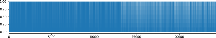
Figure 7-17. Word frequency chart

As you can see in the chart, the density changes somewhere between 10,000 and 15,000. This gives you an eyeball check that somewhere around token 13,000 the frequency of words that are not in the GloVe embeddings starts to outpace those that are.

If you then plot the cumulative_x against the cumulative_y, you can get a better sense of this. Here’s the code:

	import matplotlib.pyplot as plt
plt.plot(cumulative_x, cumulative_y)
plt.axis([0, 25000, .915, .985])

You can see the results in Figure 7-18.

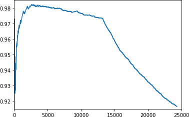
Figure 7-18. Plotting frequency of word index against GloVe

You can now tweak the parameters in plt.axis to zoom in to find the inflection point where words not present in GloVe begin to outpace those that are in GloVe. This is a good starting point for you to set the size of your vocabulary.

Using this method I chose to use a vocab size of 13,200 (instead of the 2,000 that was previously used to avoid overfitting) and this model architecture, where the embedding_dim is 25 because of the GloVe set I’m using.:

	model = tf.keras.Sequential([
    tf.keras.layers.Embedding(vocab_size, embedding_dim, 
weights=[embedding_matrix], trainable=False),
    tf.keras.layers.Bidirectional(tf.keras.layers.LSTM(embedding_dim, 
return_sequences=True)),
    tf.keras.layers.Bidirectional(tf.keras.layers.LSTM(embedding_dim)),
    tf.keras.layers.Dense(24, activation='relu'),
    tf.keras.layers.Dense(1, activation='sigmoid')
])
adam = tf.keras.optimizers.Adam(learning_rate=0.00001, beta_1=0.9, beta_2=0.999,
amsgrad=False)
model.compile(loss='binary_crossentropy',optimizer=adam, metrics=['accuracy'])

Training this for 30 epochs yields some excellent results. The accuracy is shown in Figure 7-19. The validation accuracy is very close to the training accuracy, indicating that we are no longer overfitting.

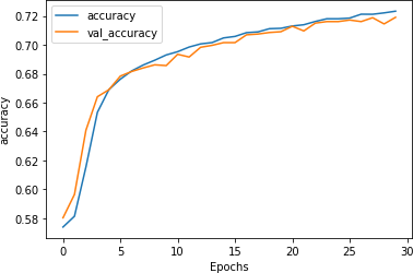
Figure 7-19. Stacked LSTM accuracy using GloVe embeddings

This is reinforced by the loss curves, as shown in Figure 7-20. The validation loss no longer diverges, showing that although our accuracy is only ~73% we can be confident that the model is accurate to that degree.

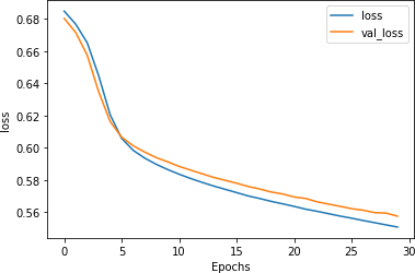
Figure 7-20. Stacked LSTM loss using GloVe embeddings

Training the model for longer shows very similar results, and indicates that while overfitting begins to occur right around epoch 80, the model is still very stable.

The accuracy metrics (Figure 7-21) show a well-trained model.

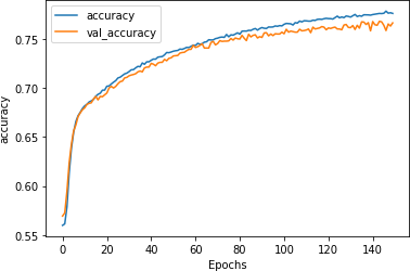
Figure 7-21. Accuracy on stacked LSTM with GloVe over 150 epochs

The loss metrics (Figure 7-22) show the beginning of divergence at around epoch 80, but the model still fits well.

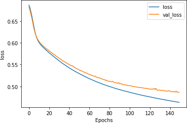
Figure 7-22. Loss on stacked LSTM with GloVe over 150 epochs

This tells us that this model is a good candidate for early stopping, where you can just train it for 75–80 epochs to get the optimal results.

I tested it with headlines from The Onion, source of the sarcastic headlines in the Sarcasm dataset, against other sentences, as shown here:

	test_sentences = ["It Was, For, Uh, Medical Reasons, Says Doctor To Boris Johnson,
Explaining Why They Had To Give Him Haircut",

"It's a beautiful sunny day",

"I lived in Ireland, so in high school they made me learn to speak and write in
Gaelic",

"Census Foot Soldiers Swarm Neighborhoods, Kick Down Doors To Tally Household
Sizes"]

The results for these headlines are as follows—remember that values close to 50% (0.5) are considered neutral, close to 0 non-sarcastic, and close to 1 sarcastic:

	[[0.8170955 ]
 [0.08711044]
 [0.61809343]
 [0.8015281 ]]

The first and fourth sentences, taken from The Onion, showed 80%+ likelihood of sarcasm. The statement about the weather was strongly non-sarcastic (9%), and the sentence about going to high school in Ireland was deemed to be potentially sarcastic, but not with high confidence (62%).

Summary

This chapter introduced you to recurrent neural networks, which use sequence-oriented logic in their design and can help you understand the sentiment in sentences based not only on the words they contain, but also the order in which they appear. You saw how a basic RNN works, as well as how an LSTM can build on this to enable context to be preserved over the long term. You used these to improve the sentiment analysis model you’ve been working on. You then looked into overfitting issues with RNNs and techniques to improve them, including using transfer learning from pretrained embeddings. In Chapter 8 you’ll use what you’ve learned to explore how to predict words, and from there you’ll be able to create a model that creates text, writing poetry for you!