What Is TensorFlow Serving?

This book has primarily focused on the code for creating models, and while this is a massive undertaking in itself, it’s only a small part of the overall picture of what it takes to use machine learning models in production. As you can see in Figure 19-1, your code needs to work alongside code for configuration, data collection, data verification, monitoring, machine resource management, and feature extraction, as well as analysis tools, process management tools, and serving infrastructure.

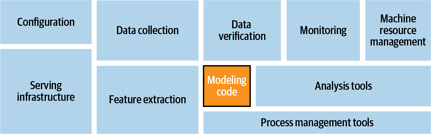
Figure 19-1. System architecture modules for ML systems

TensorFlow’s ecosystem for these tools is called TensorFlow Extended (TFX). Other than the serving infrastructure, covered in this chapter, I won’t be going into any of the rest of TFX. A great resource if you’d like to learn more about it is the book Building Machine Learning Pipelines: Automating Model Life Cycles with TensorFlow by Hannes Hapke and Catherine Nelson (O’Reilly).

The pipeline for machine learning models is summarized in Figure 19-2.

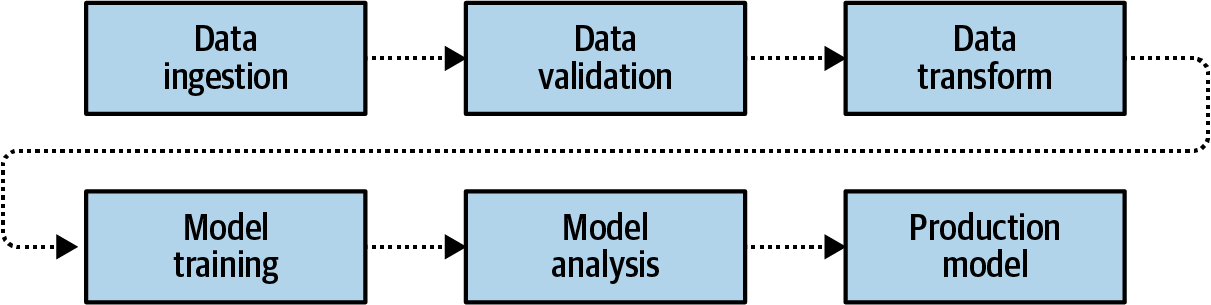
Figure 19-2. Machine learning production pipeline

The pipeline calls for data to first be gathered and ingested, and then validated. Once it’s “clean,” the data is transformed into a format that can be used for training, including labeling it as appropriate. From there, models can be trained, and upon completion they’ll be analyzed. You’ve been doing that already when testing your models for accuracy, looking at the loss curves, etc. Once you’re satisfied, you have a production model.

Once you have that model you can then deploy it, for example to a mobile device using TensorFlow Lite (Figure 19-3).

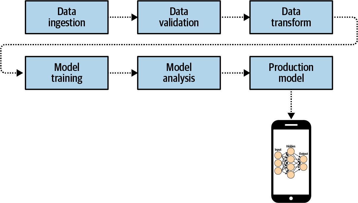
Figure 19-3. Deploying your production model to mobile

TensorFlow Serving fits into this architecture by providing the infrastructure for hosting your model on a server. Clients can then use HTTP to pass requests to this server along with a data payload. The data will be passed to the model, which will run inference, get the results, and return them to the client (Figure 19-4).

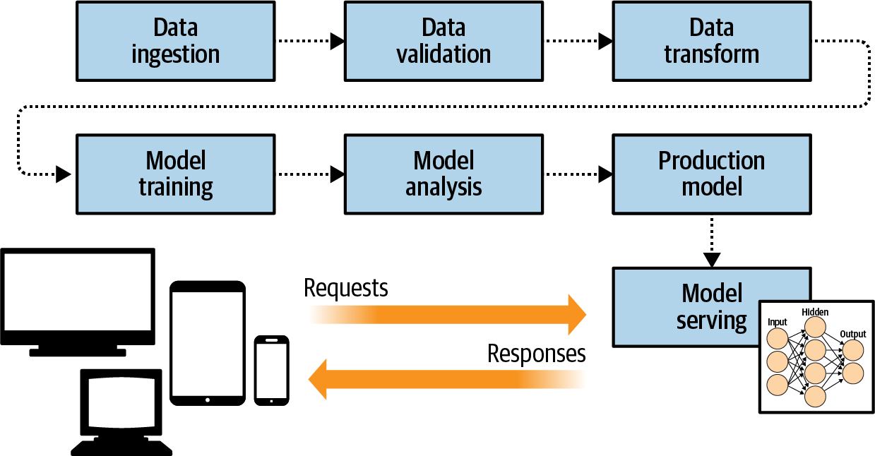
Figure 19-4. Adding model serving architecture to the pipeline

An important artifact of this type of architecture is that you can also control the versioning of the models used by your clients. When models are deployed to mobile devices, for example, you can end up with model drift, where different clients have different versions. But when serving from an infrastructure, as in Figure 19-4, you can avoid this. Additionally, this makes it possible to experiment with different model versions, where some clients will get the inference from one version of the model while others get it from other versions (Figure 19-5).

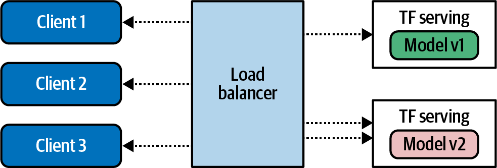
Figure 19-5. Using TensorFlow Serving to handle multiple model versions

Installing TensorFlow Serving

TensorFlow Serving can be installed with two different server architectures. The first, tensorflow-model-server, is a fully optimized server that uses platform-specific compiler options for various architectures. In general it’s the preferred option, unless your server machine doesn’t have those architectures. The alternative, tensorflow-model-server-universal, is compiled with basic optimizations that should work on all machines, and provides a nice backup if tensorflow-model-server does not work. There are several methods by which you can install TensorFlow Serving, including using Docker as well as a direct package installation using apt. We’ll look at both of those options next.

Installing Using Docker

Using Docker is perhaps the easiest way to get up and running quickly. To get started, use docker pull to get the TensorFlow Serving package:

docker pull tensorflow/serving

Once you’ve done this, clone the TensorFlow Serving code from GitHub:

git clone https://github.com/tensorflow/serving

This includes some sample models, including one called Half Plus Two that, given a value, will return half that value, plus two. To do this, first set up a variable called TESTDATA that contains the path of the sample models:

TESTDATA="$(pwd)/serving/tensorflow_serving/servables/tensorflow/testdata"

You can now run TensorFlow Serving from the Docker image:

docker run -t --rm -p 8501:8501 
    -v "$TESTDATA/saved_model_half_plus_two_cpu:/models/half_plus_two" 
    -e MODEL_NAME=half_plus_two 
    tensorflow/serving &

This will instantiate a server on port 8501—you’ll see how to do that in more detail later in this chapter—and execute the model on that server. You can then access the model at http://localhost:8501/v1/models/half_plus_two:predict.

To pass the data that you want to run inference on, you can POST a tensor containing the values to this URL. Here’s an example using curl (run this in a separate terminal if you’re running on your development machine) :

curl -d '{"instances": [1.0, 2.0, 5.0]}' 
    -X POST http://localhost:8501/v1/models/half_plus_two:predict

You can see the results in Figure 19-6.

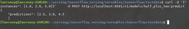
Figure 19-6. Results of running TensorFlow Serving

While the Docker image is certainly convenient, you might also want the full control of installing it directly on your machine. You’ll explore how to do that next.

apt-get remove tensorflow-model-server

echo "deb http://storage.googleapis.com/tensorflow-serving-apt stable
tensorflow-model-server tensorflow-model-server-universal" | tee
/etc/apt/sources.list.d/tensorflow-serving.list &&  curl
https://storage.googleapis.com/tensorflow-serving-apt/tensorflow-
serving.release.pub.gpg | apt-key add -

sudo echo "deb http://storage.googleapis.com/tensorflow-serving-apt stable
tensorflow-model-server tensorflow-model-server-universal" | sudo tee
/etc/apt/sources.list.d/tensorflow-serving.list &&  curl
https://storage.googleapis.com/tensorflow-serving-apt/tensorflow-
serving.release.pub.gpg | sudo apt-key add -

apt-get update

apt-get install tensorflow-model-server

apt-get upgrade tensorflow-model-server

Building and Serving a Model

In this section we’ll do a walkthrough of the complete process of creating a model, preparing it for serving, deploying it with TensorFlow Serving, and then running inference using it.

You’ll use the simple “Hello World” model that we’ve been exploring throughout the book:

xs = np.array([-1.0,  0.0, 1.0, 2.0, 3.0, 4.0], dtype=float)
ys = np.array([-3.0, -1.0, 1.0, 3.0, 5.0, 7.0], dtype=float)

model = tf.keras.Sequential([tf.keras.layers.Dense(units=1, input_shape=[1])])

model.compile(optimizer='sgd', loss='mean_squared_error')

history = model.fit(xs, ys, epochs=500, verbose=0)

print("Finished training the model")

print(model.predict([10.0]))

This should train very quickly and give you a result of 18.98 or so, when asked to predict Y when X is 10.0.

Next, the model needs to be saved. You’ll need a temporary folder to save it in:

import tempfile
import os
MODEL_DIR = tempfile.gettempdir()
version = 1
export_path = os.path.join(MODEL_DIR, str(version))
print(export_path)

When running in Colab, this should give you output like /tmp/1. If you’re running on your own system you can export it to whatever directory you want, but I like to use a temp directory.

If there’s anything in the directory you’re saving the model to, it’s a good idea to delete it before proceeding (avoiding this issue is one reason why I like using a temp directory!). To ensure that your model is the master, you can delete the contents of the export_path directory:

if os.path.isdir(export_path):
    print('
Already saved a model, cleaning up
')
    !rm -r {export_path}

Now you can save the model:

model.save(export_path, save_format="tf")

print('
export_path = {}'.format(export_path))
!ls -l {export_path}

Once this is done, take a look at the contents of the directory. The listing should show something like:

INFO:tensorflow:Assets written to: /tmp/1/assets

export_path = /tmp/1
total 48
drwxr-xr-x 2 root root  4096 May 21 14:40 assets
-rw-r--r-- 1 root root 39128 May 21 14:50 saved_model.pb
drwxr-xr-x 2 root root  4096 May 21 14:50 variables

The TensorFlow Serving tools include a utility called saved_model_cli that can be used to inspect a model. You can call this with the show command, giving it the directory of the model in order to get the full model metadata:

!saved_model_cli show --dir {export_path} --all

Note that the ! is used for Colab to indicate a shell command. If you’re using your own machine, it isn’t necessary.

The output of this command will be very long, but will contain details like this:

signature_def['serving_default']:
  The given SavedModel SignatureDef contains the following input(s):
    inputs['dense_input'] tensor_info:
        dtype: DT_FLOAT
        shape: (-1, 1)
        name: serving_default_dense_input:0
  The given SavedModel SignatureDef contains the following output(s):
    outputs['dense'] tensor_info:
        dtype: DT_FLOAT
        shape: (-1, 1)
        name: StatefulPartitionedCall:0

Note the content of the signature_def, which in this case is serving_default. You’ll need them later.

Also note that the inputs and outputs have a defined shape and type. In this case, each is a float and has the shape (–1, 1). You can effectively ignore the –1, and just bear in mind that the input to the model is a float and the output is a float.

If you are using Colab, you need to tell the operating system where the model directory is so that when you run TensorFlow Serving from a bash command, it will know the location. This can be done with an environment variable in the operating system:

os.environ["MODEL_DIR"] = MODEL_DIR

To run the TensorFlow model server with a command line, you need a number of parameters. First, you’ll use the --bg switch to ensure that the command runs in the background. The nohup command stands for “no hangup,” requesting that the script continues to run. Then you need to specify a couple of parameters to the tensorflow_model_server command. rest_api_port is the port number you want to run the server on. Here, it’s set to 8501. You then give the model a name with the model_name switch—here I’ve called it helloworld. Finally, you then pass the server the path to the model you saved in the MODEL_DIR operating system environment variable with model_base_path. Here’s the code:

%%bash --bg
nohup tensorflow_model_server 
  --rest_api_port=8501 
  --model_name=helloworld 
  --model_base_path="${MODEL_DIR}" >server.log 2>&1

At the end of the script is code to output the results to server.log. The output of this in Colab will simply be:

Starting job # 0 in a separate thread.

You can inspect it with:

!tail server.log

Examine this output, and you should see that the server started successfully with a note showing that it is exporting the HTTP/REST API at localhost:8501:

2020-05-21 14:41:20.026123: I tensorflow_serving/model_servers/server.cc:358]
Running gRPC ModelServer at 0.0.0.0:8500 ...
[warn] getaddrinfo: address family for nodename not supported
2020-05-21 14:41:20.026777: I tensorflow_serving/model_servers/server.cc:378]
Exporting HTTP/REST API at:localhost:8501 ...
[evhttp_server.cc : 238] NET_LOG: Entering the event loop ...

If it fails, you should see a notification about the failure. Should that happen, you might need to restart your system.

If you want to test the server, you can do so within Python:

import json
xs = np.array([[9.0], [10.0]])
data = json.dumps({"signature_name": "serving_default", "instances": 
    xs.tolist()})
print(data)

To send data to the server, you need to get it into JSON format. So with Python it’s a case of creating a Numpy array of the values you want to send—in this case it’s a list of two values, 9.0 and 10.0. Each of these is an array in itself, because as you saw earlier the input shape is (–1,1). Single values should be sent to the model, so if you want multiple ones it should be a list of lists, with the inner lists having single values only.

Use json.dumps in Python to create the payload, which is two name/value pairs. The first is the signature name to call on the model, which in this case is serving_default (as you’ll recall from earlier, when you inspected the model). The second is instances, which is the list of values you want to pass to the model.

Printing this will show you what the payload looks like:

{"signature_name": "serving_default", "instances": [[9.0], [10.0]]}

You can call the server using the requests library to do an HTTP POST. Note the URL structure. The model is called helloworld, and you want to run its prediction. The POST command requires data, which is the payload you just created, and a headers specification, where you’re telling the server the content type is JSON:

import requests
headers = {"content-type": "application/json"}
json_response = 
    requests.post('http://localhost:8501/v1/models/helloworld:predict', 
    data=data, headers=headers)

print(json_response.text)

The response will be a JSON payload containing the predictions:

{
    "predictions": [[16.9834747], [18.9806728]]
}

 model_config_list {
  config {
    name: '2x-1model'
    base_path: '/tmp/2xminus1/'
  }
  config {
    name: '3x+1model'
    base_path: '/tmp/3xplus1/'
  }
}

%%bash --bg
nohup tensorflow_model_server 
  --rest_api_port=8501 
  --model_config=/path/to/model.config >server.log 2>&1

model_config_list {
  config {
    name: '2x-1model'
    base_path: '/tmp/2xminus1/'
    model_version_policy: {
      specific {
        versions : 1
        versions : 2
      }
    }
  }
  config {
    name: '3x+1model'
    base_path: '/tmp/3xplus1/'
    model_version_policy: {
      all : {}
    }
  }
}

model_config_list {
  config {
    name: '2x-1model'
    base_path: '/tmp/2xminus1/'
    model_version_policy: {
      specific {
        versions : 1
        versions : 2
      }
    }
    version_labels {
      key: 'master'
      value: 1
    }
    version_labels {
      key: 'beta'
      value: 2
    }
  }
  config {
    name: '3x+1model'
    base_path: '/tmp/3xplus1/'
    model_version_policy: {
        all : {}
    }
  }
}

 <server>:8501/v1/models/2x-1model/versions/beta

%%bash --bg
nohup tensorflow_model_server 
  --rest_api_port=8501 
  --model_config=/path/to/model.config
  --model_config_file_poll_wait_seconds=60 >server.log 2>&1

Summary

In this chapter you had your first look at TensorFlow Extended (TFX). You saw that any machine learning system has components that go far beyond just building a model, and learned how one of those components—TensorFlow Serving, which provides model serving capabilities—can be installed and configured. You explored building a model, preparing it for serving, deploying it to a server, and then running inference using an HTTP POST request. After that you looked into the options for configuring your server with a configuration file, examining how to use it to deploy multiple models and different versions of those models. In the next chapter we’ll go in a different direction and see how distributed models can be managed for distributed learning while maintaining a user’s privacy with federated learning.