
Chapter 12. An Introduction to TensorFlow Lite
In all of the chapters of this book so far, you’ve been exploring how to use TensorFlow to create machine learning models that can provide functionality such as computer vision, natural language processing, and sequence modeling without the explicit programming of rules. Instead, using labeled data, neural networks are able to learn the patterns that distinguish one thing from another, and this can then be extended into solving problems. For the rest of the book we’re going to switch gears and look at how to use these models in common scenarios. The first, most obvious and perhaps most useful topic we’ll cover is how to use models in mobile applications. In this chapter, I’ll go over the underlying technology that makes it possible to do machine learning on mobile (and embedded) devices: TensorFlow Lite. Then, in the next two chapters we’ll explore scenarios of using these models on Android and iOS.
TensorFlow Lite is a suite of tools that complements TensorFlow, achieving two main goals. The first is to make your models mobile-friendly. This often involves reducing their size and complexity, with as little impact as possible on their accuracy, to make them work better in a battery-constrained environment like a mobile device. The second is to provide a runtime for different mobile platforms, including Android, iOS, mobile Linux (for example, Raspberry Pi), and various microcontrollers. Note that you cannot train a model with TensorFlow Lite. Your workflow will be to train it using TensorFlow and then convert it to the TensorFlow Lite format, before loading and running it using a TensorFlow Lite interpreter.
What Is TensorFlow Lite?
TensorFlow Lite started as a mobile version of TensorFlow aimed at Android and iOS developers, with the goal of being an effective ML toolkit for their needs. When building and executing models on computers or cloud services, issues like battery consumption, screen size, and other aspects of mobile app development aren’t a concern, so when mobile devices are targeted a new set of constraints need to be addressed.
The first is that a mobile application framework needs to be lightweight. Mobile devices have far more limited resources than the typical machine that is used for training models. As such, developers have to be very careful about the resources that are used not just by the application, but also the application framework. Indeed, when users are browsing an app store they’ll see the size of each application and have to make a decision about whether to download it based on their data usage. If the framework that runs a model is large, and the model itself is also large, this will bloat the file size and turn the user off.
The framework also has to be low latency. Apps that run on mobile devices need to perform well, or the user may stop using them. Only 38% of apps are used more than 11 times, meaning 62% of apps are used 10 times or less. Indeed, 25% of all apps are only used once. High latency, where an app is slow to launch or process key data, is a factor in this abandonment rate. Thus, a framework for ML-based apps needs to be fast to load and fast to perform the necessary inference.
In partnership with low latency, a mobile framework needs an efficient model format. When training on a powerful supercomputer, the model format generally isn’t the most important signal. As we’ve seen in earlier chapters, high model accuracy, low loss, avoiding overfitting, etc. are the metrics a model creator will chase. But when running on a mobile device, in order to be lightweight and have low latency, the model format will need to be taken into consideration as well. Much of the math in the neural networks we’ve seen so far is floating-point operations with high precision. For scientific discovery, that’s essential. For running on a mobile device it may not be. A mobile-friendly framework will need to help you with tradeoffs like this and give you the tools to convert your model if necessary.
Having your models run on-device has a major benefit in that they don’t need to pass data to a cloud service to have inference performed on it. This leads to improvements in user privacy as well as power consumption. Not needing to use the radio for a cellular or WiFi signal to send the data and receive the predictions is good, so long as the on-device inference doesn’t cost more power-wise. Keeping data on the device in order to run predictions is also a powerful and increasingly important feature, for obvious reasons! (Later in this book we’ll discuss federated learning, which is a hybrid of on-device and cloud-based machine learning that gives you the best of both worlds, while also maintaining privacy.)
So, with all of this in mind, TensorFlow Lite was created. As mentioned earlier, it’s not a framework for training models, but a supplementary set of tools designed to meet all the constraints of mobile and embedded systems.
It should broadly be seen as two main things: a converter that takes your TensorFlow model and converts it to the .tflite format, shrinking and optimizing it, and a suite of interpreters for various runtimes (Figure 12-1).
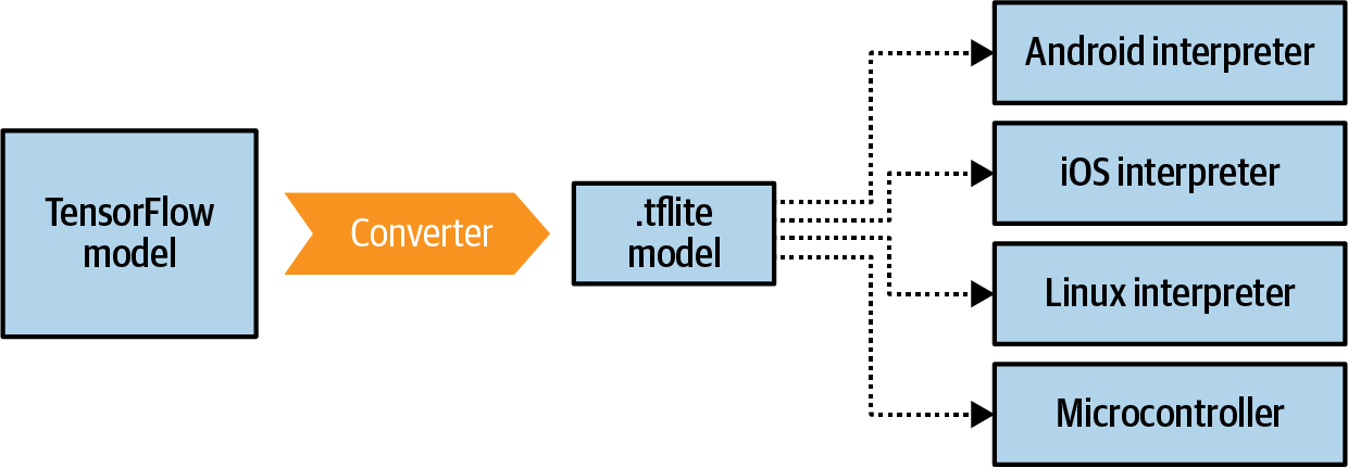
Figure 12-1. The TensorFlow Lite suite
The interpreter environments also support acceleration options within their particular frameworks. For example, on Android the Neural Networks API is supported, so TensorFlow Lite can take advantage of it on devices where it’s available.
Note that not every operation (or “op”) in TensorFlow is presently supported in TensorFlow Lite or the TensorFlow Lite converter. You may encounter this issue when converting models, and it’s always a good idea to check the documentation for details. One helpful piece of workflow, as you’ll see later in this chapter, is to take an existing mobile-friendly model and use transfer learning for your scenario. You can find lists of models optimized to work with TensorFlow Lite on the TensorFlow website and TensorFlow Hub.
Walkthrough: Creating and Converting a Model to TensorFlow Lite
We’ll begin with a step-by-step walkthrough showing how to create a simple model with TensorFlow, convert it to the TensorFlow Lite format, and then use the TensorFlow Lite interpreter. For this walkthrough I’ll use the Linux interpreter because it’s readily available in Google Colab. In Chapter 13 you’ll see how to use this model on Android, and in Chapter 14 you’ll explore using it on iOS.
Back in Chapter 1 you saw a very simple TensorFlow model that learned the relationship between two sets of numbers that ended up as Y = 2X – 1. For convenience, here’s the complete code:
l0=Dense(units=1,input_shape=[1])model=Sequential([l0])model.compile(optimizer='sgd',loss='mean_squared_error')xs=np.array([-1.0,0.0,1.0,2.0,3.0,4.0],dtype=float)ys=np.array([-3.0,-1.0,1.0,3.0,5.0,7.0],dtype=float)model.fit(xs,ys,epochs=500)(model.predict([10.0]))("Here is what I learned: {}".format(l0.get_weights()))
Once this has been trained, as you saw, you can do model.predict[x] and get the expected y. In the preceding code, x=10, and the y the model will give us back is a value close to 19.
As this model is small and easy to train, we can use it as an example that we’ll convert to TensorFlow Lite to show all the steps.
Step 1. Save the Model
The TensorFlow Lite converter works on a number of different file formats, including SavedModel (preferred) and the Keras H5 format. For this exercise we’ll use SavedModel.
Note
The TensorFlow team recommends using the SavedModel format for compatibility across the entire TensorFlow ecosystem, including future compatibility with new APIs.
To do this, simply specify a directory to save the model in and call tf.saved_model.save, passing it the model and directory:
export_dir='saved_model/1'tf.saved_model.save(model,export_dir)
The model will be saved out as assets and variables as well as a saved_model.pb file, as shown in Figure 12-2.
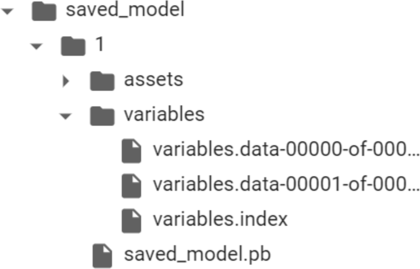
Figure 12-2. SavedModel structure
Once you have the saved model, you can convert it using the TensorFlow Lite converter.
Step 2. Convert and Save the Model
The TensorFlow Lite converter is in the tf.lite package. You can call it to convert a saved model by first invoking it with the from_saved_model method, passing it the directory containing the saved model, and then invoking its convert method:
# Convert the model.converter=tf.lite.TFLiteConverter.from_saved_model(export_dir)tflite_model=converter.convert()
You can then save out the new .tflite model using pathlib:
importpathlibtflite_model_file=pathlib.Path('model.tflite')tflite_model_file.write_bytes(tflite_model)
At this point you have a .tflite file that you can use in any of the interpreter environments. Later we’ll use it on Android and iOS, but for now, let’s use the Python-based interpreter so you can run it in Colab. This same interpreter can be used in embedded Linux environments like a Raspberry Pi!
Step 3. Load the TFLite Model and Allocate Tensors
The next step is to load the model into the interpreter, allocate tensors that will be used for inputting data to the model for prediction, and then read the predictions that the model outputs. This is where using TensorFLow Lite, from a programmer’s perspective, greatly differs from using TensorFlow. With TensorFlow you can just say model.predict(something) and get the results, but because TensorFlow Lite won’t have many of the dependencies that TensorFlow does, particularly in non-Python environments, you now have to get a bit more low-level and deal with the input and output tensors, formatting your data to fit them and parsing the output in a way that makes sense for your device.
First, load the model and allocate the tensors:
interpreter=tf.lite.Interpreter(model_content=tflite_model)interpreter.allocate_tensors()
Then you can get the input and output details from the model, so you can begin to understand what data format it expects and what data format it will provide back to you:
input_details=interpreter.get_input_details()output_details=interpreter.get_output_details()(input_details)(output_details)
You’ll get a lot of output!
First, let’s inspect the input parameter. Note the shape setting, which is an array of type [1,1]. Also note the class, which is numpy.float32. These settings will dictate the shape of the input data and its format:
[{'name':'dense_input','index':0,'shape':array([1,1],dtype=int32),'shape_signature':array([1,1],dtype=int32),'dtype':<class'numpy.float32'>,'quantization': (0.0,0),'quantization_parameters':{'scales':array([],dtype=float32),'zero_points':array([],dtype=int32),'quantized_dimension':0},'sparsity_parameters':{}}]
So, in order to format the input data, you’ll need to use code like this to define the input array shape and type if you want to predict the y for x=10.0:
to_predict=np.array([[10.0]],dtype=np.float32)(to_predict)
The double brackets around the 10.0 can cause a little confusion—the mnemonic I use for the array[1,1] here is to say that there is 1 list, giving us the first set of [], and that list contains just 1 value, which is [10.0], thus giving [[10.0]]. It can also be confusing that the shape is defined as dtype=int32, whereas you’re using numpy.float32. The dtype parameter is the data type defining the shape, not the contents of the list that is encapsulated in that shape. For that, you’ll use the class.
The output details are very similar, and what you want to keep an eye on here is the shape. As it’s also an array of type [1,1], you can expect the answer to be [[y]] in much the same way as the input was [[x]]:
[{'name':'Identity','index':3,'shape':array([1,1],dtype=int32),'shape_signature':array([1,1],dtype=int32),'dtype':<class'numpy.float32'>,'quantization': (0.0,0),'quantization_parameters':{'scales':array([],dtype=float32),'zero_points':array([],dtype=int32),'quantized_dimension':0},'sparsity_parameters':{}}]
Step 4. Perform the Prediction
To get the interpreter to do the prediction, you set the input tensor with the value to predict, telling it what input value to use:
interpreter.set_tensor(input_details[0]['index'],to_predict)interpreter.invoke()
The input tensor is specified using the index of the array of input details. In this case you have a very simple model that has only a single input option, so it’s input_details[0], and you’ll address it at the index. Input details item 0 has only one index, indexed at 0, and it expects a shape of [1,1] as defined earlier. So, you put the to_predict value in there. Then you invoke the interpreter with the invoke method.
You can then read the prediction by calling get_tensor and supplying it with the details of the tensor you want to read:
tflite_results=interpreter.get_tensor(output_details[0]['index'])(tflite_results)
Again, there’s only one output tensor, so it will be output_details[0], and you specify the index to get the details beneath it, which will have the output value.
So, for example, if you run this code:
to_predict=np.array([[10.0]],dtype=np.float32)(to_predict)interpreter.set_tensor(input_details[0]['index'],to_predict)interpreter.invoke()tflite_results=interpreter.get_tensor(output_details[0]['index'])(tflite_results)
you should see output like:
[[10.]][[18.975412]]
where 10 is the input value and 18.97 is the predicted value, which is very close to 19, which is 2X – 1 when X = 10. For why it’s not 19, look back to Chapter 1!
Given that this is a very simple example, let’s look at something a little more complex next—using transfer learning on a well-known image classification model, and then converting that for TensorFlow Lite. From there we’ll also be able to better explore the impacts of optimizing and quantizing the model.
Walkthrough: Transfer Learning an Image Classifier and Converting to TensorFlow Lite
In this section we’ll build a new version of the Dogs vs. Cats computer vision model from Chapters 3 and 4 that uses transfer learning. This will use a model from TensorFlow Hub, so if you need to install it, you can follow the instructions on the site.
Step 1. Build and Save the Model
First, get all of the data:
importnumpyasnpimportmatplotlib.pylabaspltimporttensorflowastfimporttensorflow_hubashubimporttensorflow_datasetsastfdsdefformat_image(image,label):image=tf.image.resize(image,IMAGE_SIZE)/255.0returnimage,label(raw_train,raw_validation,raw_test),metadata=tfds.load('cats_vs_dogs',split=['train[:80%]','train[80%:90%]','train[90%:]'],with_info=True,as_supervised=True,)num_examples=metadata.splits['train'].num_examplesnum_classes=metadata.features['label'].num_classes(num_examples)(num_classes)BATCH_SIZE=32train_batches=raw_train.shuffle(num_examples//4).map(format_image).batch(BATCH_SIZE).prefetch(1)validation_batches=raw_validation.map(format_image).batch(BATCH_SIZE).prefetch(1)test_batches=raw_test.map(format_image).batch(1)
This will download the Dogs vs. Cats dataset and split it into training, test, and validation sets.
Next, you’ll use the mobilenet_v2 model from TensorFlow Hub to create a Keras layer called feature_extractor:
module_selection=("mobilenet_v2",224,1280)handle_base,pixels,FV_SIZE=module_selectionMODULE_HANDLE="https://tfhub.dev/google/tf2-preview/{}/feature_vector/4".format(handle_base)IMAGE_SIZE=(pixels,pixels)feature_extractor=hub.KerasLayer(MODULE_HANDLE,input_shape=IMAGE_SIZE+(3,),output_shape=[FV_SIZE],trainable=False)
Now that you have the feature extractor, you can make it the first layer in your neural network and add an output layer with as many neurons as you have classes (in this case, two). You can then compile and train it:
model=tf.keras.Sequential([feature_extractor,tf.keras.layers.Dense(num_classes,activation='softmax')])model.compile(optimizer='adam',loss='sparse_categorical_crossentropy',metrics=['accuracy'])hist=model.fit(train_batches,epochs=5,validation_data=validation_batches)
With just five epochs of training, this should give a model with 99% accuracy on the training set and 98%+ on the validation set. Now you can simply save the model out:
CATS_VS_DOGS_SAVED_MODEL="exp_saved_model"tf.saved_model.save(model,CATS_VS_DOGS_SAVED_MODEL)
Once you have the saved model, you can convert it.
Step 2. Convert the Model to TensorFlow Lite
As before, you can now take the saved model and convert it into a .tflite model. You’ll save it out as converted_model.tflite:
converter=tf.lite.TFLiteConverter.from_saved_model(CATS_VS_DOGS_SAVED_MODEL)tflite_model=converter.convert()tflite_model_file='converted_model.tflite'withopen(tflite_model_file,"wb")asf:f.write(tflite_model)
Once you have the file, you can instantiate an interpreter with it. When this is done, you should get the input and output details as before. Load them into variables called input_index and output_index, respectively. This makes the code a little more readable!
interpreter=tf.lite.Interpreter(model_path=tflite_model_file)interpreter.allocate_tensors()input_index=interpreter.get_input_details()[0]["index"]output_index=interpreter.get_output_details()[0]["index"]predictions=[]
The dataset has lots of test images in test_batches, so if you want to take 100 of the images and test them, you can do so like this (feel free to change the 100 to any other value):
test_labels,test_imgs=[],[]forimg,labelintest_batches.take(100):interpreter.set_tensor(input_index,img)interpreter.invoke()predictions.append(interpreter.get_tensor(output_index))test_labels.append(label.numpy()[0])test_imgs.append(img)
Earlier, when reading the images, they were reformatted by the mapping function called format_image to be the right size for both training and inference, so all you have to do now is set the interpreter’s tensor at the input index to the image. After invoking the interpreter, you can then get the tensor at the output index.
If you want to see how the predictions did against the labels, you can run code like this:
score=0foriteminrange(0,99):prediction=np.argmax(predictions[item])label=test_labels[item]ifprediction==label:score=score+1("Out of 100 predictions I got"+str(score)+"correct")
This should give you a score of 99 or 100 correct predictions.
You can also visualize the output of the model against the test data with this code:
forindexinrange(0,99):plt.figure(figsize=(6,3))plt.subplot(1,2,1)plot_image(index,predictions,test_labels,test_imgs)plt.show()
You can see some of the results of this in Figure 12-3. (Note that all the code is available in the book’s GitHub repo, so if you need it, take a look there!)
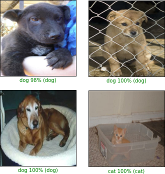
Figure 12-3. Results of inference
This is just the plain, converted model without any optimizations for mobile added. In the next step you’ll explore how to optimize this model for mobile devices.
Step 3. Optimize the Model
Now that you’ve seen the end-to-end process of training, converting, and using a model with the TensorFlow Lite interpreter, let’s look at how to get started with optimizing and quantizing the model.
The first type of optimization, called dynamic range quantization, is achieved by setting the optimizations property on the converter prior to performing the conversion. Here’s the code:
	converter = tf.lite.TFLiteConverter.from_saved_model(CATS_VS_DOGS_SAVED_MODEL)
converter.optimizations = [tf.lite.Optimize.DEFAULT]

tflite_model = converter.convert()
tflite_model_file = 'converted_model.tflite'

with open(tflite_model_file, "wb") as f:
    f.write(tflite_model)
There are several optimization options available at the time of writing (more may be added later). These include:
OPTIMIZE_FOR_SIZE- Perform optimizations that make the model as small as possible.
OPTIMIZE_FOR_LATENCY- Perform optimizations that reduce inference time as much as possible.
DEFAULT- Find the best balance between size and latency.
In this case, the model size was close to 9 MB before this step but only 2.3 MB afterwards—a reduction of almost 70%. Various experiments have shown that models can be made up to 4× smaller, with a 2–3× speedup. Depending on the model type, however, there can be a loss in accuracy, so it’s a good idea to test the model thoroughly if you quantize like this. In this case, I found that the accuracy of the model dropped from 99% to about 94%.
You can enhance this with full integer quantization or float16 quantization to take advantage of specific hardware. Full integer quantization changes the weights in the model from 32-bit floating point to 8-bit integer, which (particularly for larger models) can have a huge impact on model size and latency with a relatively small impact on accuracy.
To get full integer quantization, you’ll need to specify a representative dataset that tells the convertor roughly what range of data to expect. Update the code as follows:
	converter = tf.lite.TFLiteConverter.from_saved_model(CATS_VS_DOGS_SAVED_MODEL)

converter.optimizations = [tf.lite.Optimize.DEFAULT]

def representative_data_gen():
    for input_value, _ in test_batches.take(100):
        yield [input_value]

converter.representative_dataset = representative_data_gen
converter.target_spec.supported_ops = [tf.lite.OpsSet.TFLITE_BUILTINS_INT8]

tflite_model = converter.convert()
tflite_model_file = 'converted_model.tflite'

with open(tflite_model_file, "wb") as f:
    f.write(tflite_model)
Having this representative data allows the convertor to inspect data as it flows through the model and find where to best make the conversions. Then, by setting the supported ops (in this case to INT8), you can ensure that the precision of only those parts of the model is quantized. The result might be a slightly larger model—in this case, it went from 2.3 MB when using convertor.optimizations only to 2.8 MB. However, the accuracy went back up to 99%. Thus, by following these steps you can reduce the model’s size by about two-thirds, while maintaining its accuracy!
Summary
In this chapter you got an introduction to TensorFlow Lite and saw how it is designed to get your models ready for running on smaller, lighter devices than your development environment. These include mobile operating systems like Android, iOS, and iPadOS, as well as mobile Linux-based computing environments like the Raspberry Pi and microcontroller-based systems that support TensorFlow. You built a simple model and used it to explore the conversion workflow. You then worked through a more complex example, using transfer learning to retrain an existing model for your dataset, converting it to TensorFlow Lite, and optimizing it for a mobile environment. In the next chapter you’ll take this knowledge and explore how you can use the Android-based interpreter to use TensorFlow Lite in your Android apps!