Turning Sequences into Input Sequences

When predicting text, you need to train a neural network with an input sequence (feature) that has an associated label. Matching sequences to labels is the key to predicting text.

So, for example, if in your corpus you have the sentence “Today has a beautiful blue sky”, you could split this into ‘Today has a beautiful blue” as the feature and “sky” as the label. Then, if you were to get a prediction for the text “Today has a beautiful blue”, it would likely be “sky”. If in the training data you also have “Yesterday had a beautiful blue sky”, split in the same way, and you were to get a prediction for the text “Tomorrow will have a beautiful blue”, then there’s a high probability that the next word will be “sky”.

Given lots of sentences, training on sequences of words with the next word being the label, you can quickly build up a predictive model where the most likely next word in the sentence can be predicted from an existing body of text.

We’ll start with a very small corpus of text—an excerpt from a traditional Irish song from the 1860s, some of the lyrics of which are as follows:

Create a single string with all the text, and set that to be your data. Use for the line breaks. Then this corpus can be easily loaded and tokenized like this:

	tokenizer = Tokenizer()

data="In the town of Athy one Jeremy Lanigan 
 Battered away ... ..."
corpus = data.lower().split("
")

tokenizer.fit_on_texts(corpus)
total_words = len(tokenizer.word_index) + 1

The result of this process is to replace the words by their token values, as shown in Figure 8-1.

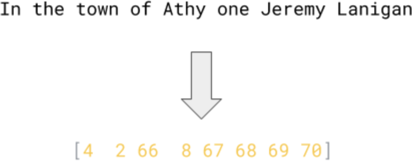
Figure 8-1. Tokenizing a sentence

To train a predictive model, we should take a further step here—splitting the sentence into multiple smaller sequences, so, for example, we can have one sequence consisting of the first two tokens, another of the first three, etc. (Figure 8-2).

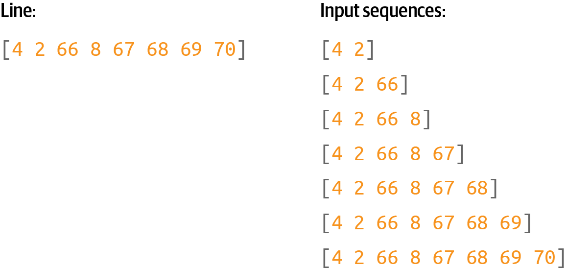
Figure 8-2. Turning a sequence into a number of input sequences

To do this you’ll need to go through each line in the corpus and turn it into a list of tokens using texts_to_sequences. Then you can split each list by looping through each token and making a list of all the tokens up to it.

Here’s the code:

	input_sequences = []
for line in corpus:
    token_list = tokenizer.texts_to_sequences([line])[0]
    for i in range(1, len(token_list)):
        n_gram_sequence = token_list[:i+1]
        input_sequences.append(n_gram_sequence)

print(input_sequences[:5])

Once you have these input sequences, you can pad them into a regular shape. We’ll use prepadding (Figure 8-3).

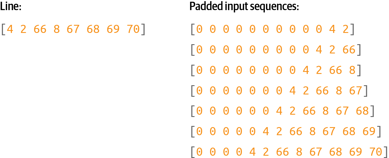
Figure 8-3. Padding the input sequences

To do this, you’ll need to find the longest sentence in the input sequences, and pad everything to that length. Here’s the code:

	max_sequence_len = max([len(x) for x in input_sequences])

input_sequences = np.array(pad_sequences(input_sequences, 
                            maxlen=max_sequence_len, padding='pre'))

Finally, once you have a set of padded input sequences, you can split these into features and labels, where the label is simply the last token in the input sequence (Figure 8-4).

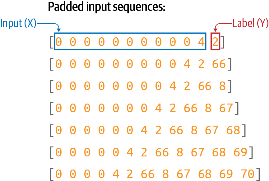
Figure 8-4. Turning the padded sequences into features (x) and labels (y)

When training a neural network, you’re going to match each feature to its corresponding label. So, for example, the label for [0 0 0 0 4 2 66 8 67 68 69] will be [70].

Here’s the code to separate the labels from the input sequences:

	xs, labels = input_sequences[:,:-1],input_sequences[:,-1]

Next, you need to encode the labels. Right now they’re just tokens—for example, the number 2 at the top of Figure 8-4. But if you want to use a token as a label in a classifier, it will have to be mapped to an output neuron. Thus, if you’re going to classify n words, with each word being a class, you’ll need to have n neurons. Here’s where it’s important to control the size of the vocabulary, because the more words you have, the more classes you’ll need. Remember back in Chapters 2 and 3 when you were classifying fashion items with the Fashion MNIST dataset, and you had 10 types of items of clothing? That required you to have 10 neurons in the output layer. In this case, what if you want to predict up to 10,000 vocabulary words? You’ll need an output layer with 10,000 neurons!

Additionally, you need to one-hot encode your labels so that they match the desired output from a neural network. Consider Figure 8-4. If a neural network is fed the input X consisting of a series of 0s followed by a 4, you’ll want the prediction to be 2, but how the network delivers that is by having an output layer of vocabulary_size neurons, where the second one has the highest probability.

To encode your labels into a set of Ys that you can then use to train, you can use the to_categorical utility in tf.keras:

ys = tf.keras.utils.to_categorical(labels, num_classes=total_words)

You can see this visually in Figure 8-5.

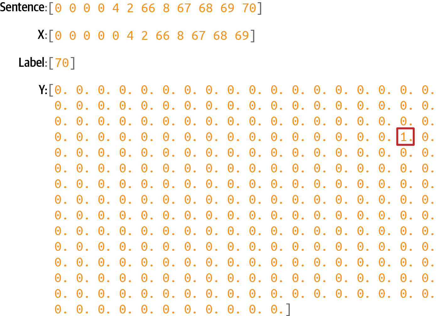
Figure 8-5. One-hot encoding labels

This is a very sparse representation, which, if you have a lot of training data and a lot of potential words, will eat memory very quickly! Suppose you had 100,000 training sentences, with a vocabulary of 10,000 words—you’d need 1,000,000,000 bytes just to hold the labels! But it’s the way we have to design our network if we’re going to classify and predict words.

Creating the Model

Let’s now create a simple model that can be trained with this input data. It will consist of just an embedding layer, followed by an LSTM, followed by a dense layer.

For the embedding you’ll need one vector per word, so the parameters will be the total number of words and the number of dimensions you want to embed on. In this case we don’t have many words, so eight dimensions should be enough.

You can make the LSTM bidirectional, and the number of steps can be the length of a sequence, which is our max length minus 1 (because we took one token off the end to make the label).

Finally, the output layer will be a dense layer with the total number of words as a parameter, activated by softmax. Each neuron in this layer will be the probability that the next word matches the word for that index value:

	model = Sequential()
model.add(Embedding(total_words, 8))
model.add(Bidirectional(LSTM(max_sequence_len-1)))
model.add(Dense(total_words, activation='softmax'))

Compile the model with a categorical loss function such as categorical cross entropy and an optimizer like Adam. You can also specify that you want to capture metrics:

	model.compile(loss='categorical_crossentropy', 
               optimizer='adam', metrics=['accuracy'])

It’s a very simple model without a lot of data, so you can train for a long time—say, 1,500 epochs:

	history = model.fit(xs, ys, epochs=1500, verbose=1)

After 1,500 epochs, you’ll see that it has reached very high accuracy (Figure 8-6).

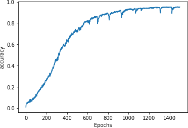
Figure 8-6. Training accuracy

With the model at around 95% accuracy, we can be assured that if we have a string of text that it has already seen it will predict the next word accurately about 95% of the time. Note, however, that when generating text it will continually see words that it hasn’t previously seen, so despite this good number, you’ll find that the network will rapidly end up producing nonsensical text. We’ll explore this in the next section.

Generating Text

Now that you’ve trained a network that can predict the next word in a sequence, the next step is to give it a sequence of text and have it predict the next word. Let’s take a look at how to do that.

	seed_text = "in the town of athy"

	token_list = tokenizer.texts_to_sequences([seed_text])[0]

	token_list = pad_sequences([token_list], 
                            maxlen=max_sequence_len-1, padding='pre')

	predicted = np.argmax(model.predict(token_list), axis=-1)
print(predicted)

	'town': 66, 'athy': 67, 'one': 68, 'jeremy': 69, 'lanigan': 70,

	for word, index in tokenizer.word_index.items():
    if index == predicted:
        print(word)
        break

	seed_text = "sweet jeremy saw dublin"
next_words=10

for _ in range(next_words):
    token_list = tokenizer.texts_to_sequences([seed_text])[0]
    token_list = pad_sequences([token_list], 
 maxlen=max_sequence_len-1, padding='pre')
    predicted = model.predict_classes(token_list, verbose=0)
    output_word = ""


    for word, index in tokenizer.word_index.items():
        if index == predicted:
            output_word = word
            break
    seed_text += " " + output_word

print(seed_text)

sweet jeremy saw dublin then got there as me me a call doing me

Extending the Dataset

The same pattern that you used for the hardcoded dataset can be extended to use a text file very simply. I’ve hosted a text file containing about 1,700 lines of text gathered from a number of songs that you can use for experimentation. With a little modification, you can use this instead of the single hardcoded song.

To download the data in Colab, use the following code:

	!wget --no-check-certificate 
    https://storage.googleapis.com/laurencemoroney-blog.appspot.com/irish-lyrics-eof.txt 
    -O /tmp/irish-lyrics-eof.txt

Then you can simply load the text from it into your corpus like this:

	data = open('/tmp/irish-lyrics-eof.txt').read()
corpus = data.lower().split("
")

The rest of your code will then work without modification!

Training this for 1,000 epochs brings you to about 60% accuracy, with the curve flattening out (Figure 8-7).

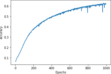
Figure 8-7. Training on a larger dataset

Trying the phrase “in the town of athy” again yields a prediction of “one”, but this time with only a 40% probability.

For “sweet jeremy saw dublin” the predicted next word is “drawn”, with a probability of 59%. Predicting the next 10 words yields:

sweet jeremy saw dublin drawn and fondly i am dead and the parting graceful

It’s looking a little better! But can we improve it further?

Changing the Model Architecture

One way that you can improve the model is to change its architecture, using multiple stacked LSTMs. This is pretty straightforward—just ensure that you set return_sequences to True on the first of them. Here’s the code:

	model = Sequential()
model.add(Embedding(total_words, 8))
model.add(Bidirectional(LSTM(max_sequence_len-1, return_sequences='True')))
model.add(Bidirectional(LSTM(max_sequence_len-1)))
model.add(Dense(total_words, activation='softmax'))
model.compile(loss='categorical_crossentropy', optimizer='adam', metrics=['accuracy'])
history = model.fit(xs, ys, epochs=1000, verbose=1)

You can see the impact this has on training for 1,000 epochs in Figure 8-8. It’s not significantly different from the previous curve.

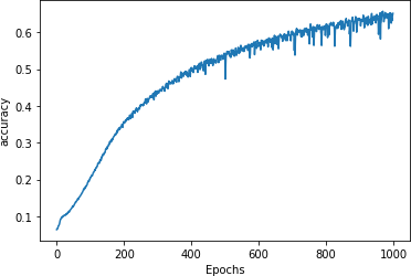
Figure 8-8. Adding a second LSTM layer

When testing with the same phrases as before, this time I got “more” as the next word after “in the town of athy” with a 51% probability, and after “sweet jeremy saw dublin” I got “cailín” (the Gaelic word for “girl”) with a 61% probability. Again, when predicting more words, the output quickly descended into gibberish.

Here are some examples:

	sweet jeremy saw dublin cailín loo ra fountain plundering that fulfill you mccarthy you mccarthy down

you know nothing jon snow johnny cease and she danced that put to smother well i must the wind flowers
dreams it love to laid ned the mossy and night i weirs

If you get different results, don’t worry—you didn’t do anything wrong, but the random initialization of the neurons will impact the final scores.

Improving the Data

There’s a small trick that you can use to extend the size of this dataset without adding any new songs, called windowing the data. Right now, every line in every song is read as a single line and then turned into input sequences, as you saw in Figure 8-2. While humans read songs line by line in order to hear rhyme and meter, the model doesn’t have to, in particular when using bidirectional LSTMs.

So, instead of taking the line “In the town of Athy, one Jeremy Lanigan”, processing that, and then moving to the next line (“Battered away till he hadn’t a pound”) and processing that, we could treat all the lines as one long, continuous text. We can then create a “window” into that text of n words, process that, and then move the window forward one word to get the next input sequence (Figure 8-9).

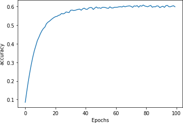
Figure 8-9. A moving word window

In this case, far more training data can be yielded in the form of an increased number of input sequences. Moving the window across the entire corpus of text would give us ((number_of_words – window_size) ✕ window_size) input sequences that we could train with.

The code is pretty simple—when loading the data, instead of splitting each song line into a “sentence,” we can create them on the fly from the words in the corpus:

	window_size=10
sentences=[]
alltext=[]
data = open('/tmp/irish-lyrics-eof.txt').read()
corpus = data.lower()
words = corpus.split(" ")
range_size = len(words)-max_sequence_len
for i in range(0, range_size):
    thissentence=""
    for word in range(0, window_size-1):
        word = words[i+word]
        thissentence = thissentence + word
        thissentence = thissentence + " "
    sentences.append(thissentence)

In this case, because we no longer have sentences and we’re creating sequences the same size as the moving window, max_sequence_len is the size of the window. The full file is read, converted to lowercase, and split into an array of words using string splitting. The code then loops through the words and makes sentences of each word from the current index up to the current index plus the window size, adding each of those newly constructed sentences to the sentences array.

When training you’ll notice that the extra data makes it much slower per epoch, but the results are greatly improved, and the generated text descends into gibberish much more slowly. Here’s an example that caught my eye—particularly the last line!

• you know nothing, jon snow is gone

• and the young and the rose and wide

• to where my love i will play

• the heart of the kerry

• the wall i watched a neat little town

There are many hyperparameters you can try tuning. Changing the window size will change the amount of training data—a smaller window size can yield more data, but there will be fewer words to give to a label, so if you set it too small you’ll end up with nonsensical poetry. You can also change the dimensions in the embedding, the number of LSTMs, or the size of the vocab to use for training. Given that percentage accuracy isn’t the best measurement—you’ll want to make a more subjective examination of how much “sense” the poetry makes—there’s no hard-and-fast rule to follow to determine whether your model is “good” or not.

For example, when I tried using a window size of 6, increasing the number of dimensions for the embedding to 16, changing the number of LSTMs from the window size (which would be 6) to 32, and upping the learning rate on the Adam optimizer, I got a nice, smooth, learning curve (Figure 8-10) and some of the poetry began to make more sense.

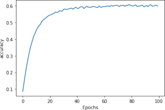
Figure 8-10. Learning curve with adjusted hyperparameters

When using “sweet jeremy saw dublin” as the seed (remember, all of the words in the seed are in the corpus), I got this poem:

• sweet jeremy saw dublin

• whack fol

• all the watch came

• and if ever you love get up from the stool

• longs to go as i was passing my aged father

• if you can visit new ross

• gallant words i shall make

• such powr of her goods

• and her gear

• and her calico blouse

• she began the one night

• rain from the morning so early

• oer railroad ties and crossings

• i made my weary way

• through swamps and elevations

• my tired feet

• was the good heavens

While the phrase “whack fol” may not make sense to many readers, it’s commonly heard in some Irish songs, kind of like “la la la” or “doobie-doobie-doo”. What I really liked about this was how some of the later phrases kept some kind of sense, like “such power of her good and her gear, and her calico blouse”—but this could be due to overfitting to the phrases that already exist in the songs within the corpus. For example, the lines beginning “oer railroad ties…” through “my tired feet” are taken directly from a song called “The Lakes of Pontchartrain” which is in the corpus. If you encounter issues like this, it’s best to reduce the learning rate and maybe decrease the number of LSTMs. But above all, experiment and have fun!

Character-Based Encoding

For the last few chapters we’ve been looking at NLP using word-based encoding. I find that much easier to get started with, but when it comes to generating text, you might also want to consider character-based encoding because the number of unique characters in a corpus tends to be a lot less than the number of unique words. As such, you can have a lot fewer neurons in your output layer, and your output predictions are spread across fewer probabilities. For example, when looking at the dataset of the complete works of Shakespeare, you’ll see that there are only 65 unique characters in the entire set. So, when you are making predictions, instead of looking at probabilities of the next word across 2,700 words as in the Irish songs dataset, you’re only looking at 65. This makes your model a bit simpler!

What’s also nice about character encoding is that punctuation characters are also included, so line breaks etc. can be predicted. As an example, when I used an RNN trained on the Shakespeare corpus to predict the text following on from my favorite Game of Thrones line, I got:

• YGRITTE: You know nothing, Jon Snow.

• Good night, we’ll prove those body’s servants to

• The traitor be these mine:

• So diswarl his body in hope in this resceins,

• I cannot judg appeal’t.

• MENENIUS:

• Why, ’tis pompetsion.

• KING RICHARD II:

• I think he make her thought on mine;

• She will not: suffer up thy bonds:

• How doched it, I pray the gott,

• We’ll no fame to this your love, and you were ends

It’s kind of cool that she identifies him as a traitor and wants to tie him up (“diswarl his body”), but I have no idea what “resceins” means! If you watch the show, this is part of the plot, so maybe Shakespeare was on to something without realizing it!

Of course, I do think we tend to be a little more forgiving when using something like Shakespeare’s texts as our training data, because the language is already a little unfamiliar.

As with the Irish songs model the output does quickly degenerate into nonsensical text, but it’s still fun to play with. To try it for yourself, you can check out the Colab.

Summary

In this chapter we explored how to do basic text generation using a trained LSTM-based model. You saw how you can split text into training features and labels, using words as labels, and create a model that, when given seed text, can predict the next likely word. You iterated on this to improve the model for better results, exploring a dataset of traditional Irish songs. You also saw a little about how this could potentially be improved with character-based text generation with an example that uses Shakespearian text. Hopefully this was a fun introduction to how machine learning models can synthesize text!