
Chapter 17. Reusing and Converting Python Models to JavaScript
While training in the browser is a powerful option, you may not always want to do this because of the time involved. As you saw in Chapter 15 and Chapter 16, even training simple models can lock up the browser for some time. Having a visualization of the progress helped, but it still wasn’t the best of experiences. There are three alternatives to this approach. The first is to train models in Python and convert them to JavaScript. The second is to use existing models that were trained elsewhere and are provided in a JavaScript-ready format. The third is to use transfer learning, introduced in Chapter 3. In that case, features, weights, or biases that have been learned in one scenario can be transferred to another, instead of doing time-consuming relearning. We’ll cover the first two cases in this chapter, and then in Chapter 18 you’ll see how to do transfer learning in JavaScript.
Converting Python-Based Models to JavaScript
Models that have been trained using TensorFlow may be converted to JavaScript using the Python-based tensorflowjs tools. You can install these using:
!pip install tensorflowjs
For example, consider the following simple model that we’ve been using throughout the book:
import numpy as np
import tensorflow as tf
from tensorflow.keras import Sequential
from tensorflow.keras.layers import Dense

l0 = Dense(units=1, input_shape=[1])
model = Sequential([l0])
model.compile(optimizer='sgd', loss='mean_squared_error')

xs = np.array([-1.0, 0.0, 1.0, 2.0, 3.0, 4.0], dtype=float)
ys = np.array([-3.0, -1.0, 1.0, 3.0, 5.0, 7.0], dtype=float)

model.fit(xs, ys, epochs=500, verbose=0)

print(model.predict([10.0]))
print("Here is what I learned: {}".format(l0.get_weights()))
The trained model can be saved as a saved model with this code:
tf.saved_model.save(model, '/tmp/saved_model/')
Once you have the saved model directory, you can then use the TensorFlow.js converter by passing it an input format—which in this case is a saved model—along with the location of the saved model directory and the desired location for the JSON model:
!tensorflowjs_converter
    --input_format=keras_saved_model
    /tmp/saved_model/
    /tmp/linear
The JSON model will be created in the specified directory (in this case, /tmp/linear). If you look at the contents of this directory, you’ll also see a binary file, in this case called group1-shardof1.bin (Figure 17-1). This file contains the weights and biases that were learned by the network in an efficient binary format.
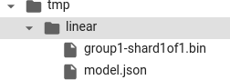
Figure 17-1. The output of the JS converter
The JSON file contains text describing the model. For example, within the JSON file you’ll see a setting like this:
"weightsManifest": [
   {"paths": ["group1-shard1of1.bin"],
    "weights": [{"name": "dense_2/kernel", "shape": [1, 1], "dtype": "float32"},
  {"name": "dense_2/bias", "shape": [1], "dtype": "float32"}]}
]}
This indicates the location of the .bin file holding the weights and biases, and their shape.
If you examine the contents of the .bin file in a hex editor, you’ll see that there are 8 bytes in it (Figure 17-2).
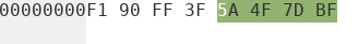
Figure 17-2. The bytes in the .bin file
As our network learned with a single neuron to get Y = 2X – 1, the network learned a single weight as a float32 (4 bytes), and a single bias as a float32 (4 bytes). Those 8 bytes are written to the .bin file.
If you look back to the output from the code:
Here is what I learned: [array([[1.9966108]], dtype=float32),
array([-0.98949206], dtype=float32)]
you can then convert the weight (1.9966108) to hexadecimal using a tool like the Floating Point to Hex Converter (Figure 17-3).
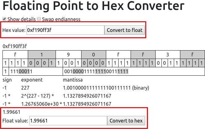
Figure 17-3. Converting the float value to hex
You can see that the weight of 1.99661 was converted to hex of F190FF3F, which is the value of the first 4 bytes in the hex file from Figure 17-2. You’ll see a similar result if you convert the bias to hex (note that you’ll need to swap endianness).
Using the Converted Models
One you have the JSON file and its associated .bin file, you can use them in a TensorFlow.js app easily. To load the model from the JSON file, you specify a URL where it’s hosted. If you’re using the built-in server from Brackets, it will be at 127.0.0.1:<port>. When you specify this URL, you can load the model with await tf.loadLayersModel(URL). Here’s an example:
const MODEL_URL = 'http://127.0.0.1:35601/model.json';
const model = await tf.loadLayersModel(MODEL_URL);
You might need to change the 35601 to your local server port. The model.json file and the .bin file need to be in the same directory.
If you want to run a prediction using the model, you use a tensor2d as before, passing the input value and its shape. So, in this case, if you want to predict the value of 10.0, you can create a tensor2d containing [10.0] as the first parameter and [1,1] as the second:
const input = tf.tensor2d([10.0], [1, 1]);
const result = model.predict(input);
For convenience, here’s the entire HTML page for this model:
<html>
<head>
<script src="https://cdn.jsdelivr.net/npm/@tensorflow/tfjs@latest"></script>
<script>
    async function run(){
        const MODEL_URL = 'http://127.0.0.1:35601/model.json';
        const model = await tf.loadLayersModel(MODEL_URL);
        console.log(model.summary());
        const input = tf.tensor2d([10.0], [1, 1]);
        const result = model.predict(input);
        alert(result);
    }
    run();
</script>
<body>
</body>
</html>
When you run the page, it will instantly load the model and alert the results of the prediction. You can see this in Figure 17-4.
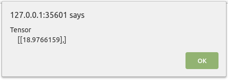
Figure 17-4. Output from the inference
Obviously this was a very simple example, where the model binary file was only 8 bytes and easy to inspect. However, hopefully it was useful to help you understand how the JSON and binary representations go hand-in-hand. As you convert your own models you’ll see much larger binary files—which ultimately are just the binary encoded weights and biases from your model, as you saw here.
In the next section you’ll look at some models that have already been converted for you using this method, and how you can use them in JavaScript.
Using Preconverted JavaScript Models
In addition to being able to convert your models to JavaScript, you can also use preconverted models. The TensorFlow team has created several of these for you to try, which you can find on GitHub. There are models available for different data types, including images, audio, and text. Let’s explore some of these models and how you can use them in JavaScript.
Using the Toxicity Text Classifier
One of the text-based models provided by the TensorFlow team is the Toxicity classifier. This takes in a text string and predicts whether it contains one of the following types of toxicity:
Identity attack
Insult
Obscenity
Severe toxicity
Sexually explicit
Threat
General toxicity
It’s trained on the Civil Comments dataset, containing over 2 million comments that have been labeled according to these types. Using it is straightforward. You can load the model alongside TensorFlow.js like this:
<script src="https://cdn.jsdelivr.net/npm/@tensorflow/tfjs@latest"></script>
<script src="https://cdn.jsdelivr.net/npm/@tensorflow-models/toxicity"></script>
Once you have the libraries, you can set a threshold value above which the sentences will be classified. It defaults to 0.85, but you can change it to something else like this, specifying it when you load the model:
const threshold = 0.7;
toxicity.load(threshold).then(model => {
Then, if you want to classify a sentence, you can put it in an array. Multiple sentences can be classified simultaneously:
const sentences = ['you suck', 'I think you are stupid',
                    'i am going to kick your head in',
                   'you feeling lucky, punk?'];

model.classify(sentences).then(predictions => {
At this point you can parse the predictions object for the results. It will be an array with seven entries, one for each of the toxicity types (Figure 17-5).
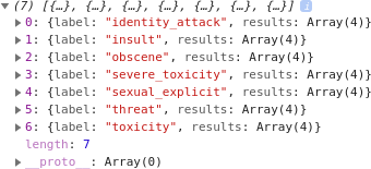
Figure 17-5. The results of a toxicity prediction
Within each of these are the results for each sentence against that class. So, for example, if you look at item 1, for insults, and expand it to explore the results, you’ll see that there are four elements. These are the probabilities for that type of toxicity for each of the four input sentences (Figure 17-6).
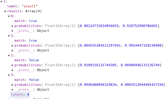
Figure 17-6. Exploring toxicity results
The probabilities are measured as [negative, positive], so a high value in the second element indicates that type of toxicity is present. In this case, the sentence “you suck” was measured as having a .91875 probability of being an insult, whereas “I am going to kick your head in,” while toxic, shows a low level of insult probability at 0.089.
To parse these out, you can loop through the predictions array, loop through each of the insult types within the results, and then loop through their results in order to find the types of toxicity identified in each sentence. You can do this by using the match method, which will be positive if the predicted value is above the threshold.
Here’s the code:
for(sentence=0; sentence<sentences.length; sentence++){
  for(toxic_type=0; toxic_type<7; toxic_type++){
    if(predictions[toxic_type].results[sentence].match){
      console.log("In the sentence: " + sentences[sentence] + "
" +
                   predictions[toxic_type].label +
                   " was found with probability of " +
                   predictions[toxic_type].results[sentence].probabilities[1]);
    }
  }
}
You can see the results of this in Figure 17-7.
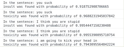
Figure 17-7. Results of the Toxicity classifier on the sample input
So, if you wanted to implement some kind of toxicity filter on your site, you could do so with very few lines of code like this!
One other useful shortcut is that if you don’t want to catch all seven forms of toxicity, you can specify a subset like this:
const labelsToInclude = ['identity_attack', 'insult', 'threat'];
and then specify this list alongside the threshold when loading the model:
toxicity.load(threshold, labelsToInclude).then(model => {}
The model, of course, can also be used with a Node.js backend if you want to capture and filter toxicity on the backend.
Using MobileNet for Image Classification in the Browser
As well as text classification libraries, the repository includes some libraries for image classification, such as MobileNet. MobileNet models are designed to be small and power-friendly while also accurate at classifying 1,000 classes of image. As a result, they have 1,000 output neurons, each of which is a probability that the image contains that class. So, when you pass an image to the model, you’ll get back a list of 1,000 probabilities that you’ll need to map to these classes. However, the JavaScript library abstracts this for you, picking the top three classes in order of priority and providing just those.
Here’s an excerpt from the full list of classes:
00: background
01: tench
02: goldfish
03: great white shark
04: tiger shark
05: hammerhead
06: electric ray
To get started, you need to load the TensorFlow.js and mobilenet scripts, like this:
<script src="https://cdn.jsdelivr.net/npm/@tensorflow/tfjs@latest"> </script>
<script src="https://cdn.jsdelivr.net/npm/@tensorflow-models/[email protected]">
To use the model, you need to provide it with an image. The simplest way to do this is to create an <img> tag and load an image into it. You can also create a <div> tag to hold the output:
<body>
    <img id="img" src="coffee.jpg"></img>
    <div id="output" style="font-family:courier;font-size:24px;height=300px">
    </div>
</body>
To use the model to classify the image, you then simply load it and pass a reference to the <img> tag to the classifier:
const img = document.getElementById('img');
const outp = document.getElementById('output');
mobilenet.load().then(model => {
    model.classify(img).then(predictions => {
        console.log(predictions);
    });
});
This prints the output to the console log, which will look like Figure 17-8.
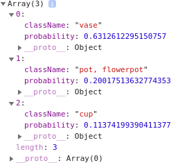
Figure 17-8. Exploring the MobileNet output
The output, as a prediction object, can also be parsed, so you can iterate through it and pick out the class name and probability like this:
for(var i = 0; i<predictions.length; i++){
    outp.innerHTML += "<br/>" + predictions[i].className + " : "
     + predictions[i].probability;
}
Figure 17-9 shows the sample image in the browser alongside the predictions.

Figure 17-9. Classifying an image
For convenience, here’s the entire code listing for this simple page. To use it you need to have an image in the same directory. I’m using coffee.jpg, but you can of course replace the image and change the src attribute of the <img> tag to classify something else:
<html>
<head>
<script src="https://cdn.jsdelivr.net/npm/@tensorflow/tfjs@latest"> </script>
<script src="https://cdn.jsdelivr.net/npm/@tensorflow-models/[email protected]"> </script>
</head>
<body>
    <img id="img" src="coffee.jpg"></img>
    <div id="output" style="font-family:courier;font-size:24px;height=300px">
    </div>
</body>
<script>
    const img = document.getElementById('img');
    const outp = document.getElementById('output');
    mobilenet.load().then(model => {
        model.classify(img).then(predictions => {
            console.log(predictions);
            for(var i = 0; i<predictions.length; i++){
                outp.innerHTML += "<br/>" + predictions[i].className + " : "
                + predictions[i].probability;
            }
        });
    });
</script>
</html>
Using PoseNet
Another interesting library that has been preconverted for you by the TensorFlow team is PoseNet, which can give you near-real-time pose estimation in the browser. It takes an image and returns a set of points for 17 body landmarks in the image. These are:
Nose
Left and right eye
Left and right ear
Left and right shoulder
Left and right elbow
Left and right wrist
Left and right hip
Left and right knee
Left and right ankle
For a simple scenario, we can look at estimating the pose for a single image in the browser. To do this, first, load TensorFlow.js and the posenet model:
<head>
    <script src="https://cdn.jsdelivr.net/npm/@tensorflow/tfjs"></script>
    <script src="https://cdn.jsdelivr.net/npm/@tensorflow-models/posenet">
    </script>
</head>
In the browser, you can load the image into an <img> tag and create a canvas on which you can draw the locations of the body landmarks:
<div><canvas id='cnv' width='661px' height='656px'/></div>
<div><img id='master' src="tennis.png"/></div>
To get the predictions, you can then just get the image element containing the picture and pass it to posenet, calling the estimateSinglePose method:
var imageElement = document.getElementById('master');
posenet.load().then(function(net) {
    const pose = net.estimateSinglePose(imageElement, {});
    return pose;
}).then(function(pose){
    console.log(pose);
    drawPredictions(pose);
})
This will return the predictions in an object called pose. This is an array of keypoints of the body parts (Figure 17-10).
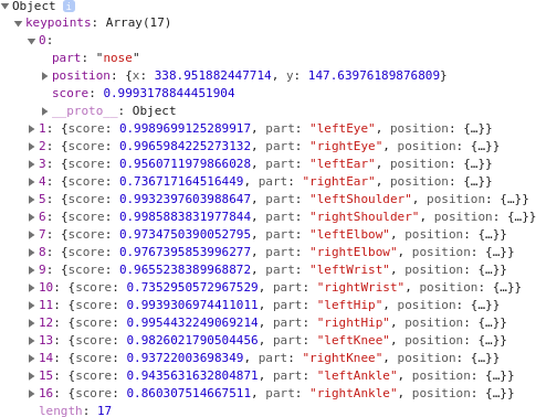
Figure 17-10. The returned positions for the pose
Each item contains a text description of the part (e.g., nose), an object with the x and y coordinates of the position, and a score value indicating the confidence that the landmark was correctly spotted. So, for example, in Figure 17-10, the likelihood that the landmark nose was spotted is .999.
You can then use these to plot the landmarks on the image. First load the image into the canvas, and then you can draw on it:
var canvas = document.getElementById('cnv');
var context = canvas.getContext('2d');
var img = new Image()
img.src="tennis.png"
img.onload = function(){
    context.drawImage(img, 0, 0)
    var centerX = canvas.width / 2;
    var centerY = canvas.height / 2;
    var radius = 2;
You can then loop through the predictions, retrieving the part names and (x,y) coordinates, and plot them on the canvas with this code:
for(i=0; i<pose.keypoints.length; i++){
    part = pose.keypoints[i].part
    loc = pose.keypoints[i].position;
    context.beginPath();
    context.font = "16px Arial";
    context.fillStyle="aqua"
    context.fillText(part, loc.x, loc.y)
    context.arc(loc.x, loc.y, radius, 0, 2 * Math.PI, false);
    context.fill();
}
Then, at runtime, you should see something like Figure 17-11.
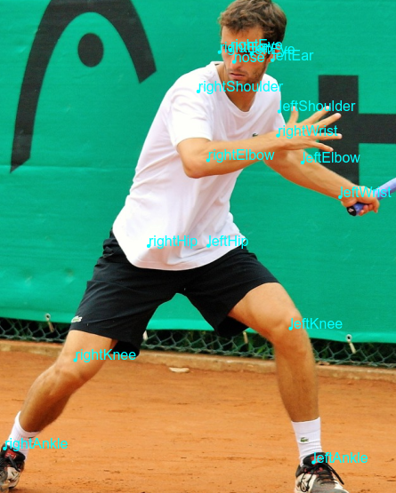
Figure 17-11. Estimating and drawing body part positions on an image
You can also use the score property to filter out bad predictions. For example, if your picture only contains a person’s face, you can update the code to filter out the low-probability predictions in order to focus on just the relevant landmarks:
for(i=0; i<pose.keypoints.length; i++){
    if(pose.keypoints[i].score>0.1){
    // Plot the points
    }
}
If the image is a closeup of somebody’s face, you don’t want to plot shoulders, ankles, etc. These will have very low but nonzero scores, so if you don’t filter them out they’ll be plotted somewhere on the image—and as the image doesn’t contain these landmarks, this will clearly be an error!
Figure 17-12 shows a picture of a face with low-probability landmarks filtered out. Note that there is no mouth landmark as PoseNet is primarily intended for estimating body poses, not faces.
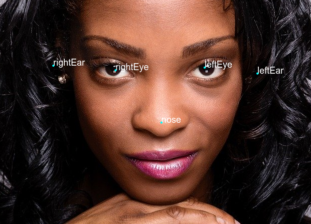
Figure 17-12. Using PoseNet on a face
There are many more features available in the PoseNet model—we’ve barely scratched the surface of what’s possible. You can do real-time pose detection in the browser with the webcam, edit the accuracy of the poses (lower-accuracy predictions can be faster), choose the architecture to optimize for speed, detect poses for multiple bodies, and much more.
Summary
In this chapter you saw how you can use TensorFlow.js with Python-created models, either by training your own model and converting it with the provided tools or by using preexisting models. When converting, you saw how the tensorflowjs tools created a JSON file with the metadata of your model as well as a binary file containing the weights and biases. It was easy to import your model as a JavaScript library and use it directly in the browser.
You then looked at a few examples of existing models that have been converted for you, and how you can incorporate them into your JavaScript code. You first experimented with the Toxicity model for processing text to identify and filter out toxic comments. You then explored using the MobileNet model for computer vision to predict the contents of an image. Finally, you saw how to use the PoseNet model to detect body landmarks in images and plot them, including how to filter out low-probability scores to avoid plotting unseen landmarks.
In Chapter 18, you’ll see another method for reusing existing models: transfer learning, where you take existing pretrained features and use them in your own apps.