
WRITING AND OPTIMIZING ARM ASSEMBLY CODE
Embedded software projects often contain a few key subroutines that dominate system performance. By optimizing these routines you can reduce the system power consumption and reduce the clock speed needed for real-time operation. Optimization can turn an infeasible system into a feasible one, or an uncompetitive system into a competitive one.
If you write your C code carefully using the rules given in Chapter 5, you will have a relatively efficient implementation. For maximum performance, you can optimize critical routines using hand-written assembly. Writing assembly by hand gives you direct control of three optimization tools that you cannot explicitly use by writing C source:
![]() Instruction scheduling: Reordering the instructions in a code sequence to avoid processor stalls. Since ARM implementations are pipelined, the timing of an instruction can be affected by neighboring instructions. We will look at this in Section 6.3.
Instruction scheduling: Reordering the instructions in a code sequence to avoid processor stalls. Since ARM implementations are pipelined, the timing of an instruction can be affected by neighboring instructions. We will look at this in Section 6.3.
![]() Register allocation: Deciding how variables should be allocated to ARM registers or stack locations for maximum performance. Our goal is to minimize the number of memory accesses. See Section 6.4.
Register allocation: Deciding how variables should be allocated to ARM registers or stack locations for maximum performance. Our goal is to minimize the number of memory accesses. See Section 6.4.
![]() Conditional execution: Accessing the full range of ARM condition codes and conditional instructions. See Section 6.5.
Conditional execution: Accessing the full range of ARM condition codes and conditional instructions. See Section 6.5.
It takes additional effort to optimize assembly routines so don’t bother to optimize noncritical ones. When you take the time to optimize a routine, it has the side benefit of giving you a better understanding of the algorithm, its bottlenecks, and dataflow.
Section 6.1 starts with an introduction to assembly programming on the ARM. It shows you how to replace a C function by an assembly function that you can then optimize for performance.
We describe common optimization techniques, specific to writing ARM assembly. Thumb assembly is not covered specifically since ARM assembly will always give better performance when a 32-bit bus is available. Thumb is most useful for reducing the compiled size of C code that is not critical to performance and for efficient execution on a 16-bit data bus. Many of the principles covered here apply equally well to Thumb and ARM.
The best optimization of a routine can vary according to the ARM core used in your target hardware, especially for signal processing (covered in detail in Chapter 8). However, you can often code a routine that is reasonably efficient for all ARM implementations. To be consistent this chapter uses ARM9TDMI optimizations and cycle counts in the examples. However, the examples will run efficiently on all ARM cores from ARM7TDMI to ARM10E.
6.1 WRITING ASSEMBLY CODE
This section gives examples showing how to write basic assembly code. We assume you are familiar with the ARM instructions covered in Chapter 3; a complete instruction reference is available in Appendix A. We also assume that you are familiar with the ARM and Thumb procedure call standard covered in Section 5.4.
As with the rest of the book, this chapter uses the ARM macro assembler armasm for examples (see Section A.4 in Appendix A for armasm syntax and reference). You can also use the GNU assembler gas (see Section A.5 for details of the GNU assembler syntax).
EXAMPLE 6.1
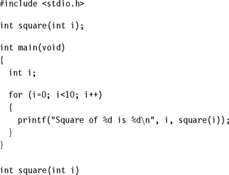
This example shows how to convert a C function to an assembly function—usually the first stage of assembly optimization. Consider the simple C program main.c following that prints the squares of the integers from 0 to 9:
![]()
Let’s see how to replace square by an assembly function that performs the same action. Remove the C definition of square, but not the declaration (the second line) to produce a new C file main1.c. Next add an armasm assembler file square.s with the following contents:
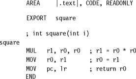
The AREA directive names the area or code section that the code lives in. If you use nonalphanumeric characters in a symbol or area name, then enclose the name in vertical bars. Many nonalphanumeric characters have special meanings otherwise. In the previous code we define a read-only code area called .text.
The EXPORT directive makes the symbol square available for external linking. At line six we define the symbol square as a code label. Note that armasm treats nonindented text as a label definition.
When square is called, the parameter passing is defined by the ATPCS (see Section 5.4). The input argument is passed in register r0, and the return value is returned in register r0. The multiply instruction has a restriction that the destination register must not be the same as the first argument register. Therefore we place the multiply result into r1 and move this to r0.
The END directive marks the end of the assembly file. Comments follow a semicolon. The following script illustrates how to build this example using command line tools.
![]()
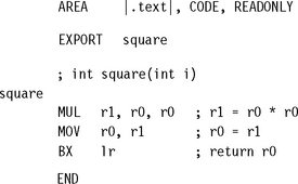
Example 6.1 only works if you are compiling your C as ARM code. If you compile your C as Thumb code, then the assembly routine must return using a BX instruction.
EXAMPLE 6.2
When calling ARM code from C compiled as Thumb, the only change required to the assembly in Example 6.1 is to change the return instruction to a BX. BX will return to ARM or Thumb state according to bit 0 of lr. Therefore this routine can be called from ARM or Thumb. Use BX lr instead of MOV pc, lr whenever your processor supports BX (ARMv4T and above). Create a new assembly file square2.s as follows:
With this example we build the C file using the Thumb C compiler tcc. We assemble the assembly file with the interworking flag enabled so that the linker will allow the Thumb C code to call the ARM assembly code. You can use the following commands to build this example:
![]()
EXAMPLE 6.3
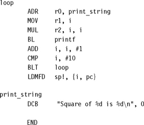
This example shows how to call a subroutine from an assembly routine. We will take Example 6.1 and convert the whole program (including main) into assembly. We will call the C library routine printf as a subroutine. Create a new assembly file main3.s with the following contents:
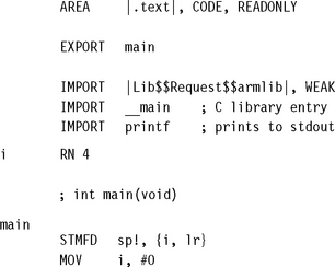
We have used a new directive, IMPORT, to declare symbols that are defined in other files. The imported symbol Lib$$Request$$armlib makes a request that the linker links with the standard ARM C library. The WEAK specifier prevents the linker from giving an error if the symbol is not found at link time. If the symbol is not found, it will take the value zero. The second imported symbol __main is the start of the C library initialization code.
You only need to import these symbols if you are defining your own main; a main defined in C code will import these automatically for you. Importing printf allows us to call that C library function.
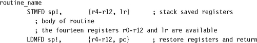
The RN directive allows us to use names for registers. In this case we define i as an alternate name for register r4. Using register names makes the code more readable. It is also easier to change the allocation of variables to registers at a later date.
Recall that ATPCS states that a function must preserve registers r4 to r11 and sp. We corrupt i(r4), and calling printf will corrupt lr. Therefore we stack these two registers at the start of the function using an STMFD instruction. The LDMFD instruction pulls these registers from the stack and returns by writing the return address to pc.
The DCB directive defines byte data described as a string or a comma-separated list of bytes.
To build this example you can use the following command line script:
![]()
Note that Example 6.3 also assumes that the code is called from ARM code. If the code can be called from Thumb code as in Example 6.2 then we must be capable of returning to Thumb code. For architectures before ARMv5 we must use a BX to return. Change the last instruction to the two instructions:
![]()
Finally, let’s look at an example where we pass more than four parameters. Recall that ATPCS places the first four arguments in registers r0 to r3. Subsequent arguments are placed on the stack.
EXAMPLE 6.4
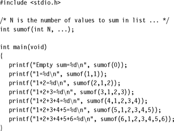
This example defines a function sumof that can sum any number of integers. The arguments are the number of integers to sum followed by a list of the integers. The sumof function is written in assembly and can accept any number of arguments. Put the C part of the example in a file main4.c:
Next define the sumof function in an assembly file sumof.s:

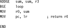
The code keeps count of the number of remaining values to sum, N. The first three values are in registers r1, r2, r3. The remaining values are on the stack. You can build this example using the commands
![]()
6.2 PROFILING AND CYCLE COUNTING
The first stage of any optimization process is to identify the critical routines and measure their current performance. A profiler is a tool that measures the proportion of time or processing cycles spent in each subroutine. You use a profiler to identify the most critical routines. A cycle counter measures the number of cycles taken by a specific routine. You can measure your success by using a cycle counter to benchmark a given subroutine before and after an optimization.
The ARM simulator used by the ADS1.1 debugger is called the ARMulator and provides profiling and cycle counting features. The ARMulator profiler works by sampling the program counter pc at regular intervals. The profiler identifies the function the pc points to and updates a hit counter for each function it encounters. Another approach is to use the trace output of a simulator as a source for analysis.
Be sure that you know how the profiler you are using works and the limits of its accuracy. A pc-sampled profiler can produce meaningless results if it records too few samples. You can even implement your own pc-sampled profiler in a hardware system using timer interrupts to collect the pc data points. Note that the timing interrupts will slow down the system you are trying to measure!
ARM implementations do not normally contain cycle-counting hardware, so to easily measure cycle counts you should use an ARM debugger with ARM simulator. You can configure the ARMulator to simulate a range of different ARM cores and obtain cycle count benchmarks for a number of platforms.
6.3 INSTRUCTION SCHEDULING
The time taken to execute instructions depends on the implementation pipeline. For this chapter, we assume ARM9TDMI pipeline timings. You can find these in Section D.3 of Appendix D. The following rules summarize the cycle timings for common instruction classes on the ARM9TDMI.
Instructions that are conditional on the value of the ARM condition codes in the cpsr take one cycle if the condition is not met. If the condition is met, then the following rules apply:
![]() ALU operations such as addition, subtraction, and logical operations take one cycle. This includes a shift by an immediate value. If you use a register-specified shift, then add one cycle. If the instruction writes to the pc, then add two cycles.
ALU operations such as addition, subtraction, and logical operations take one cycle. This includes a shift by an immediate value. If you use a register-specified shift, then add one cycle. If the instruction writes to the pc, then add two cycles.
![]() Load instructions that load N 32-bit words of memory such as LDR and LDM take N cycles to issue, but the result of the last word loaded is not available on the following cycle. The updated load address is available on the next cycle. This assumes zero-wait-state memory for an uncached system, or a cache hit for a cached system. An LDM of a single value is exceptional, taking two cycles. If the instruction loads pc, then add two cycles.
Load instructions that load N 32-bit words of memory such as LDR and LDM take N cycles to issue, but the result of the last word loaded is not available on the following cycle. The updated load address is available on the next cycle. This assumes zero-wait-state memory for an uncached system, or a cache hit for a cached system. An LDM of a single value is exceptional, taking two cycles. If the instruction loads pc, then add two cycles.
![]() Load instructions that load 16-bit or 8-bit data such as LDRB, LDRSB, LDRH, and LDRSH take one cycle to issue. The load result is not available on the following two cycles. The updated load address is available on the next cycle. This assumes zero-wait-state memory for an uncached system, or a cache hit for a cached system.
Load instructions that load 16-bit or 8-bit data such as LDRB, LDRSB, LDRH, and LDRSH take one cycle to issue. The load result is not available on the following two cycles. The updated load address is available on the next cycle. This assumes zero-wait-state memory for an uncached system, or a cache hit for a cached system.
![]() Branch instructions take three cycles.
Branch instructions take three cycles.
![]() Store instructions that store N values take N cycles. This assumes zero-wait-state memory for an uncached system, or a cache hit or a write buffer with N free entries for a cached system. An STM of a single value is exceptional, taking two cycles.
Store instructions that store N values take N cycles. This assumes zero-wait-state memory for an uncached system, or a cache hit or a write buffer with N free entries for a cached system. An STM of a single value is exceptional, taking two cycles.
![]() Multiply instructions take a varying number of cycles depending on the value of the second operand in the product (see Table D.6 in Section D.3).
Multiply instructions take a varying number of cycles depending on the value of the second operand in the product (see Table D.6 in Section D.3).
To understand how to schedule code efficiently on the ARM, we need to understand the ARM pipeline and dependencies. The ARM9TDMI processor performs five operations in parallel:
![]() Fetch: Fetch from memory the instruction at address pc. The instruction is loaded into the core and then processes down the core pipeline.
Fetch: Fetch from memory the instruction at address pc. The instruction is loaded into the core and then processes down the core pipeline.
![]() Decode: Decode the instruction that was fetched in the previous cycle. The processor also reads the input operands from the register bank if they are not available via one of the forwarding paths.
Decode: Decode the instruction that was fetched in the previous cycle. The processor also reads the input operands from the register bank if they are not available via one of the forwarding paths.
![]() ALU: Executes the instruction that was decoded in the previous cycle. Note this instruction was originally fetched from address pc – 8 (ARM state) or pc – 4 (Thumb state). Normally this involves calculating the answer for a data processing operation, or the address for a load, store, or branch operation. Some instructions may spend several cycles in this stage. For example, multiply and register-controlled shift operations take several ALU cycles.
ALU: Executes the instruction that was decoded in the previous cycle. Note this instruction was originally fetched from address pc – 8 (ARM state) or pc – 4 (Thumb state). Normally this involves calculating the answer for a data processing operation, or the address for a load, store, or branch operation. Some instructions may spend several cycles in this stage. For example, multiply and register-controlled shift operations take several ALU cycles.
![]() LS1: Load or store the data specified by a load or store instruction. If the instruction is not a load or store, then this stage has no effect.
LS1: Load or store the data specified by a load or store instruction. If the instruction is not a load or store, then this stage has no effect.
![]() LS2: Extract and zero- or sign-extend the data loaded by a byte or halfword load instruction. If the instruction is not a load of an 8-bit byte or 16-bit halfword item, then this stage has no effect.
LS2: Extract and zero- or sign-extend the data loaded by a byte or halfword load instruction. If the instruction is not a load of an 8-bit byte or 16-bit halfword item, then this stage has no effect.
Figure 6.1 shows a simplified functional view of the five-stage ARM9TDMI pipeline. Note that multiply and register shift operations are not shown in the figure.
After an instruction has completed the five stages of the pipeline, the core writes the result to the register file. Note that pc points to the address of the instruction being fetched. The ALU is executing the instruction that was originally fetched from address pc – 8 in parallel with fetching the instruction at address pc.
How does the pipeline affect the timing of instructions? Consider the following examples. These examples show how the cycle timings change because an earlier instruction must complete a stage before the current instruction can progress down the pipeline. To work out how many cycles a block of code will take, use the tables in Appendix D that summarize the cycle timings and interlock cycles for a range of ARM cores.
If an instruction requires the result of a previous instruction that is not available, then the processor stalls. This is called a pipeline hazard or pipeline interlock.
EXAMPLE 6.5
This example shows the case where there is no interlock.
![]()
This instruction pair takes two cycles. The ALU calculates r0 + r1 in one cycle. Therefore this result is available for the ALU to calculate r0 + r2 in the second cycle.
EXAMPLE 6.6
This example shows a one-cycle interlock caused by load use.
![]()
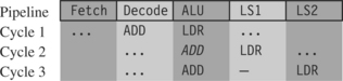
This instruction pair takes three cycles. The ALU calculates the address r2 + 4 in the first cycle while decoding the ADD instruction in parallel. However, the ADD cannot proceed on the second cycle because the load instruction has not yet loaded the value of r1. Therefore the pipeline stalls for one cycle while the load instruction completes the LS1 stage. Now that r1 is ready, the processor executes the ADD in the ALU on the third cycle.
Figure 6.2 illustrates how this interlock affects the pipeline. The processor stalls the ADD instruction for one cycle in the ALU stage of the pipeline while the load instruction completes the LS1 stage. We’ve denoted this stall by an italic ADD. Since the LDR instruction proceeds down the pipeline, but the ADD instruction is stalled, a gap opens up between them. This gap is sometimes called a pipeline bubble. We’ve marked the bubble with a dash.
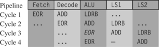
EXAMPLE 6.7
This example shows a one-cycle interlock caused by delayed load use.
![]()
This instruction triplet takes four cycles. Although the ADD proceeds on the cycle following the load byte, the EOR instruction cannot start on the third cycle. The r1 value is not ready until the load instruction completes the LS2 stage of the pipeline. The processor stalls the EOR instruction for one cycle.
Note that the ADD instruction does not affect the timing at all. The sequence takes four cycles whether it is there or not! Figure 6.3 shows how this sequence progresses through the processor pipeline. The ADD doesn’t cause any stalls since the ADD does not use r1, the result of the load.
EXAMPLE 6.8
This example shows why a branch instruction takes three cycles. The processor must flush the pipeline when jumping to a new address.
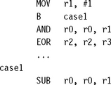
The three executed instructions take a total of five cycles. The MOV instruction executes on the first cycle. On the second cycle, the branch instruction calculates the destination address. This causes the core to flush the pipeline and refill it using this new pc value. The refill takes two cycles. Finally, the SUB instruction executes normally. Figure 6.4 illustrates the pipeline state on each cycle. The pipeline drops the two instructions following the branch when the branch takes place.
6.3.1 SCHEDULING OF LOAD INSTRUCTIONS
Load instructions occur frequently in compiled code, accounting for approximately one-third of all instructions. Careful scheduling of load instructions so that pipeline stalls don’t occur can improve performance. The compiler attempts to schedule the code as best it can, but the aliasing problems of C that we looked at in Section 5.6 limits the available optimizations. The compiler cannot move a load instruction before a store instruction unless it is certain that the two pointers used do not point to the same address.
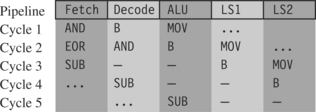
Let’s consider an example of a memory-intensive task. The following function, str_tolower, copies a zero-terminated string of characters from in to out. It converts the string to lowercase in the process.

The ADS1.1 compiler generates the following compiled output. Notice that the compiler optimizes the condition (c>=‘A’ && c<=‘Z’) to the check that 0<=c-‘A’<=‘Z’-‘A’. The compiler can perform this check using a single unsigned comparison.
Unfortunately, the SUB instruction uses the value of c directly after the LDRB instruction that loads c. Consequently, the ARM9TDMI pipeline will stall for two cycles. The compiler can’t do any better since everything following the load of c depends on its value. However, there are two ways you can alter the structure of the algorithm to avoid the cycles by using assembly. We call these methods load scheduling by preloading and unrolling.
6.3.1.1 Load Scheduling by Preloading
In this method of load scheduling, we load the data required for the loop at the end of the previous loop, rather than at the beginning of the current loop. To get performance improvement with little increase in code size, we don’t unroll the loop.
EXAMPLE 6.9
This assembly applies the preload method to the str_tolower function.
![]()
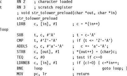
The scheduled version is one instruction longer than the C version, but we save two cycles for each inner loop iteration. This reduces the loop from 11 cycles per character to 9 cycles per character on an ARM9TDMI, giving a 1.22 times speed improvement.
The ARM architecture is particularly well suited to this type of preloading because instructions can be executed conditionally. Since loop i is loading the data for loop i +1 there is always a problem with the first and last loops. For the first loop, we can preload data by inserting extra load instructions before the loop starts. For the last loop it is essential that the loop does not read any data, or it will read beyond the end of the array. This could cause a data abort! With ARM, we can easily solve this problem by making the load instruction conditional. In Example 6.9, the preload of the next character only takes place if the loop will iterate once more. No byte load occurs on the last loop.
6.3.1.2 Load Scheduling by Unrolling
This method of load scheduling works by unrolling and then interleaving the body of the loop. For example, we can perform loop iterations i, i +1, i + 2 interleaved. When the result of an operation from loop i is not ready, we can perform an operation from loop i + 1 that avoids waiting for the loop i result.
EXAMPLE 6.10
The assembly applies load scheduling by unrolling to the str_tolower function.
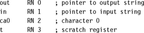
This loop is the most efficient implementation we’ve looked at so far. The implementation requires seven cycles per character on ARM9TDMI. This gives a 1.57 times speed increase over the original str_tolower. Again it is the conditional nature of the ARM instructions that makes this possible. We use conditional instructions to avoid storing characters that are past the end of the string.
However, the improvement in Example 6.10 does have some costs. The routine is more than double the code size of the original implementation. We have assumed that you can read up to two characters beyond the end of the input string, which may not be true if the string is right at the end of available RAM, where reading off the end will cause a data abort. Also, performance can be slower for very short strings because (1) stacking lr causes additional function call overhead and (2) the routine may process up to two characters pointlessly, before discovering that they lie beyond the end of the string.
You should use this form of scheduling by unrolling for time-critical parts of an application where you know the data size is large. If you also know the size of the data at compile time, you can remove the problem of reading beyond the end of the array.
SUMMARY: Instruction Scheduling
![]() ARM cores have a pipeline architecture. The pipeline may delay the results of certain instructions for several cycles. If you use these results as source operands in a following instruction, the processor will insert stall cycles until the value is ready.
ARM cores have a pipeline architecture. The pipeline may delay the results of certain instructions for several cycles. If you use these results as source operands in a following instruction, the processor will insert stall cycles until the value is ready.
![]() Load and multiply instructions have delayed results in many implementations. See Appendix D for the cycle timings and delay for your specific ARM processor core.
Load and multiply instructions have delayed results in many implementations. See Appendix D for the cycle timings and delay for your specific ARM processor core.
![]() You have two software methods available to remove interlocks following load instructions: You can preload so that loop i loads the data for loop i + 1, or you can unroll the loop and interleave the code for loops i and i +1.
You have two software methods available to remove interlocks following load instructions: You can preload so that loop i loads the data for loop i + 1, or you can unroll the loop and interleave the code for loops i and i +1.
6.4 REGISTER ALLOCATION
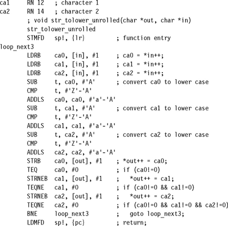
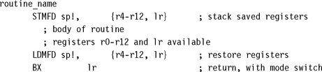
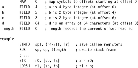
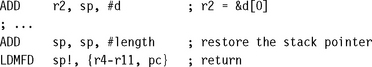
You can use 14 of the 16 visible ARM registers to hold general-purpose data. The other two registers are the stack pointer r13 and the program counter r15. For a function to be ATPCS compliant it must preserve the callee values of registers r4 to r11. ATPCS also specifies that the stack should be eight-byte aligned; therefore you must preserve this alignment if calling subroutines. Use the following template for optimized assembly routines requiring many registers:
Our only purpose in stacking r12 is to keep the stack eight-byte aligned. You need not stack r12 if your routine doesn’t call other ATPCS routines. For ARMv5 and above you can use the preceding template even when being called from Thumb code. If your routine may be called from Thumb code on an ARMv4T processor, then modify the template as follows:
In this section we look at how best to allocate variables to register numbers for registerintensive tasks, how to use more than 14 local variables, and how to make the best use of the 14 available registers.
6.4.1 ALLOCATING VARIABLES TO REGISTER NUMBERS
When you write an assembly routine, it is best to start by using names for the variables, rather than explicit register numbers. This allows you to change the allocation of variables to register numbers easily. You can even use different register names for the same physical register number when their use doesn’t overlap. Register names increase the clarity and readability of optimized code.
For the most part ARM operations are orthogonal with respect to register number. In other words, specific register numbers do not have specific roles. If you swap all occurrences of two registers Ra and Rb in a routine, the function of the routine does not change. However, there are several cases where the physical number of the register is important:
![]() Argument registers. The ATPCS convention defines that the first four arguments to a function are placed in registers r0 to r3. Further arguments are placed on the stack. The return value must be placed in r0.
Argument registers. The ATPCS convention defines that the first four arguments to a function are placed in registers r0 to r3. Further arguments are placed on the stack. The return value must be placed in r0.
![]() Registers used in a load or store multiple. Load and store multiple instructions LDM and STM operate on a list of registers in order of ascending register number. If r0 and r1 appear in the register list, then the processor will always load or store r0 using a lower address than r1 and so on.
Registers used in a load or store multiple. Load and store multiple instructions LDM and STM operate on a list of registers in order of ascending register number. If r0 and r1 appear in the register list, then the processor will always load or store r0 using a lower address than r1 and so on.
![]() Load and store double word. The LDRD and STRD instructions introduced in ARMv5E operate on a pair of registers with sequential register numbers, Rd and Rd +1. Furthermore, Rd must be an even register number.
Load and store double word. The LDRD and STRD instructions introduced in ARMv5E operate on a pair of registers with sequential register numbers, Rd and Rd +1. Furthermore, Rd must be an even register number.
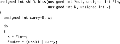
For an example of how to allocate registers when writing assembly, suppose we want to shift an array of N bits upwards in memory by k bits. For simplicity assume that N is large and a multiple of 256. Also assume that 0 ≤ k < 32 and that the input and output pointers are word aligned. This type of operation is common in dealing with the arithmetic of multiple precision numbers where we want to multiply by 2k. It is also useful to block copy from one bit or byte alignment to a different bit or byte alignment. For example, the C library function memcpy can use the routine to copy an array of bytes using only word accesses.
The C routine shift_bits implements the simple k-bit shift of N bits of data. It returns the k bits remaining following the shift.
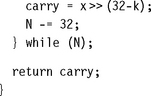
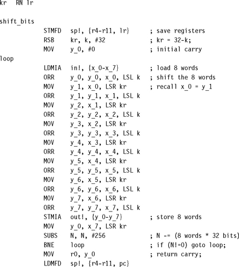
The obvious way to improve efficiency is to unroll the loop to process eight words of 256 bits at a time so that we can use load and store multiple operations to load and store eight words at a time for maximum efficiency. Before thinking about register numbers, we write the following assembly code:
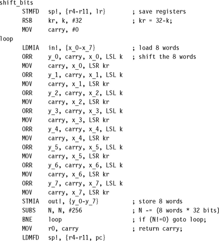
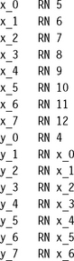
Now to the register allocation. So that the input arguments do not have to move registers, we can immediately assign
![]()
![]()
For the load multiple to work correctly, we must assign x0 through x7 to sequentially increasing register numbers, and similarly for y0 through y7. Notice that we finish with x0 before starting with y1. In general, we can assign xn to the same register as yn+1. Therefore, assign
We are nearly finished, but there is a problem. There are two remaining variables carry and kr, but only one remaining free register lr. There are several possible ways we can proceed when we run out of registers:
![]() Reduce the number of registers we require by performing fewer operations in each loop. In this case we could load four words in each load multiple rather than eight.
Reduce the number of registers we require by performing fewer operations in each loop. In this case we could load four words in each load multiple rather than eight.
![]() Use the stack to store the least-used values to free up more registers. In this case we could store the loop counter N on the stack. (See Section 6.4.2 for more details on swapping registers to the stack.)
Use the stack to store the least-used values to free up more registers. In this case we could store the loop counter N on the stack. (See Section 6.4.2 for more details on swapping registers to the stack.)
![]() Alter the code implementation to free up more registers. This is the solution we consider in the following text. (For more examples, see Section 6.4.3.)
Alter the code implementation to free up more registers. This is the solution we consider in the following text. (For more examples, see Section 6.4.3.)
We often iterate the process of implementation followed by register allocation several times until the algorithm fits into the 14 available registers. In this case we notice that the carry value need not stay in the same register at all! We can start off with the carry value in y0 and then move it to y1 when x0 is no longer required, and so on. We complete the routine by allocating kr to lr and recoding so that carry is not required.
6.4.2 USING MORE THAN 14 LOCAL VARIABLES
If you need more than 14 local 32-bit variables in a routine, then you must store some variables on the stack. The standard procedure is to work outwards from the innermost loop of the algorithm, since the innermost loop has the greatest performance impact.
EXAMPLE 6.12
This example shows three nested loops, each loop requiring state information inherited from the loop surrounding it. (See Section 6.6 for further ideas and examples of looping constructs.)
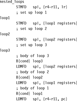
You may find that there are insufficient registers for the innermost loop even using the construction in Example 6.12. Then you need to swap inner loop variables out to the stack. Since assembly code is very hard to maintain and debug if you use numbers as stack address offsets, the assembler provides an automated procedure for allocating variables to the stack.
6.4.3 MAKING THE MOST OF AVAILABLE REGISTERS
On a load-store architecture such as the ARM, it is more efficient to access values held in registers than values held in memory. There are several tricks you can use to fit several sub-32-bit length variables into a single 32-bit register and thus can reduce code size and increase performance. This section presents three examples showing how you can pack multiple variables into a single ARM register.
EXAMPLE 6.14
Suppose we want to step through an array by a programmable increment. A common example is to step through a sound sample at various rates to produce different pitched notes. We can express this in C code as
![]()
Commonly index and increment are small enough to be held as 16-bit values. We can pack these two variables into a single 32-bit variable indinc:
![]()
The C code translates into assembly code using a single register to hold indinc:
![]()
Note that if index and increment are 16-bit values, then putting index in the top 16 bits of indinc correctly implements 16-bit-wrap-around. In other words, index = (short)(index + increment). This can be useful if you are using a buffer where you want to wrap from the end back to the beginning (often known as a circular buffer).
EXAMPLE 6.15
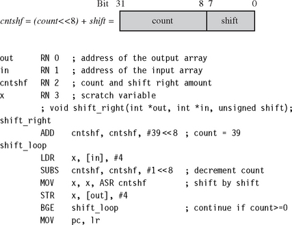
When you shift by a register amount, the ARM uses bits 0 to 7 as the shift amount. The ARM ignores bits 8 to 31 of the register. Therefore you can use bits 8 to 31 to hold a second variable distinct from the shift amount.
This example shows how to combine a register-specified shift shift and loop counter count to shift an array of 40 entries right by shift bits. We define a new variable cntshf that combines count and shift:
EXAMPLE 6.16
If you are dealing with arrays of 8-bit or 16-bit values, it is sometimes possible to manipulate multiple values at a time by packing several values into a single 32-bit register. This is called single issue multiple data (SIMD) processing.
ARM architecture versions up to ARMv5 do not support SIMD operations explicitly. However, there are still areas where you can achieve SIMD type compactness. Section 6.6 shows how you can store multiple loop values in a single register. Here we look at a graphics example of how to process multiple 8-bit pixels in an image using normal ADD and MUL instructions to achieve some SIMD operations.
Suppose we want to merge two images X and Y to produce a new image Z. Let xn, yn, and zn denote the nth 8-bit pixel in these images, respectively. Let 0 ≤ a ≤ 256 be a scaling factor. To merge the images, we set
In other words image Z is image X scaled in intensity by a/256 added to image Y scaled by 1 – (a/256). Note that
Therefore each pixel requires a subtract, a multiply, a shifted add, and a right shift. To process multiple pixels at a time, we load four pixels at once using a word load. We use a bracketed notation to denote several values packed into the same word:
![]()
We then unpack the 8-bit data and promote it to 16-bit data using an AND with a mask register. We use the notation
![]()
Note that even for signed values [a, b] + [c, d] = [a + b, c + d] if we interpret [a, b] using the mathematical equation a216 + b. Therefore we can perform SIMD operations on these values using normal arithmetic instructions.
The following code shows how you can process four pixels at a time using only two multiplies. The code assumes a 176 144 sized quarter CIF image.
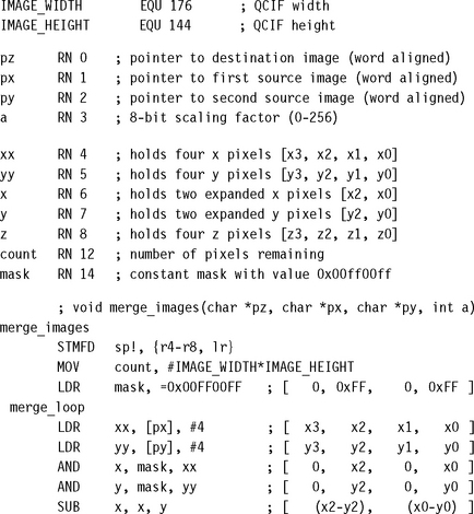
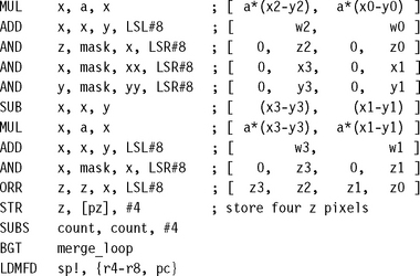
Therefore it is easy to separate the value [w2, w0] into w2 and w0 by taking the most significant and least significant 16-bit portions, respectively. We have succeeded in processing four 8-bit pixels using 32-bit load, stores, and data operations to perform operations in parallel.
![]() ARM has 14 available registers for general-purpose use: r0 to r12 and r14. The stack pointer r13 and program counter r15 cannot be used for general-purpose data. Operating system interrupts often assume that the user mode r13 points to a valid stack, so don’t be tempted to reuse r13.
ARM has 14 available registers for general-purpose use: r0 to r12 and r14. The stack pointer r13 and program counter r15 cannot be used for general-purpose data. Operating system interrupts often assume that the user mode r13 points to a valid stack, so don’t be tempted to reuse r13.
![]() If you need more than 14 local variables, swap the variables out to the stack, working outwards from the innermost loop.
If you need more than 14 local variables, swap the variables out to the stack, working outwards from the innermost loop.
![]() Use register names rather than physical register numbers when writing assembly routines. This makes it easier to reallocate registers and to maintain the code.
Use register names rather than physical register numbers when writing assembly routines. This makes it easier to reallocate registers and to maintain the code.
![]() To ease register pressure you can sometimes store multiple values in the same register. For example, you can store a loop counter and a shift in one register. You can also store multiple pixels in one register.
To ease register pressure you can sometimes store multiple values in the same register. For example, you can store a loop counter and a shift in one register. You can also store multiple pixels in one register.
6.5 CONDITIONAL EXECUTION
The processor core can conditionally execute most ARM instructions. This conditional execution is based on one of 15 condition codes. If you don’t specify a condition, the assembler defaults to the execute always condition (AL). The other 14 conditions split into seven pairs of complements. The conditions depend on the four condition code flags N, Z, C, V stored in the cpsr register. See Table A.2 in Appendix A for the list of possible ARM conditions. Also see Sections 2.2.6 and 3.8 for an introduction to conditional execution.
By default, ARM instructions do not update the N, Z, C, V flags in the ARM cpsr. For most instructions, to update these flags you append an S suffix to the instruction mnemonic. Exceptions to this are comparison instructions that do not write to a destination register. Their sole purpose is to update the flags and so they don’t require the S suffix.
By combining conditional execution and conditional setting of the flags, you can implement simple if statements without any need for branches. This improves efficiency since branches can take many cycles and also reduces code size.
EXAMPLE 6.17
The following C code converts an unsigned integer 0 ≤ i ≤ 15 to a hexadecimal character c:
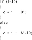
We can write this in assembly using conditional execution rather than conditional branches:
![]()
The sequence works since the first ADD does not change the condition codes. The second ADD is still conditional on the result of the compare. Section 6.3.1 shows a similar use of conditional execution to convert to lowercase.
Conditional execution is even more powerful for cascading conditions.
EXAMPLE 6.18
The following C code identifies if c is a vowel:
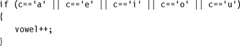
In assembly you can write this using conditional comparisons:
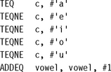
As soon as one of the TEQ comparisons detects a match, the Z flag is set in the cpsr. The following TEQNE instructions have no effect as they are conditional on Z = 0.
The next instruction to have effect is the ADDEQ that increments vowel. You can use this method whenever all the comparisons in the if statement are of the same type.
EXAMPLE 6.19
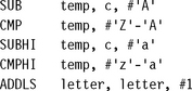
Consider the following code that detects if c is a letter:

To implement this efficiently, we can use an addition or subtraction to move each range to the form 0 ≤ c ≤ limit. Then we use unsigned comparisons to detect this range and conditional comparisons to chain together ranges. The following assembly implements this efficiently:
For more complicated decisions involving switches, see Section 6.8.
Note that the logical operations AND and OR are related by the standard logical relations as shown in Table 6.1. You can invert logical expressions involving OR to get an expression involving AND, which can often be useful in simplifying or rearranging logical expressions.
Table 6.1
| Inverted expression | Equivalent |
| !(a && b) | (!a) || (!b) |
| !(a || b) | (!a) && (!b) |
SUMMARY: Conditional Execution
![]() You can implement most if statements with conditional execution. This is more efficient than using a conditional branch.
You can implement most if statements with conditional execution. This is more efficient than using a conditional branch.
![]() You can implement if statements with the logical AND or OR of several similar conditions using compare instructions that are themselves conditional.
You can implement if statements with the logical AND or OR of several similar conditions using compare instructions that are themselves conditional.
6.6 LOOPING CONSTRUCTS
Most routines critical to performance will contain a loop. We saw in Section 5.3 that on the ARM loops are fastest when they count down towards zero. This section describes how to implement these loops efficiently in assembly. We also look at examples of how to unroll loops for maximum performance.
6.6.1 DECREMENTED COUNTED LOOPS
For a decrementing loop of N iterations, the loop counter i counts down from N to 1 inclusive. The loop terminates with i = 0. An efficient implementation is
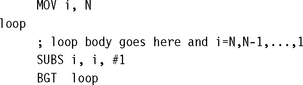
The loop overhead consists of a subtraction setting the condition codes followed by a conditional branch. On ARM7 and ARM9 this overhead costs four cycles per loop. If i is an array index, then you may want to count down from N – 1 to 0 inclusive instead so that you can access array element zero. You can implement this in the same way by using a different conditional branch:

In this arrangement the Z flag is set on the last iteration of the loop and cleared for other iterations. If there is anything different about the last loop, then we can achieve this using the EQ and NE conditions. For example, if you preload data for the next loop (as discussed in Section 6.3.1.1), then you want to avoid the preload on the last loop. You can make all preload operations conditional on NE as in Section 6.3.1.1.
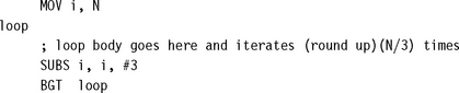
There is no reason why we must decrement by one on each loop. Suppose we require N/3 loops. Rather than attempting to divide N by three, it is far more efficient to subtract three from the loop counter on each iteration:
6.6.2 UNROLLED COUNTED LOOPS
This brings us to the subject of loop unrolling. Loop unrolling reduces the loop overhead by executing the loop body multiple times. However, there are problems to overcome. What if the loop count is not a multiple of the unroll amount? What if the loop count is smaller than the unroll amount? We looked at these questions for C code in Section 5.3. In this section we look at how you can handle these issues in assembly.
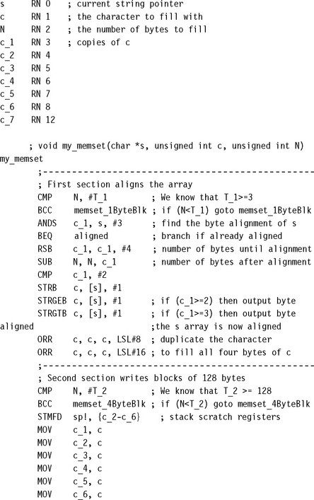
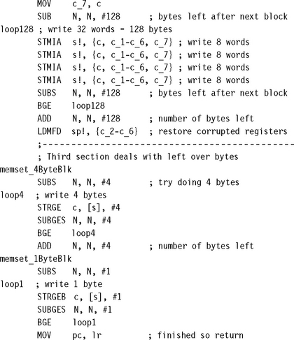
We’ll take the C library function memset as a case study. This function sets N bytes of memory at address s to the byte value c. The function needs to be efficient, so we will look at how to unroll the loop without placing extra restrictions on the input operands. Our version of memset will have the following C prototype:
![]()
To be efficient for large N, we need to write multiple bytes at a time using STR or STM instructions. Therefore our first task is to align the array pointer s. However, it is only worth us doing this if N is sufficiently large. We aren’t sure yet what “sufficiently large” means, but let’s assume we can choose a threshold value T1 and only bother to align the array when N ≥ T1. Clearly T1 ≥ 3 as there is no point in aligning if we don’t have four bytes to write!
Now suppose we have aligned the array s. We can use store multiples to set memory efficiently. For example, we can use a loop of four store multiples of eight words each to set 128 bytes on each loop. However, it will only be worth doing this if N ≥ T2 ≥ 128, where T2 is another threshold to be determined later on.
Finally, we are left with N < T2 bytes to set. We can write bytes in blocks of four using STR until N < 4. Then we can finish by writing bytes singly with STRB to the end of the array.
EXAMPLE 6.20
This example shows the unrolled memset routine. We’ve separated the three sections corresponding to the preceding paragraphs with rows of dashes. The routine isn’t finished until we’ve decided the best values for T1 and T2.
It remains to find the best values for the thresholds T1 and T2. To determine these we need to analyze the cycle counts for different ranges of N. Since the algorithm operates on blocks of size 128 bytes, 4 bytes, and 1 byte, respectively, we start by decomposing N with respect to these block sizes:
We now partition into three cases. To follow the details of these cycle counts, you will need to refer to the instruction cycle timings in Appendix D.
![]() Case 0 ≤ N < T1: The routine takes 5N + 6 cycles on an ARM9TDMI including the return.
Case 0 ≤ N < T1: The routine takes 5N + 6 cycles on an ARM9TDMI including the return.
![]() Case T1 ≤ N < T2: The first algorithm block takes 6 cycles if the s array is word aligned and 10 cycles otherwise. Assuming each alignment is equally likely, this averages to (6 + 10 + 10 + 10)/4 = 9 cycles. The second algorithm block takes 6 cycles. The final block takes 5(32Nh + Nm) + 5(Nl + Zl) + 2 cycles, where Zl is 1 if Nl = 0, and 0 otherwise. The total cycles for this case is 5(32Nh + Nm + Nl + Zl) + 17.
Case T1 ≤ N < T2: The first algorithm block takes 6 cycles if the s array is word aligned and 10 cycles otherwise. Assuming each alignment is equally likely, this averages to (6 + 10 + 10 + 10)/4 = 9 cycles. The second algorithm block takes 6 cycles. The final block takes 5(32Nh + Nm) + 5(Nl + Zl) + 2 cycles, where Zl is 1 if Nl = 0, and 0 otherwise. The total cycles for this case is 5(32Nh + Nm + Nl + Zl) + 17.
![]() Case N ≥ T2: As in the previous case, the first algorithm block averages 9 cycles. The second algorithm block takes 36Nh + 21 cycles. The final algorithm block takes 5(Nm + Zm + Nl + Zl) + 2 cycles, where Zm is 1 if Nm is 0, and 0 otherwise. The total cycles for this case is 36Nh + 5(Nm + Zm + Nl + Zl) + 32.
Case N ≥ T2: As in the previous case, the first algorithm block averages 9 cycles. The second algorithm block takes 36Nh + 21 cycles. The final algorithm block takes 5(Nm + Zm + Nl + Zl) + 2 cycles, where Zm is 1 if Nm is 0, and 0 otherwise. The total cycles for this case is 36Nh + 5(Nm + Zm + Nl + Zl) + 32.
Table 6.2 summarizes these results. Comparing the three table rows it is clear that the second row wins over the first row as soon as Nm ≥ 1, unless Nm = 1 and Nl = 0. We set T1 = 5 to choose the best cycle counts from rows one and two. The third row wins over the second row as soon as Nh ≥ 1. Therefore take T2 = 128.
Table 6.2
Cycles taken for each range of N values.
| N range | Cycles taken |
| 0 ≤ N < T1 | 640Nh + 20Nm + 5Nl + 6 |
| T1 ≤ N < T2 | 160Nh + 5Nm + 5Nl + 17 + 5Zl |
| T2 ≤ N | 36Nh + 5Nm + 5Nl + 32 + 5Zl + 5Zm |
This detailed example shows you how to unroll any important loop using threshold values and provide good performance over a range of possible input values.
6.6.3 MULTIPLE NESTED LOOPS
How many loop counters does it take to maintain multiple nested loops? Actually, one will suffice—or more accurately, one provided the sum of the bits needed for each loop count does not exceed 32. We can combine the loop counts within a single register, placing the innermost loop count at the highest bit positions. This section gives an example showing how to do this. We will ensure the loops count down from max – 1 to 0 inclusive so that the loop terminates by producing a negative result.
EXAMPLE 6.21
This example shows how to merge three loop counts into a single loop count. Suppose we wish to multiply matrix B by matrix C to produce matrix A, where A, B, C have the following constant dimensions. We assume that R, S, T are relatively large but less than 256.
![]()
We represent each matrix by a lowercase pointer of the same name, pointing to an array of words organized by row. For example, the element at row i, column j, A[i, j], is at the byte address
![]()
A simple C implementation of the matrix multiply uses three nested loops i, j, and k:
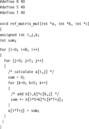
There are many ways to improve the efficiency here, starting by removing the address indexing calculations, but we will concentrate on the looping structure. We allocate a register counter count containing all three loop counters i, j, k:
![]()
Note that S – 1 – k counts from S – 1 down to 0 rather than counting from 0 to S – 1 as k does. The following assembly implements the matrix multiply using this single counter in register count:
![]()

The preceding structure saves two registers over a naive implementation. First, we decrement the count at bits 16 to 23 until the result is negative. This implements the k loop, counting down from S – 1 to 0 inclusive. Once the result is negative, the code adds 216 to clear bits 16 to 31. Then we subtract 28 to decrement the count stored at bits 8 to 15, implementing the j loop. We can encode the constant 216 – 28 = 0xFF00 efficiently using a single ARM instruction. Bits 8 to 15 now count down from T – 1 to 0. When the result of the combined ADD and subtract is negative, then we have finished the j loop. We repeat the same process for the i loop. ARM’s ability to handle a wide range of rotated constants in addition and subtraction instructions makes this scheme very efficient.
6.6.4 OTHER COUNTED LOOPS
You may want to use the value of a loop counter as an input to calculations in the loop. It’s not always desirable to count down from N to 1 or N – 1 to 0. For example, you may want to select bits out of a data register one at a time; in this case you may want a power-of-two mask that doubles on each iteration.
The following subsections show useful looping structures that count in different patterns. They use only a single instruction combined with a branch to implement the loop.
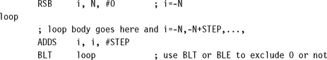
6.6.4.1 Negative Indexing
This loop structure counts from –N to 0 (inclusive or exclusive) in steps of size STEP.
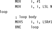
6.6.4.2 Logarithmic Indexing
This loop structure counts down from 2N to 1 in powers of two. For example, if N = 4, then it counts 16, 8, 4, 2, 1.
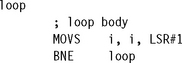
The following loop structure counts down from an N-bit mask to a one-bit mask. For example, if N = 4, then it counts 15, 7, 3, 1.
![]()
![]() ARM requires two instructions to implement a counted loop: a subtract that sets flags and a conditional branch.
ARM requires two instructions to implement a counted loop: a subtract that sets flags and a conditional branch.
![]() Unroll loops to improve loop performance. Do not overunroll because this will hurt cache performance. Unrolled loops may be inefficient for a small number of iterations. You can test for this case and only call the unrolled loop if the number of iterations is large.
Unroll loops to improve loop performance. Do not overunroll because this will hurt cache performance. Unrolled loops may be inefficient for a small number of iterations. You can test for this case and only call the unrolled loop if the number of iterations is large.
![]() Nested loops only require a single loop counter register, which can improve efficiency by freeing up registers for other uses.
Nested loops only require a single loop counter register, which can improve efficiency by freeing up registers for other uses.
![]() ARM can implement negative and logarithmic indexed loops efficiently.
ARM can implement negative and logarithmic indexed loops efficiently.
6.7 BIT MANIPULATION
Compressed file formats pack items at a bit granularity to maximize the data density. The items may be of a fixed width, such as a length FIELD or version field, or they may be of a variable width, such as a Huffman coded symbol. Huffman codes are used in compression to associate with each symbol a code of bits. The code is shorter for common symbols and longer for rarer symbols.
In this section we look at methods to handle a bitstream efficiently. First we look at fixed-width codes, then variable width codes. See Section 7.6 for common bit manipulation routines such as endianness and bit reversal.
6.7.1 FIXED-WIDTH BIT-FIELD PACKING AND UNPACKING
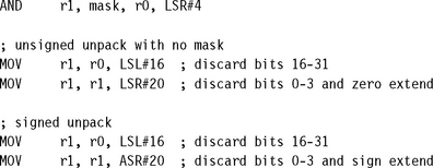
You can extract an unsigned bit-field from an arbitrary position in an ARM register in one cycle provided that you set up a mask in advance; otherwise you require two cycles. A signed bit-field always requires two cycles to unpack unless the bit-field lies at the top of a word (most significant bit of the bit-field is the most significant bit of the register). On the ARM we use logical operations and the barrel shifter to pack and unpack codes, as in the following examples.
6.7.2 VARIABLE-WIDTH BITSTREAM PACKING
Our task here is to pack a series of variable-length codes to create a bitstream. Typically we are compressing a datastream and the variable-length codes represent Huffman or arithmetic coding symbols. However, we don t need to make any assumptions about what the codes represent to pack them efficiently.
We do need to be careful about the packing endianness. Many compressed file formats use a big-endian bit-packing order where the first code is placed at the most significant bits of the first byte. For this reason we will use a big-endian bit-packing order for our examples. This is sometimes known as network order. Figure 6.5 shows how we form a bytestream out of variable-length bitcodes using a big-endian packing order. High and low represent the most and least significant bit ends of the byte.

To implement packing efficiently on the ARM we use a 32-bit register as a buffer to hold four bytes, in big-endian order. In other words we place byte 0 of the bytestream in the most significant 8 bits of the register. Then we can insert codes into the register one at a time, starting from the most significant bit and working down to the least significant bit.
Once the register is full we can store 32 bits to memory. For a big-endian memory system we can store the word without modification. For a little-endian memory system we need to reverse the byte order in the word before storing.
We call the 32-bit register we insert codes into bitbuffer. We need a second register bitsfree to record the number of bits that we haven’t used in bitbuffer. In other words, bitbuffer contains 32 – bitsfree code bits, and bitsfree zero bits, as in Figure 6.6. To insert a code of k bits into bitbuffer, we subtract k from bitsfree and then insert the code with a left shift of bitsfree.
We also need to be careful about alignment. A bytestream need not be word aligned, and so we can’t use word accesses to write it. To allow word accesses we will start by backing up to the last word-aligned address. Then we fill the 32-bit register bitbuffer with the backed-up data. From then on we can use word (32-bit) read and writes.
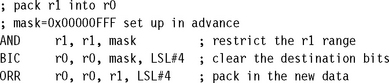
EXAMPLE 6.24
This example provides three functions bitstream_write_start, bitstream_write_code, and bitstream_write_flush. These are not ATPCS-compliant functions because they assume registers such as bitbuffer are preserved between calls. In practice you will inline this code for efficiency, and so this is not a problem.
The bitstream_write_start function aligns the bitstream pointer bitstream and initializes the 32-bit buffer bitbuffer. Each call to bitstream_write_code inserts a value code of bit-length codebits. Finally, the bitstream_write_flush function writes any remaining bytes to the bitstream to terminate the stream.
![]()
6.7.3 VARIABLE-WIDTH BITSTREAM UNPACKING
It is much harder to unpack a bitstream of variable-width codes than to pack it. The problem is that we usually don’t know the width of the codes we are unpacking! For Huffman-encoded bitstreams you must derive the length of each code by looking at the next sequence of bits and working out which code it can be.
Here we will use a lookup table to speed up the unpacking process. The idea is to take the next N bits of the bitstream and perform a lookup in two tables, look_codebits[] and look_code[], each of size 2N entries. If the next N bits are sufficient to determine the code, then the tables tell us the code length and the code value, respectively. If the next N bits are insufficient to determine the code, then the look_codebits table will return an escape value of OxFF. An escape value is just a flag to indicate that this case is exceptional.
In a sequence of Huffman codes, common codes are short and rare codes are long. So, we expect to decode most common codes quickly, using the lookup tables. In the following example we assume that N = 8 and use 256-entry lookup tables.
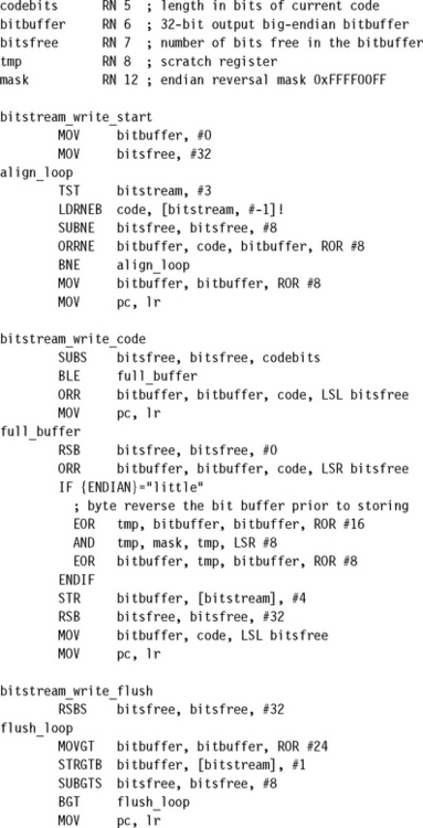
EXAMPLE 6.25
This example provides three functions to unpack a big-endian bitstream stored in a bytestream. As with Example 6.24, these functions are not ATPCS compliant and will normally be inlined. The function bitstream_read_start initializes the process, starting to decode a bitstream at byte address bitstream. Each call to bitstream_read_code returns the next code in register code. The function only handles short codes that can be read from the lookup table. Long codes are trapped at the label long_code, but the implementation of this function depends on the codes you are decoding.
The code uses a register bitbuffer that contains N + bitsleft code bits starting at the most significant bit (see Figure 6.7).

The counter bitsleft actually counts the number of bits remaining in the buffer bitbuffer less the N bits required for the next lookup. Therefore we can perform the next table lookup as long as bitsleft ≥ 0. As soon as bitsleft < 0 there are two possibilities. One possibility is that we found a valid code but then have insufficient bits to look up the next code. Alternatively, codebits contains the escape value 0xFF to indicate that the code was longer than N bits. We can trap both these cases at once using a call to empty_buffer_or_long_code. If the buffer is empty, then we fill it with 24 bits. If we have detected a long code, then we branch to the long_code trap.
The example has a best-case performance of seven cycles per code unpack on an ARM9TDMI. You can obtain faster results if you know the sizes of the packed bitfields in advance.
![]() The ARM can pack and unpack bits efficiently using logical operations and the barrel shifter.
The ARM can pack and unpack bits efficiently using logical operations and the barrel shifter.
![]() To access bitstreams efficiently use a 32-bit register as a bitbuffer. Use a second register to keep track of the number of valid bits in the bitbuffer.
To access bitstreams efficiently use a 32-bit register as a bitbuffer. Use a second register to keep track of the number of valid bits in the bitbuffer.
![]() To decode bitstreams efficiently, use a lookup table to scan the next N bits of the bitstream. The lookup table can return codes of length at most N bits directly, or return an escape character for longer codes.
To decode bitstreams efficiently, use a lookup table to scan the next N bits of the bitstream. The lookup table can return codes of length at most N bits directly, or return an escape character for longer codes.
6.8 EFFICIENT SWITCHES
A switch or multiway branch selects between a number of different actions. In this section we assume the action depends on a variable x. For different values of x we need to perform different actions. This section looks at assembly to implement a switch efficiently for different types of x.
6.8.1 SWITCHES ON THE RANGE 0 ≤ x  N
N
The example C function ref_switch performs different actions according to the value of x. We are only interested in x values in the range 0 ≤ x < 8.

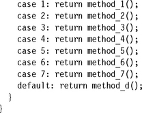
There are two ways to implement this structure efficiently in ARM assembly. The first method uses a table of function addresses. We load pc from the table indexed by x.
EXAMPLE 6.26
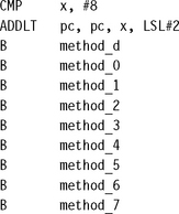
The switch_absolute code performs a switch using an inlined table of function pointers:

The code works because the pc register is pipelined. The pc points to the method_0 word when the ARM executes the LDR instruction.
The method above is very fast, but has one drawback: The code is not position independent since it stores absolute addresses to the method functions in memory. Position-independent code is often used in modules that are installed into a system at run time. The next example shows how to solve this problem.
EXAMPLE 6.27
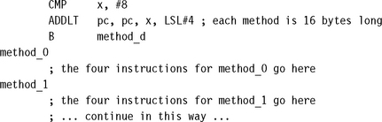
The code switch_relative is slightly slower compared to switch_absolute, but it is position independent:
![]()
There is one final optimization you can make. If the method functions are short, then you can inline the instructions in place of the branch instructions.
6.8.2 SWITCHES ON A GENERAL VALUE
Now suppose that x does not lie in some convenient range 0 ≤ x<N for N small enough to apply the methods of Section 6.8.1. How do we perform the switch efficiently, without having to test x against each possible value in turn?
A very useful technique in these situations is to use a hashing function. A hashing function is any function y = f(x) that maps the values we are interested in into a continuous range of the form 0 ≤ y < N. Instead of a switch on x, we can use a switch on y = f(x). There is a problem if we have a collision, that is, if two x values MAP to the same y value. In this case we need further code to test all the possible x values that could have led to the y value. For our purposes a good hashing function is easy to compute and does not suffer from many collisions.
To perform the switch we apply the hashing function and then use the optimized switch code of Section 6.8.1 on the hash value y. Where two x values can MAP to the same hash, we need to perform an explicit test, but this should be rare for a good hash function.
EXAMPLE 6.29
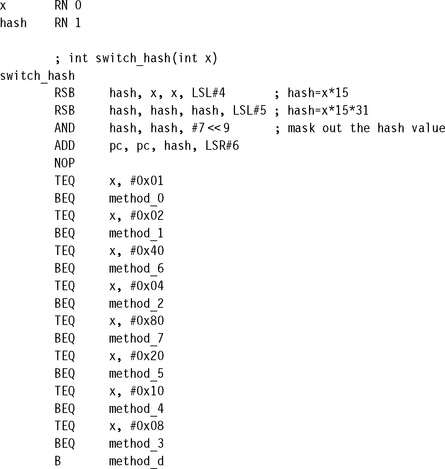
Suppose we want to call method_k when x = 2k for eight possible methods. In other words we want to switch on the values 1, 2, 4, 8, 16, 32, 64, 128. For all other values of x we need to call the default method method_d. We look for a hash function formed out of multiplying by powers of two minus one (this is an efficient operation on the ARM). By trying different multipliers we find that 15 × 31 × x has a different value in bits 9 to 11 for each of the eight switch values. This means we can use bits 9 to 11 of this product as our hash function.
The following switch_hash assembly uses this hash function to perform the switch. Note that other values that are not powers of two will have the same hashes as the values we want to detect. The switch has narrowed the case down to a single power of two that we can test for explicitly. If x is not a power of two, then we fall through to the default case of calling method_d.
![]() Make sure the switch value is in the range 0 ≤ x < N for some small N. To do this you may have to use a hashing function.
Make sure the switch value is in the range 0 ≤ x < N for some small N. To do this you may have to use a hashing function.
![]() Use the switch value to index a table of function pointers or to branch to short sections of code at regular intervals. The second technique is position independent; the first isn’t.
Use the switch value to index a table of function pointers or to branch to short sections of code at regular intervals. The second technique is position independent; the first isn’t.
6.9 HANDLING UNALIGNED DATA
Recall that a load or store is unaligned if it uses an address that is not a multiple of the data transfer width. For code to be portable across ARM architectures and implementations, you must avoid unaligned access. Section 5.9 introduced unaligned accesses and ways of handling them in C. In this section we look at how to handle unaligned accesses in assembly code.
The simplest method is to use byte loads and stores to access one byte at a time. This is the recommended method for any accesses that are not speed critical. The following example shows how to access word values in this way.
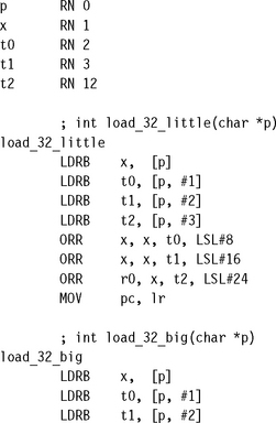
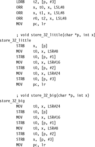
EXAMPLE 6.30
This example shows how to read or write a 32-bit word using the unaligned address p. We use three scratch registers t0, t1, t2 to avoid interlocks. All unaligned word operations take seven cycles on an ARM9TDMI. Note that we need separate functions for 32-bit words stored in big- or little-endian format.
If you require better performance than seven cycles per access, then you can write several variants of the routine, with each variant handling a different address alignment. This reduces the cost of the unaligned access to three cycles: the word load and the two arithmetic instructions required to join values together.
EXAMPLE 6.31
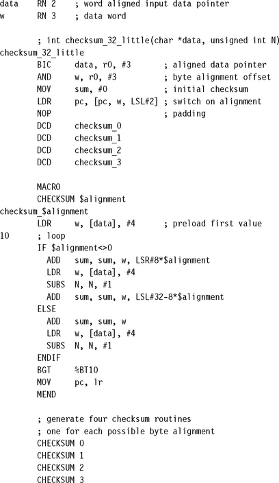
This example shows how to generate a checksum of N words starting at a possibly unaligned address data. The code is written for a little-endian memory system. Notice how we can use the assembler MACRO directive to generate the four routines checksum_0, checksum_1, checksum_2, and checksum_3. Routine checksum_a handles the case where data is an address of the form 4q + a.
Using a macro saves programming effort. We need only write a single macro and instantiate it four times to implement our four checksum routines.
![]()
You can now unroll and optimize the routines as in Section 6.6.2 to achieve the fastest speed. Due to the additional code size, only use the preceding technique for time-critical routines.
SUMMARY: Handling Unaligned Data
![]() If performance is not an issue, access unaligned data using multiple byte loads and stores. This approach accesses data of a given endianness regardless of the pointer alignment and the configured endianness of the memory system.
If performance is not an issue, access unaligned data using multiple byte loads and stores. This approach accesses data of a given endianness regardless of the pointer alignment and the configured endianness of the memory system.
![]() If performance is an issue, then use multiple routines, with a different routine optimized for each possible array alignment. You can use the assembler MACRO directive to generate these routines automatically.
If performance is an issue, then use multiple routines, with a different routine optimized for each possible array alignment. You can use the assembler MACRO directive to generate these routines automatically.
6.10 SUMMARY
For the best performance in an application you will need to write optimized assembly routines. It is only worth optimizing the key routines that the performance depends on. You can find these using a profiling or cycle counting tool, such as the ARMulator simulator from ARM.
This chapter covered examples and useful techniques for optimizing ARM assembly. Here are the key ideas:
![]() Schedule code so that you do not incur processor interlocks or stalls. Use Appendix D to see how quickly an instruction result is available. Concentrate particularly on load and multiply instructions, which often take a long time to produce results.
Schedule code so that you do not incur processor interlocks or stalls. Use Appendix D to see how quickly an instruction result is available. Concentrate particularly on load and multiply instructions, which often take a long time to produce results.
![]() Hold as much data in the 14 available general-purpose registers as you can. Sometimes it is possible to pack several data items in a single register. Avoid stacking data in the innermost loop.
Hold as much data in the 14 available general-purpose registers as you can. Sometimes it is possible to pack several data items in a single register. Avoid stacking data in the innermost loop.
![]() For small if statements, use conditional data processing operations rather than conditional branches.
For small if statements, use conditional data processing operations rather than conditional branches.
![]() Use unrolled loops that count down to zero for the maximum loop performance.
Use unrolled loops that count down to zero for the maximum loop performance.
![]() For packing and unpacking bit-packed data, use 32-bit register buffers to increase efficiency and reduce memory data bandwidth.
For packing and unpacking bit-packed data, use 32-bit register buffers to increase efficiency and reduce memory data bandwidth.
![]() Use branch tables and hash functions to implement efficient switch statements.
Use branch tables and hash functions to implement efficient switch statements.
![]() To handle unaligned data efficiently, use multiple routines. Optimize each routine for a particular alignment of the input and output arrays. Select between the routines at run time.
To handle unaligned data efficiently, use multiple routines. Optimize each routine for a particular alignment of the input and output arrays. Select between the routines at run time.