
Discrete-Time Signals and Systems
Leonardo G. Baltar and Josef A. Nossek, Institute for Circuit Theory and Signal Processing, Technische Universität München, München, Germany, [email protected], [email protected]
Abstract
In this chapter we will investigate the fundamental topic of discrete-time signals and systems. We first introduce some basic and useful discrete-time signals, like the unit impulse, the sinusoidal and white Gaussian random sequences. Then we define and represent discrete-time systems. We give some criteria with which these systems can be classified. Then for the important class of linear time-invariant (LTI) systems we focus on the state-space description that will form the basis for the analysis on following sections. We define observability and controllability and present how to evaluate the stability of LTI systems. Finally, we give some simple examples how to describe, analyze and implement discrete-time signals and systems in MATLAB.
Keywords
Discrete-time systems; Sequences; LTI systems; State-space description; Difference equations; Stability
1.03.1 Introduction
Discrete-time systems are signal processing entities that process discrete-time signals, i.e., sequences of signal values that are generally obtained as equidistant samples of continuous-time waveforms along the time axis. Usually a clock signal will determine the period T (sampling interval) in which the input signal values enter the system and, respectively, the output samples leave the system. The interval T also determines the cycle in which the internal signal values within the system are processed. Typical representatives of this class of systems are the analog discrete-time signal processing systems (switched capacitor circuits, charge-coupled devices (CCD), bucket-brigade devices (BBD)) as well as digital systems. In the case of the last, the sequence value for each sampling interval will also be discretized, i.e., it will be represented with a finite set of amplitudes, usually in a binary representation. Chapter 5 covers the topic of sampling and quantization of continuous-time signals.
It is worth mentioning, that in the case of multi-rate discrete-time systems, the interval in which the internal signals and possibly the output signal are processed will usually be different from T. The topic of multi-rate discrete-time systems is covered in Chapter 9.
It is important to emphasize that the discussion in this chapter considers the special case of discrete-time signals with unquantized values. This means that the amplitude of all the signals and the value of the parameters (coefficients) that describe the discrete-time systems are represented with infinite word length. This is an abstraction from real digital signals and systems, where the finite word length representation of both signals and parameters have to be taken into account to fully cover all important phenomena, such as limit cycles. Design of digital filters and their implementation will be discussed in Chapter 7.
1.03.2 Discrete-time signals: sequences
Discrete-time signals can arise naturally in situations where the data to be processed is inherently discrete in time, like in financial or social sciences, economy, etc. Generally, the physical quantities that the discrete-time signal represents evolve continuously over time (for example, voice, temperature, voltages, currents or scattering variables), but inside a sampling interval of T seconds, can be completely characterized by means of a single value only, see Figure 3.1. In the last case, the continuous-time signals are first sampled or discretized over time and possibly also quantized in amplitude.

Still images are usually described as two dimensional discrete signals, where the two dimensions are spatial dimensions. For moving images, a third dimension is added.
Important examples of discrete-time signals that are used in practice are addressed in the following.
Analogously to the continuous-time unit impulse, known as the Dirac delta function, we can also define a discrete-time unit impulse, known as the Kronecker delta function, as
 (3.1)
(3.1)
where n is an integer number. The discrete time unit impulse is graphically shown in Figure 3.2. Any arbitrary discrete time sequence can be represented as a sum of weighted and delayed unit impulses. Also analogous to the continuous-time systems, the input–output behavior of a discrete-time system can also be described by the impulse response, as we will see in details in a later section.

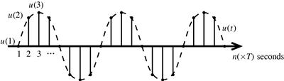
Another commonly used test signal is a sequence, where the samples are equidistantly taken from a sinusoid
![]() (3.2)
(3.2)
with U and ![]() being real constants.
being real constants. ![]() is the frequency of the sinusoid in rad/s. In some cases it is important to analyze a system for certain frequencies and in this case a sinusoid input with the frequencies of interest can be applied at the input. An example of a discrete-time sinusoid and the corresponding continuous-time waveform are depicted in Figure 3.3
is the frequency of the sinusoid in rad/s. In some cases it is important to analyze a system for certain frequencies and in this case a sinusoid input with the frequencies of interest can be applied at the input. An example of a discrete-time sinusoid and the corresponding continuous-time waveform are depicted in Figure 3.3
We can also define a random sequence, an example being the case where the samples are distributed according to a normal distribution with zero mean and given variance ![]() and the individual samples are statistically independent, i.e.,
and the individual samples are statistically independent, i.e.,
 (3.3)
(3.3)
This is the discrete equivalent of the white Gaussian noise and it is useful if the behavior of the discrete time system is to be analyzed for all frequencies at once. Also in the case where some noise sources are to be included during the analysis or modeling of a discrete-time system implementation, this random sequence is the most used one. See Chapter 4 for more details on random sequences.
1.03.3 Discrete-time systems
A discrete-time system with discrete-time input sequence ![]() and output sequence
and output sequence ![]() is an operator
is an operator ![]() that performs the mapping
that performs the mapping
![]() (3.4)
(3.4)
It is important to note that this mapping is applied to the entire input sequence ![]() , beginning with some starting instant in the far distant past, including the present instant n and up to a far future instant, to obtain the present output
, beginning with some starting instant in the far distant past, including the present instant n and up to a far future instant, to obtain the present output ![]() .
.
1.03.3.1 Classification
There are many different classes of discrete-time systems. They can be categorized according to various important properties that will allow us to analyze and design systems using specific mathematical tools. All the properties explained here find an equivalent for continuous-time systems.
1.03.3.1.1 Memoryless systems
One sample of the output sequence ![]() of a memoryless system for a specific index
of a memoryless system for a specific index ![]() depends exclusively on the input value
depends exclusively on the input value ![]() . The output depends neither on any past or future value of the input
. The output depends neither on any past or future value of the input ![]() nor on any past or future value of the output
nor on any past or future value of the output ![]() , i.e.,
, i.e.,
![]() (3.5)
(3.5)
1.03.3.1.2 Dynamic systems
In contrast, a memory or dynamic system has its output dependent on at least one past value, either the output or the input
![]() (3.6)
(3.6)
The positive integer constant N is usually called the degree of the system. We have assumed here, without loss of generality, that the same number of past inputs and outputs influence a certain output sample.
1.03.3.1.3 Linear systems
If the system is a linear system, the superposition principle should hold. Let us consider an input ![]() for the system. Then the output is
for the system. Then the output is
![]() (3.7)
(3.7)
Similarly, with another input ![]() , the output is
, the output is
![]() (3.8)
(3.8)
The superposition principle tells us that if each input is scaled by any constant ![]() , and moreover, the sum of the inputs is employed as a new input, then for the new output, it holds that
, and moreover, the sum of the inputs is employed as a new input, then for the new output, it holds that
![]() (3.9)
(3.9)
This can be extended for any number of different inputs and any value of the scaling factors. One of the simplest and probably most popular linear dynamic system is the recurrence used to generate Fibonacci sequences [1]:
![]() (3.10)
(3.10)
where ![]() .
.
1.03.3.1.4 Non-linear systems
In the case of non-linear systems, the superposition principle does not apply. An example of this is the famous logistic map [2] or discrete logistic equation, that arise in many contexts in the biological, economical and social sciences.
![]() (3.11)
(3.11)
where ![]() is a positive real number,
is a positive real number, ![]() and
and ![]() represents a initial ratio of population to a maximum population. The logistic map is a discrete-time demographic model analogous to the continuous-time logistic equation [3] and is a simple example of how chaotic behavior can arise. In this chapter we are mainly interested in linear systems, since there exist many well established analysis tools.
represents a initial ratio of population to a maximum population. The logistic map is a discrete-time demographic model analogous to the continuous-time logistic equation [3] and is a simple example of how chaotic behavior can arise. In this chapter we are mainly interested in linear systems, since there exist many well established analysis tools.
1.03.3.1.5 Time-invariant systems
If the samples of the input sequence are delayed by ![]() and the output samples are delayed by the same interval, a discrete-time system is called time-invariant.
and the output samples are delayed by the same interval, a discrete-time system is called time-invariant.
![]() (3.12)
(3.12)
Both the Fibonacci recurrence and the logistic map are Time-invariant systems.
1.03.3.1.6 Time-variant systems
In the case of time-variant systems, internal parameters of the system, like multiplier coefficients, can also vary with time. This is the case for the so-called adaptive systems or adaptive filters (see Chapter 11 for more details). A simple example of a time-variant system is the amplitude modulation
![]() (3.13)
(3.13)
There exists a special case of time-variant systems where the internal multiplier coefficients do not necessarily vary with time, but the sampling rate is changed within the system. Those systems are called multi-rate systems and they frequently present a cyclical output. This means that for a certain multiple delay of the input signal, the output sequence will have the same samples as for the non-delayed input.
1.03.3.1.7 Causal systems
In a causal system, the output samples only depend on the actual or past samples of the input sequence, and on past samples of the output itself. If the system is non-causal, it means that the output sample depends on an input value that has not yet entered the system. The definition of dynamic systems in (1.03.3.1) is already considered a causal case. Non-causal systems are not relevant for almost all practical applications.
1.03.4 Linear time-invariant (LTI) systems
This is a technically important class of discrete-time systems, for which a rich mathematical framework exists.
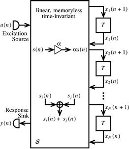
Linear time-invariant continuous-time systems in the electrical/electronic domain can be built with memoryless (resistive) elements such as resistors, independent and controlled sources and memory possessing (reactive) elements, for example, capacitors or inductors. In linear time-invariant discrete-time systems, we also have memoryless and memory-possessing elements such as
The symbolic representations of these aforementioned elements are depicted in Figure 3.4. It is important to note that in this context, nothing is said about how these elements are realized—neither with which electronic components nor with which technology.

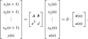
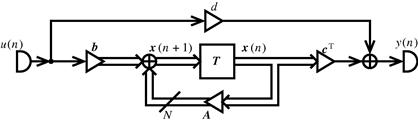
1.03.4.1 State-space description
Any linear time-invariant system can be structured into a memoryless linear ![]() terminal network with N delay elements and a single input and a single output. Although the system can easily extend to multiple inputs and/or multiple outputs, we will consider only single input/single output (SISO) systems, with which we can study all important phenomena.
terminal network with N delay elements and a single input and a single output. Although the system can easily extend to multiple inputs and/or multiple outputs, we will consider only single input/single output (SISO) systems, with which we can study all important phenomena.
Because everything within the linear time-invariant memoryless box in Figure 3.5 can only perform weighted sums, the ![]() dimensional input vector (state vector
dimensional input vector (state vector ![]() stacked with scalar input
stacked with scalar input ![]() ) is mapped onto the
) is mapped onto the ![]() dimensional output vector (state vector
dimensional output vector (state vector ![]() stacked with scalar output
stacked with scalar output ![]() ) through multiplication with the
) through multiplication with the ![]() matrix
matrix ![]()
 (3.14)
The matrix ![]() can obviously be partitioned into the well-known state space description
can obviously be partitioned into the well-known state space description
![]() (3.15)
(3.15)
where ![]() .
.
Now we can take (3.15) and refine the block diagram depicted in Figure 3.5 to show Figure 3.6, which is the general state-space realization. The structure in Figure 3.6 is still rather general, because for each element of ![]() and d, a multiplication has to be performed, especially if we assume all of their elements with non-trivial values. The total number of multiplications is in this case,
and d, a multiplication has to be performed, especially if we assume all of their elements with non-trivial values. The total number of multiplications is in this case, ![]() . But, as we will see later, that
. But, as we will see later, that ![]() and
and ![]() are not uniquely determined by a given input–output mapping. Consequently there is room for optimization, e.g., to reduce the number of actual multiplications to be performed per sample.
are not uniquely determined by a given input–output mapping. Consequently there is room for optimization, e.g., to reduce the number of actual multiplications to be performed per sample.
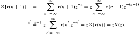
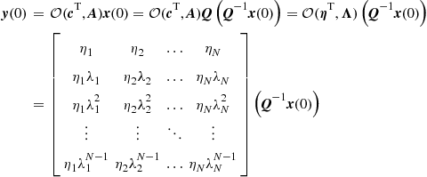
Let us compute the output signal ![]() , using an initial state vector
, using an initial state vector ![]() , and the input signal sequence from the time instant
, and the input signal sequence from the time instant ![]() onwards
onwards
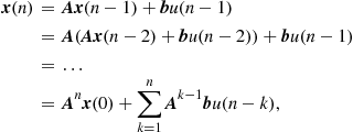 (3.16)
 (3.17)
From this general response we can also derive the so-called impulse response, for which we set ![]() and
and ![]() , the unit impulse which was defined in (3.1). This leads to
, the unit impulse which was defined in (3.1). This leads to
 (3.18)
By making use of the impulse response ![]() , we can reformulate the zero-state response with a general input sequence
, we can reformulate the zero-state response with a general input sequence ![]()
 (3.19)
which is the so-called convolution sum. This summation formulation is corresponding to the so-called convolution integral for continuous-time signals and systems.
Now it is time to show that we can generate a whole class of equivalent systems (equivalent in the sense that they have the same zero-state response and the same input-output mapping respectively) with the aid of a so-called similarity transform.
With a non-singular ![]() matrix
matrix ![]() we can define a new state vector as the linear transformation of the original one as
we can define a new state vector as the linear transformation of the original one as ![]() , then we can rewrite the state-space equations with the new state vector
, then we can rewrite the state-space equations with the new state vector ![]() as
as
![]() (3.20)
(3.20)
and by multiplying the first equation with ![]() from the left side we get
from the left side we get
![]() (3.21)
(3.21)
The new state-space representation can now be formulated as
![]() (3.22)
(3.22)
where the equations
![]() (3.23)
(3.23)
By inserting ![]() and
and ![]() into the zero-state response, we see that this response is invariant to the above transformation.
into the zero-state response, we see that this response is invariant to the above transformation.
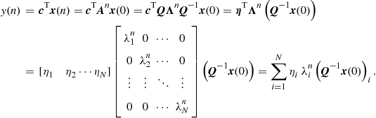
Depending on the choice of the transformation matrix, the matrix ![]() can have different forms. A particularly interesting form is the so-called normal form, where the state matrix is diagonalized, allowing a much lower complexity than a dense matrix. First we apply an eigenvalue decomposition [4] to
can have different forms. A particularly interesting form is the so-called normal form, where the state matrix is diagonalized, allowing a much lower complexity than a dense matrix. First we apply an eigenvalue decomposition [4] to ![]() :
:
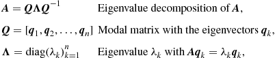
where we have assumed that ![]() is diagonalizable and we do not need to resort to the Jordan form. The transformation matrix and the new state vector are
is diagonalizable and we do not need to resort to the Jordan form. The transformation matrix and the new state vector are ![]() and
and ![]() . The system can then be described by
. The system can then be described by
![]() (3.24)
(3.24)
which leads to the new specific implementation of Figure 3.7. With this new implementation, the number of coefficients, and consequently the number of multiplications, is reduced to ![]() .
.

If some of the eigenvalues are complex valued (if this is the case they will always come in complex conjugate pairs provided ![]() is real valued), we always will merge the two corresponding first order systems to one second order system with real valued multiplier coefficients only. This is equivalent to have a block diagonal state matrix (with 2-by-2 blocks) instead of a diagonal one.
is real valued), we always will merge the two corresponding first order systems to one second order system with real valued multiplier coefficients only. This is equivalent to have a block diagonal state matrix (with 2-by-2 blocks) instead of a diagonal one.
Now we can compute the transfer function by transforming (3.15) to the frequency domain with the ![]() -transform.
-transform.
1.03.4.2 Transfer function of a discrete-time LTI system
Similar to continuous-time systems we can also analyze a discrete-time system with the help of a functional transform to make a transition to the frequency domain. However, we have only sequences of signal values in the time domain and not continuous waveforms. Therefore, we have to apply the ![]() -transform [5]:
-transform [5]:
 (3.25)
The delay in the time-domain is represented in the frequency domain by a multiplication by ![]() .
.
 (3.26)
Now we can transform the state-space equations to the frequency domain
![]() (3.27)
(3.27)
and after we eliminate the state vector ![]() , we obtain the transfer function
, we obtain the transfer function
![]() (3.28)
(3.28)
Since
![]() (3.29)
(3.29)
holds, ![]() is obviously a periodical function of
is obviously a periodical function of ![]() resp. f with frequency-period
resp. f with frequency-period ![]() resp.
resp. ![]() .
.
The question that arises here is: What type of function is (3.28)? To answer that we have to consider the expression ![]() more closely. We assume of course that
more closely. We assume of course that ![]() is nonsingular and therefore the inverse exists (this means that the inversion will only be performed for the values of z at which it is possible). The inverse reads
is nonsingular and therefore the inverse exists (this means that the inversion will only be performed for the values of z at which it is possible). The inverse reads
![]() (3.30)
(3.30)
where the determinant is a polynomial in z of degree N, also called the characteristic polynomial
![]() (3.31)
(3.31)
and the elements of the adjugate matrix are the transposed cofactors of the matrix. The cofactors on the other hand are sub-determinants of ![]() and therefore polynomials of at most degree
and therefore polynomials of at most degree ![]() .
.
The numerator of ![]() is hence a linear combination of cofactors, i.e., a linear combination of polynomials of degree
is hence a linear combination of cofactors, i.e., a linear combination of polynomials of degree ![]() and therefore a polynomial of at most degree
and therefore a polynomial of at most degree ![]() . If we apply this result in Eq. (3.28), we will obtain a rational fractional function of z
. If we apply this result in Eq. (3.28), we will obtain a rational fractional function of z
![]() (3.32)
(3.32)
where ![]() only for
only for ![]() , since
, since ![]() .
.
We usually divide the nominator and the denominator by ![]() and obtain in the numerator and in the denominator polynomials in
and obtain in the numerator and in the denominator polynomials in ![]() :
:
 (3.33)
By multiplying both sides of (3.33) with the denominator we get
 (3.34)
Now we go back to the time domain with help of the inverse ![]() -transform and obtain a global difference equation
-transform and obtain a global difference equation
 (3.35)
The difference equation is equivalent to the description of a discrete-time system like a differential equation is for the description of a continuous-time system.
The representation of Eq. (3.35) leads us to an important special case, for which we have no equivalent in continuous-time systems built with lumped elements: the so-called finite impulse (FIR) response systems.
1.03.4.3 Finite duration impulse response systems
Those are systems with, as the name says, a finite duration impulse response (FIR), i.e., the ![]() ’s in (3.35) are equal to zero such that
’s in (3.35) are equal to zero such that
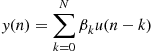 (3.36)
and with a unit impulse as excitation ![]() we get
we get
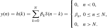 (3.37)
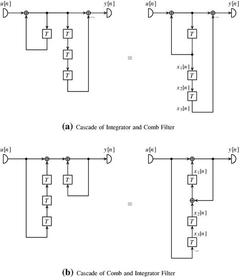
We can see that the coefficients of the polynomial transfer function directly give then values of the impulse response and so that it takes us directly to an implementation, see Figure 3.8. Note that the two structures are inter-convertible if the principle of flow reversal is applied to the block diagram.

Let us now write down the state space description for the uppermost structure in Figure 3.8. By calling the input of the delay elements ![]() and their outputs
and their outputs ![]() indexing them from the left most to the rightmost we can see that
indexing them from the left most to the rightmost we can see that
 (3.38)
and for the output
![]() (3.39)
(3.39)
holds. In matrix vector notation we get
 (3.40)
![]() (3.41)
(3.41)
It can be easily demonstrated that the second structure in Figure 3.8 is obtained by a transposition of the state-space description of the first structure, the matrix and vectors for it are then given by
![]() (3.42)
(3.42)
Other usual names for FIR systems are:
1.03.4.4 Infinite duration impulse response systems
On the other hand if the ![]() ’s are different from zero, then the impulse response will have infinite duration, as the name says. We can again clearly derive a realization structure from the corresponding time-domain description, in this case from Eq. (3.35), see Figure 3.9. This per se inefficient realization (two times the number of necessary delay elements) can be transformed into the well known direct form through simple rearranging the two blocks like in Figure 3.10. This is called a canonical realization because it possesses a minimum number of delay elements.
’s are different from zero, then the impulse response will have infinite duration, as the name says. We can again clearly derive a realization structure from the corresponding time-domain description, in this case from Eq. (3.35), see Figure 3.9. This per se inefficient realization (two times the number of necessary delay elements) can be transformed into the well known direct form through simple rearranging the two blocks like in Figure 3.10. This is called a canonical realization because it possesses a minimum number of delay elements.
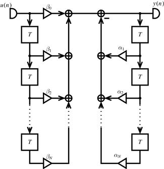
Figure 3.9 IIR realization according to Eq. (3.35).

Now we can setup the state-space equations for the IIR system structure of Figure 3.10. As already mentioned we label the output of the delays the states ![]() and their inputs
and their inputs ![]() . By numbering from the topmost to the lowest delay we can see that
. By numbering from the topmost to the lowest delay we can see that
![]() (3.43)
(3.43)
holds and from the second until the Nth-state we get
 (3.44)
For the output we can see that
![]() (3.45)
(3.45)
where we have used the definition of ![]() of (3.43). In matrix vector notation we get
of (3.43). In matrix vector notation we get
 (3.46)
![]() (3.47)
(3.47)
where because of its particular structure, ![]() is called a companion matrix.
is called a companion matrix.
If we apply the principle of flow reversal to the diagram of Figure 3.10 we will end up with the realization shown in Figure 3.11. This is again equivalent to transform the state-space description into the transposed system, i.e., the transformed system is represented by
![]() (3.48)
(3.48)
If we apply these definitions to (3.28) we can see that
 (3.49)
This means that the transposed realization has the same transfer function as the original system.
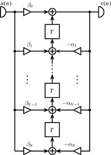
Figure 3.11 Transposed realization of the system from Figure 3.10.
Other usual names for IIR systems are:
1.03.4.5 Observability and controllability
As we have seen in the previous section every LTI system can be completely characterized by a state-space description
![]() (3.50)
(3.50)
![]() (3.51)
(3.51)
from which we can uniquely derive the corresponding transfer function
![]() (3.52)
(3.52)
It is important to note that although the way from a given state-space description to the input–output transfer function is unique, the same is not true for the other direction. For one given transfer function there are infinitely many different state-space realizations, which all may have a number of different properties, with the very same input–output relation. One of those properties is the stability of the so-called LTI system.
An often applied stability criterion is to check whether the zeroes of the denominator polynomial of the transfer function ![]() lie within the unit circle of the z-plane or equivalently the impulse response
lie within the unit circle of the z-plane or equivalently the impulse response
![]() (3.53)
(3.53)
decays over time. In the following we will see that this is not telling us the complete truth about the stability of LTI systems. Because stability depends on the actual implementation, which in detail is reflected in the state-space description and not only in transfer function or impulse response. To get a clear view, we have to introduce the concept of observability and controllability, and based on these concepts define different types of stability.
Let us start with the definition of observability.
Starting with the state-space description (3.50) we assume that the excitation ![]() for
for ![]() and an initial state
and an initial state ![]() . Let us now compute the system output in time domain:
. Let us now compute the system output in time domain:
 (3.54)
Let us stack these subsequent N output values in one vector
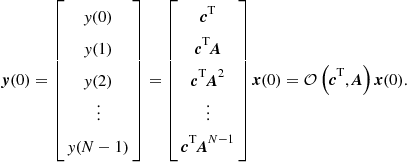 (3.55)
From (3.55) we see that this output vector ![]() is given by the product of the so called observability matrix
is given by the product of the so called observability matrix ![]() , which is completely determined by
, which is completely determined by ![]() and
and ![]() and the system state at the time instant
and the system state at the time instant ![]() . Now if the observability matrix is invertible, we can compute the state vector
. Now if the observability matrix is invertible, we can compute the state vector
![]() (3.56)
(3.56)
If this is possible, the system (3.50) is completely observable.
Next we define controllability in a corresponding way by assuming an initial zero state ![]() and let us look for a sequence
and let us look for a sequence ![]() to drive the system into some desired state
to drive the system into some desired state ![]() . We look at the evolution of the state as controlled by the excitation
. We look at the evolution of the state as controlled by the excitation
 (3.57)
This can be put together as
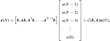 (3.58)
where ![]() is the so called controllability matrix and
is the so called controllability matrix and ![]() is the vector, in which the subsequent excitation samples have been stacked. If the controllability matrix is invertible, we can solve for the excitation
is the vector, in which the subsequent excitation samples have been stacked. If the controllability matrix is invertible, we can solve for the excitation
![]() (3.59)
(3.59)
which will steer the system from the zero initial state into a specified desired state ![]() . If this is possible, the system (3.50) is completely controllable.
. If this is possible, the system (3.50) is completely controllable.
1.03.4.6 Stability
Based on the concepts of observability and controllability we can now define different concepts of stability:
We will start with internal stability by requiring that the Euclidean norm of the state vector hat to decay over time from any initial value with zero excitation:
![]() (3.60)
(3.60)
This is equivalent to require the state vector converge to the zero vector.
By looking at the evolution of the state vector over time
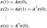 (3.61)
and making use of the eigenvalue decomposition (EVD) of ![]() we get
we get
![]() (3.62)
(3.62)
From (3.62) we can conclude that the vector ![]() will converge to the zero vector, i.e.,
will converge to the zero vector, i.e., ![]() if and only if all eigenvalues
if and only if all eigenvalues ![]() of
of ![]() are smaller than one in magnitude
are smaller than one in magnitude
![]() (3.63)
(3.63)
This equivalent to say that the poles of the transfer function are localized inside the unity circle, since the eigenvalues of ![]() equal to the poles of the transfer function. In the above derivation we have assumed that
equal to the poles of the transfer function. In the above derivation we have assumed that ![]() is a diagonalizable matrix. If this is not the case because of multiples eigenvalues, we have to refrain to the so called Jordan form. Although this is slightly more complicated, it leads to the same result.
is a diagonalizable matrix. If this is not the case because of multiples eigenvalues, we have to refrain to the so called Jordan form. Although this is slightly more complicated, it leads to the same result.
A somewhat weaker stability criterion is to check only if the system output decays to zero from any initial state and zero excitation:
![]() (3.64)
(3.64)
Computing the output we get
 (3.65)
![]() is the transformed output vector. If an entry
is the transformed output vector. If an entry ![]() is equal to zero, then the eigenmode (normal mode)
is equal to zero, then the eigenmode (normal mode) ![]() will not contribute to the system output and, therefore, a non-decaying eigenmode
will not contribute to the system output and, therefore, a non-decaying eigenmode ![]() will not violate the output-stability criterion. This can only happen if the observability matrix is not full rank. From (3.55) we have
will not violate the output-stability criterion. This can only happen if the observability matrix is not full rank. From (3.55) we have
 (3.66)
and that ![]() is rank deficient if a least one
is rank deficient if a least one ![]() is zero, and since
is zero, and since ![]() is full rank
is full rank ![]() must also be rank deficient. Therefore, a system can be output stable without being internally stable, if it is not completely observable.
must also be rank deficient. Therefore, a system can be output stable without being internally stable, if it is not completely observable.
A complementary criterion is that of input-stability, requiring the state vector converging to the zero vector, but not from any arbitrary initial state, but only from states which can be controlled from the system input. Now we start with an initial state ![]() , which can be generated from an input sequence (see (3.58))
, which can be generated from an input sequence (see (3.58))
![]() (3.67)
(3.67)
The transformed state ![]() then reads
then reads
![]() (3.68)
(3.68)
with the transformed input vector ![]() . After the input
. After the input ![]() has produced the state
has produced the state ![]() it is switched off, i.e.
it is switched off, i.e. ![]() for
for ![]() .
.
We ask whether the state vector can converge to the zero vector although the system may not be internally stable. The answer is given by the structure of
 (3.69)
If some ![]() , then
, then ![]() will converge to the zero vector, even if the corresponding
will converge to the zero vector, even if the corresponding ![]() , because this non-decaying eigenmode cannot be excited from the regular input. But this is only possible, if
, because this non-decaying eigenmode cannot be excited from the regular input. But this is only possible, if ![]() is not full rank and the system is, therefore, not completely controllable.
is not full rank and the system is, therefore, not completely controllable.
Finally we look at the concept of the commonly used input–output-stability, i.e., we excite the system with zero initial state with a unit pulse and require the output to converge to zero over time. In this setting the state and the output evolves as
![]() (3.70)
(3.70)
 (3.71)
The output will converge to zero, even if there are non-decaying eigenmodes ![]() , as long as for every such
, as long as for every such ![]() there is a
there is a ![]() or a
or a ![]() , or both are zero. We see that a system could be input–output stable, although it is neither internally stable nor input- or output-stable.
, or both are zero. We see that a system could be input–output stable, although it is neither internally stable nor input- or output-stable.
Only for systems, which are completely observable and controllable, the four different stability criteria coincide.
Example: 3.1
The four stability concepts will now be illustrated with an example: the Cascade Integrator Comb (CIC) filter [6]. These filters are attractive in situations where either a narrow-band signal should be extracted from a wideband source or a wideband signal should be constructed from a narrowband source. The first situation is associated with the concept of sampling rate decrease or decimation and the second one leads to the concept of sampling rate increase or interpolation. CIC filters are very efficient from a hardware point of view, because they need no multipliers. In the first case, i.e., decimation, the integrators come first, then the sampling rate will be decreased by a factor of R followed by a subsequent cascade of comb filters (Figure 3.12a), while in the second case, i.e., interpolation, the comb filters come first, then the sampling rate increase is followed by a subsequent cascade of integrators (Figure 3.12b).

The stability problem in these CIC filters stems from the integrators, which obviously exhibit a non-decaying eigenmode (pole with unit magnitude). To analyze the stability of such CIC filters we set the sampling rate decrease/increase factor ![]() and the number of integrators and comb filters stages to
and the number of integrators and comb filters stages to ![]() without loss of generality. In addition we assume a differential delay of
without loss of generality. In addition we assume a differential delay of ![]() samples per stage. This leads us to the following two implementations to be analyzed which are shown in Figures 3.13a and b.
samples per stage. This leads us to the following two implementations to be analyzed which are shown in Figures 3.13a and b.
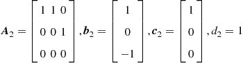
Let us start with an analysis of the filter in Figure 3.13a, the state space description of which reads
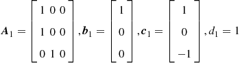 (3.72)
and leads to the transfer function
![]() (3.73)
(3.73)
The observability matrix
 (3.74)
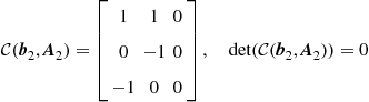
is obviously rank deficient and the system is therefore not completely observable.
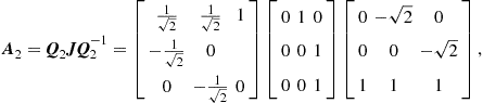
Since the state matrix ![]() is not diagonalizable, we have to refrain to a Jordan form
is not diagonalizable, we have to refrain to a Jordan form
 (3.75)
which shows the three eigenvalues are ![]() and
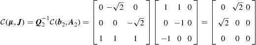
and ![]() . Not all eigenvalues are less then one in magnitude. Therefore, the system of Figure 3.13a is not internaly stable. But transforming the observability matrix according to (3.66), we get
. Not all eigenvalues are less then one in magnitude. Therefore, the system of Figure 3.13a is not internaly stable. But transforming the observability matrix according to (3.66), we get
 (3.76)
with the third component ![]() of the transformed output vector
of the transformed output vector ![]() equal to zero. This clearly means that the non-vanishing third eigenmode is not observable at the system output. Therefore the system is output stable, i.e., the output converges in the limit
equal to zero. This clearly means that the non-vanishing third eigenmode is not observable at the system output. Therefore the system is output stable, i.e., the output converges in the limit ![]() y (n)=0, although the state vector does not converge to the zero vector. But the controllability matrix
y (n)=0, although the state vector does not converge to the zero vector. But the controllability matrix
 (3.77)
is full rank, i.e., the system is completely controllable, and an arbitrary input sequence may excite the non-decaying eigenmode. Therefore, the system is not input-stable.
Now let us analyze the filter in Figure 3.13b, which has the following state-space description
 (3.78)
and the same transfer function as the previous filter from Figure 3.13a. It is interesting to note that the second filter can be obtained from the first one by applying transposition
![]() (3.79)
(3.79)
The controllability matrix of the second system
 (3.80)
is obviously rank deficient and the system is therefore not completely controllable.
Since the state matrix ![]() is not diagonalizable we have again to refrain to a Jordan form
is not diagonalizable we have again to refrain to a Jordan form
 (3.81)
which again shows obviously the same eigenvalues ![]() and
and ![]() . The second system is again not internally stable. Transforming the above controllability matrix according to (3.68) we get
. The second system is again not internally stable. Transforming the above controllability matrix according to (3.68) we get
 (3.82)
with the third component ![]() of the transformed input vector
of the transformed input vector ![]() being equal to zero. This shows that the non-decaying third eigenmode will not be excited by any possible input signal. Therefore, the system is input-stable, although it is not internaly stable.
being equal to zero. This shows that the non-decaying third eigenmode will not be excited by any possible input signal. Therefore, the system is input-stable, although it is not internaly stable.
The observability matrix of the second system
 (3.83)
is full rank and the second system is completely observable. Therefore the non-decaying eigenmode, although not excited by any input sequence, is observable at the output. This can always happen because of an unfavorable initial state accidentally occurring in the switch-on transient of the power supply or because of some disturbance entering the system not through the regular input path. Therefore, the system is not output-stable.
But both systems are input–output-stable, because both have the same impulse response with finite duration.
This example shows, that the standard input–output stability criterion, i.e., requiring a decaying impulse response, is not always telling the whole story. Judging whether a system is stable or not needs a detailed knowledge about the system structure, or in other words the realization, and not only about input–output-mapping.
1.03.5 Discrete-time signals and systems with MATLAB
In this section we will provide some examples how to generate discrete-time signals in MATLAB and how to represent and implement basic discrete-time systems. We assume here a basic MATLAB installation. The commands and programs shown here are not unique in the way they perform the analysis and implement discrete-time signals and systems. Our objective here is to give an introduction with very simple commands and functions. With this introduction the reader will get more familiar with this powerful tool that is widely employed to analyze, simulate and implement digital signal processing systems. If one has access to the full palette of MATLAB toolboxes, like e.g., Signal Processing Toolbox, Control System Toolbox, Communications System Toolbox and DSP System Toolbox, many of the scripts included here can be substituted by functions encountered in those libraries.
1.03.5.1 Discrete-time signals
Discrete-time signals are defined in MATLAB as one dimensional arrays, i.e., as vectors. They can be row or column vectors and their entries can be either real or complex valued. The signals we will generate and analyze in this section are always row vectors and their entries are always real valued. The length of the vectors will be defined according to the time span in which the system is supposed to be analyzed.
1.03.5.1.1 Unit impulse
The unit impulse ![]() can be generated with the commands
can be generated with the commands
where L is the length of the desired input and the function zeros(1,L-1) generates a row vector with L-1 zeros.
The unit impulse can be further weighted and delayed. For example, ![]() can be generated by
can be generated by
where we have assumed a delay of 5 samples or sampling periods.
The length of the vector containing only a unit impulse depends on the objective of the analysis. For example, if the impulse response of a discrete-time system is to be studied, there should be enough elements in the input array so that a significant part of the impulse response is contained in the output vector.
1.03.5.1.2 Sinusoid
A sinusoid can be generated with the help of the function sin. Below is an example of a sinusoid where all its parameters are first defined
| fs = 1000; | % Sampling frequency in Hz |
| T = 1/fs; | % Sampling period |
| n = 1:100; | % Time indexes |
| U = 0.5; | % Amplitude of the sinusoid |
| fc = 20; | % Sinusoid frequency in Herz |
| omega = 2* pi* fc; | % Sinusoid angular frequency in rad/s |
| phi = 0; | % phase in radians |
| x = U* sin (omega* n* T+phi); |
We can see that the comments after each command explain what the parameter means.
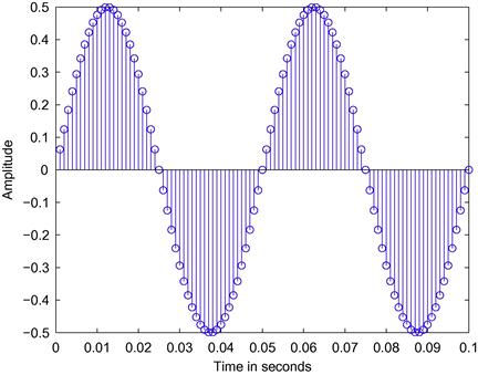
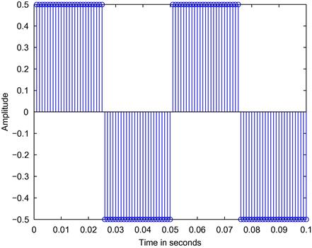
If we would like to graphically represent the sinusoid, we could use
and we get the plot in Figure 3.14, where we can see two periods of the sinusoid. An alternative to stem is the command plot. If we employ it using the same parameters and the same syntax we obtain Figure 3.15, where it should be noted that MATLAB graphically connects the amplitude samples with a straight line and as a consequence the discrete-time sinusoid looks like a continuous-time one. It is important to keep in mind that the true discrete-time sinusoid is only defined for certain time instants and the amplitude between two true samples in the Figure 3.15 is only an approximation of the amplitude of the equivalent continuous-time sinusoid.

As an exercise the reader could play around with the parameters of the sinusoid. For example, he or she could change the phase ![]() to
to ![]() and plot the sinusoid again, then try to use the function cos instead of sin and set
and plot the sinusoid again, then try to use the function cos instead of sin and set ![]() to 0 again and compare with the previous plots. Change the sinusoid frequency until you reach the Nyquist frequency, which is 500 Hz for the example above. Compare the use of the command plot for different sampling rates and different sinusoid frequencies to see how the approximation of the continuous-time sinusoid gets worse.
to 0 again and compare with the previous plots. Change the sinusoid frequency until you reach the Nyquist frequency, which is 500 Hz for the example above. Compare the use of the command plot for different sampling rates and different sinusoid frequencies to see how the approximation of the continuous-time sinusoid gets worse.
1.03.5.1.3 White gaussian noise
To generate a WGN signal we have to employ the function randn that generates pseudo-random numbers following the normal or Gaussian distribution with zero mean and unit variance. By using
we generate a white Gaussian noise vector with zero mean and variance ![]() .
.
1.03.5.1.4 Elaborated signal model
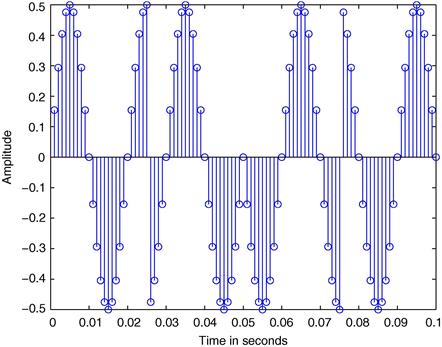
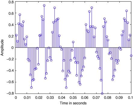
Many operations can be further performed with the generated signals, they can be, for example, added to each other or be multiplied by a constant or by another signal. As a last example let us generate a typical signal model used in communications systems. Let us consider an input signal composed by a sum of weighted and delayed unit impulses. This could be a data carrying signal generated at the transmitter. Then we multiply it by a sinusoid, that could represent a modulation to a higher frequency, for example the radio frequency (RF), to allow the propagation of the signal as an electromagnetic wave in a physical medium between transmitter and receiver. Finally, we add white Gaussian noise that represents the thermal noise generated by the analog components used in the transmitter and receiver.
The program to generate this signal is the following

In Figure 3.16 we can see the signal that is composed by a sum of weighted and delayed unit impulses.
In Figure 3.17 the modulated sinusoid is depicted.
We can see in Figure 3.18 the modulated sinusoid with the additive white Gaussian noise.
1.03.5.2 Discrete-time systems representation and implementation
There are different ways to represent a discrete-time system in MATLAB, like, for example, the space-state or the transfer function. To start we revisit the elaborated signal model introduced in the last section. If we would like to, at least approximately, recover the input signal represented by the sum of delayed and weighted unit impulses, we should first demodulate it by multiplying it by a sinusoid with the same frequency of the one used to modulate
We will then obtain the sequence shown in Figure 3.19.

The only problem with the new sequence is that not only an approximation of the desired signal is obtained, but also another modulated version of it, but this time with a sinusoid with the double of the original modulation frequency, and we still have the additive noise. If the noise variance is low enough we are still able to approximately recover the original signal without any further processing. But we have first to eliminate the modulated signal component and for this we will apply a discrete-time filter specific designed for this task. We assume here that the filter is given and we only care on how to represent and implement it. In [7] and the references therein many methods for the design of discrete-time filters can be encountered.
Let us say that a state-space description of the filter is already known and is defined as

where we can identify the companion matrix structure of ![]() .
.
To compute the output of the filter given an initial state and the input signal, the state equations can be directly employed and iteratively calculated as
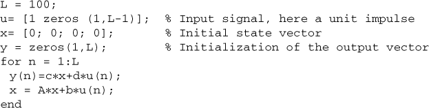
where we can see that the values of the state-vector are not stored for all time instants. If one is interested in looking at the internal states evolution, a matrix could be defined with so many rows as the number of states and so many columns as the length of the input/output signal, and the state vector for each time instant can be saved in its columns.
If we substitute the unit impulse by the demodulated signal as the input u = u_demod we obtain the signal depicted in Figure 3.20. One can see that we do not obtain exactly the input signal u_in but an approximation. particularly in communications systems that is usually the case, where it is important to recover the information contained in u_in, even if the waveform has been distorted, and not the waveform itself.

But if one would like to implement Eq. (3.17) the program becomes more complicated as shown below

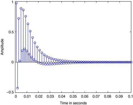
In both programs presented above the impulse response can be obtained and its first 100 samples are plotted in Figure 3.21.
The similarity transformation can also be easily implemented. Let us consider the transformation into the normal form. The code to perform it is
| [Q,Lambda] = eig(A); | % Eigenvalue decomposition: |
| % Lambda -> Eigenvalues in main diagonal | |
| % Q -> Eigenvectors in the columns | |
| T = Q; | |
| A_norm = inv(T)* A* T; | |
| b_norm = inv(T)* b; | |
| c_norm = c* T; | |
| d_norm = d; |
The resulting state-space description for our example is

From the state-space representation it is possible to calculate the coefficients of the numerator and of the denominator polynomials of the transfer function with help of the Faddeev-Leverrier algorithm [8]
where the arrays beta and alpha contain the coefficients of the nominator and denominator polynomials.
With the coefficients of the transfer function it is also possible to calculate the output given the input of the system and some past values of the output by using the difference equation that can be implemented as

As we saw before this equivalent to a state-space realization in direct form.
1.03.6 Conclusion
In this chapter we have introduced an important and fundamental topic in electrical engineering that provides the basics for digital signal processing. We have started with the presentation of some frequently used discrete-time signals. Then we have showed how to classify discrete-time systems and started the study of the widely employed class of linear time-invariant systems. We have showed the most basic way of representing LTI systems in a way that not only the input–output behavior is described, but also important internal signals, the so-called state-space representation. We have seen that the state-space representation is not unique and, consequently, there is room for optimization in the way discrete-time systems are realized. After that, the transfer function was derived from the state-space description and the two main classes of discrete-time systems, namely FIR and IIR were introduced. We formulated the concepts of controllability and observability, and showed how they can be used to evaluate the stability of the system. We finally gave some examples how to implement and analyze simple discrete-time signals and systems with MATLAB.
Relevant Theory: Signal Processing Theory
See this Volume, Chapter 4 Random Signals and Stochastic Processes
See this Volume, Chapter 5 Sampling and Quantization
See this Volume, Chapter 6 Digital Filter Structures and Implementations
See this Volume, Chapter 7 Multirate Signal Processing
See this Volume, Chapter 12 Adaptive Filters
References
1. Wikipedia.Fibonacci number—Wikipedia, the free encyclopedia, 2012 (accessed 16 March 2012).
2. May Robert M. Simple mathematical models with very complicated dynamics. Nature. 1976;261(5560):459–467.
3. Verhulst Pierre-François. Notice sur la loi que la population poursuit dans son accroissement. Correspondance mathématique et physique. 1838;10:113–121.
4. Strang Gilbert. Linear Algebra and Its Applications. third ed. Brooks Cole February 1988.
5. Jury EI. Theory and application of the z-transform method. New York, USA: John Wiley; 1964.
6. Hogenauer EB. An economical class of digital filters for decimation and interpolation. IEEE Trans Acoust Speech Signal Process. 1981;29(2):155–162.
7. da Silva EAB, Diniz PSR, Lima Netto S. Digital Signal Processing: System Analysis and Design. second ed. Cambridge, UK: Cambridge University Press; 2010.
8. Roberts RA, Mullis CT. In: Digital Signal Processing. Addison-Wesley 1987; Number Bd 1 in Addison-Wesley Series in Electrical Engineering.