
Learning Theory
Ambuj Tewari* and Peter L. Bartlett†, *439 West Hall 1085 South University Ann Arbor, MI, USA, †387 Soda Hall #1776 Berkeley, CA, USA, [email protected], [email protected]
Abstract
We present an overview of learning theory including its statistical and computational aspects. We start by giving a probabilistic formulation of learning problems including classification and regression where the learner knows nothing about the probability distribution generating the data. We then consider the principle of empirical risk minimization (ERM) that chooses a function from a given class based on its performance on the observed data. Learning guarantees for ERM are shown to be intimately connected with the uniform law of large numbers. A uniform law of large numbers ensures that empirical means converge to true expectations uniformly over a function class. Tools such as Rademacher complexity, covering numbers, and combinatorial dimensions known as the Vapnik-Chervonenkis (VC) and fat shattering dimensions are introduced. After considering the case of learning using a fixed function class, we turn to the problem of model selection: how to choose a function class from a family based on available data? We also survey alternative techniques for studying generalization ability of learning algorithms including sample compression, algorithmic stability, and the PAC-Bayesian theorem. After dealing with statistical issues, we study computational models of learning such the basic and agnostic PAC learning models, the statistical query, and the mistake bound model. Finally, we point out extensions of the basic theory beyond the probabilistic setting of a learner passively learning a single task from independent and identically distributed samples.
1.14.1 Introduction
In a section on Learning Machines in one of his most famous papers [1], Turing wrote:
Instead of trying to produce a programme to simulate the adult mind, why not rather try to produce one which simulates the child’s? If this were then subjected to an appropriate course of education one would obtain the adult brain. Presumably the child brain is something like a notebook as one buys it from the stationer’s. Rather little mechanism, and lots of blank sheets. (Mechanism and writing are from our point of view almost synonymous.) Our hope is that there is so little mechanism in the child brain that something like it can be easily programmed. The amount of work in the education we can assume, as a first approximation, to be much the same as for the human child.
The year was 1950. Earlier, in 1943, McCulloch and Pitts [2] had already hit upon the idea that mind-like machines could be built by studying how biological nerve cells behave. This directly lead to neural networks. By the late 1950s, Samuels [3] had programmed a machine to play checkers and Rosenblatt [4] had proposed one of earliest models of a learning machine, the perceptron. The importance of the perceptron in the history of learning theory cannot be overemphasized. Vapnik says that the appearance of the perceptron was “when the mathematical analysis of learning processes truly began.” Novikoff’s perceptron theorem (we will prove it in Section 1.14.6.5.2) was also proved in 1962 [5].
Vapnik [6] points out the interesting fact that the 1960s saw four major developments that were to have lasting influence on learning theory. First, Tikhonov and other developed regularization theory for the solution of ill posed inverse problems. Regularization theory has had and continues to have tremendous impact on learning theory. Second, Rosenblatt, Parzen, and Chentsov pioneered nonparametric methods for density estimation. These beginnings were crucial for a distribution free theory of non-parametric classification and regression to emerge later. Third, Vapnik and Chervonenkis proved the uniform law of large numbers for indicators of sets. Fourth, Solomonoff, Kolmogorov, and Chaitin all independently discovered algorithmic complexity: the idea that the complexity of a string of 0’s and 1’s can be defined by the length of the shortest program that can generate that string. This later led Rissanen to propose his Minimum Description Length (MDL) principle.
In 1986, a major technique to learn weights in neural networks was discovered: backpropagation [7]. Around the same time, Valiant [8] published his paper introducing a computational model of learning that was to be called the PAC (probably approximately correct) model later. The 1990s saw the appearance of support vector machines [9] and AdaBoost [10]. This brings us to the brink of the second millenium which is where we end our short history tour.
As we can see, learning theory has absorbed influences from a variety of sources: cybernetics, neuroscience, nonparametric statistics, regularization theory of inverse problems, and the theory of computation and algorithms. Ongoing research is not only trying to overcome known limitations of classic models but is also grappling with new issues such as dealing with privacy and web-scale data.
Learning theory is a formal mathematical theory. Assumptions are made, beautiful lemmas are proved, and deep theorems are discovered. But developments in learning theory also lead to practical algorithms. SVMs and AdaBoost are prime examples of high impact learning algorithms evolving out of a principled and well-founded approach to learning. We remain hopeful that learning theory will help us discover even more exciting learning algorithms in the future.
Finally, a word about the mathematical background needed to read this overview of learning theory. Previous exposure to mathematical reasoning and proofs is a must. So is familiarity with probability theory. But measure theory is not needed as we will avoid all measure-theoretic details. It will also be helpful, but not essential, to be aware of the basics of computational complexity such as the notion of polynomial time computation and NP-completeness. Similarly, knowing a little bit of functional analysis will help.
1.14.2 Probabilistic formulation of learning problems
A basic problem in learning theory is that of learning a functional dependence ![]() from some input space
from some input space![]() to some output or label space
to some output or label space ![]() . Some special choices for the output space deserve particular attention since they arise often in applications. In multiclass classification, we have
. Some special choices for the output space deserve particular attention since they arise often in applications. In multiclass classification, we have ![]() and the goal is to classify any input
and the goal is to classify any input ![]() into one of K given classes. A special case of this problem is when
into one of K given classes. A special case of this problem is when ![]() . Then, the problem is called binary classification and it is mathematically convenient to think of the output space as
. Then, the problem is called binary classification and it is mathematically convenient to think of the output space as ![]() rather than
rather than ![]() . In regression, the output space
. In regression, the output space ![]() is some subset of the set
is some subset of the set ![]() of real numbers. Usually
of real numbers. Usually ![]() is assumed to be a bounded interval, say
is assumed to be a bounded interval, say ![]() .
.
We assume that there is an underlying distribution P over ![]() and that the learner has access to n samples
and that the learner has access to n samples
![]()
where the ![]() are independent and identically distributed (or iid) random variables with the same distribution P. Note that P itself is assumed to be unknown to the learner. A learning rule or learning algorithm
are independent and identically distributed (or iid) random variables with the same distribution P. Note that P itself is assumed to be unknown to the learner. A learning rule or learning algorithm![]() is simply a mapping
is simply a mapping
![]()
That is, a learning rule maps the n samples to a function from ![]() to
to ![]() . When the sample is clear from context, we will denote the function returned by a learning rule itself by
. When the sample is clear from context, we will denote the function returned by a learning rule itself by ![]() .
.
1.14.2.1 Loss function and risk
In order to measure the predictive performance of a function ![]() , we use a loss function. A loss function
, we use a loss function. A loss function ![]() is a non-negative function that quantifies how bad the prediction
is a non-negative function that quantifies how bad the prediction ![]() is if the true label is y. We say that
is if the true label is y. We say that ![]() is the loss incurred by f on the pair
is the loss incurred by f on the pair ![]() . In the classification case, binary or otherwise, a natural loss function is the 0–1 loss:
. In the classification case, binary or otherwise, a natural loss function is the 0–1 loss:
![]()
The 0–1 loss function, as the name suggests, is 1 if a misclassification happens and is 0 otherwise. For regression problems, some natural choices for the loss function are the squared loss:
![]()
or the absolute loss:
![]()
Given a loss function, we can define the risk of a function ![]() as its expected loss under the true underlying distribution:
as its expected loss under the true underlying distribution:
![]()
Note that the risk of any function f is not directly accessible to the learner who only sees the samples. But the samples can be used to calculate the empirical risk of f:
![]()
Minimizing the empirical risk over a fixed class ![]() of functions leads to a very important learning rule, namely empirical risk minimization (ERM):
of functions leads to a very important learning rule, namely empirical risk minimization (ERM):
![]()
Under appropriate conditions on ![]() ,
, ![]() , and
, and ![]() , an empirical risk minimizer is guaranteed to exist though it will not be unique in general. If we knew the distribution P then the best function from
, an empirical risk minimizer is guaranteed to exist though it will not be unique in general. If we knew the distribution P then the best function from ![]() would be
would be
![]()
as ![]() minimizes the expected loss on a random
minimizes the expected loss on a random ![]() pair drawn from P. Without restricting ourselves to the class
pair drawn from P. Without restricting ourselves to the class ![]() , the best possible function to use is
, the best possible function to use is
![]()
where the infimum is with respect to all3 functions.
For classification with 0–1 loss, ![]() is called the Bayes classifier and is given simply by
is called the Bayes classifier and is given simply by
![]()
Note that ![]() depends on the underlying distribution P. If we knew P, we could achieve minimum misclassification probability by always predicting, for a given x, the label y with the highest conditional probability (ties can be broken arbitrarily). The following result bounds the excess risk
depends on the underlying distribution P. If we knew P, we could achieve minimum misclassification probability by always predicting, for a given x, the label y with the highest conditional probability (ties can be broken arbitrarily). The following result bounds the excess risk![]() of any function f in the binary classification case.
of any function f in the binary classification case.
Theorem 1
For binary classification with 0–1 loss, we have
![]()
where![]() .
.
For the regression case with squared loss, ![]() is called the regression function and is given simply by the conditional expectation of the label given x:
is called the regression function and is given simply by the conditional expectation of the label given x:
![]()
In this case, the excess risk takes a particularly nice form.
Theorem 2
For regression with squared loss, we have
![]()
1.14.2.2 Universal consistency
A particularly nice property for a learning rule ![]() to have is that its (expected) excess risk converges to zero as the sample size n goes to infinity. That is,
to have is that its (expected) excess risk converges to zero as the sample size n goes to infinity. That is,
![]()
Note ![]() is a random variable since
is a random variable since ![]() depends on a randomly drawn sample. A rule
depends on a randomly drawn sample. A rule ![]() is said to be universally consistent if the above convergence holds irrespective of the true underlying distribution P. This notion of consistency is also sometimes called weak universal consistency in order to distinguish it from strong universal consistency that demands
is said to be universally consistent if the above convergence holds irrespective of the true underlying distribution P. This notion of consistency is also sometimes called weak universal consistency in order to distinguish it from strong universal consistency that demands
![]()
with probability 1.
The existence of universally consistent learning rules for classification and regression is a highly non-trivial fact which has been known since Stone’s work in the 1970s [11]. Proving universal consistency typically requires addressing the estimation error versus approximation error trade-off. For instance, often the function ![]() is guaranteed to lie in a function class
is guaranteed to lie in a function class ![]() that does not depend on the sample. The classes
that does not depend on the sample. The classes ![]() typically grow with n. Then we can decompose the excess risk of
typically grow with n. Then we can decompose the excess risk of ![]() as
as
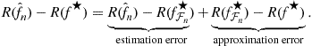
This decomposition is useful as the estimation error is the only random part. The approximation error depends on how rich the function class ![]() is but does not depend on the sample. The reason we have to trade these two errors off is that the richer the function class
is but does not depend on the sample. The reason we have to trade these two errors off is that the richer the function class ![]() the smaller the approximation error will be. However, that leads to a large estimation error. This trade-off is also known as the bias-variance trade-off. The bias-variance terminology comes from the regression with squared error case but tends to be used in the general loss setting as well.
the smaller the approximation error will be. However, that leads to a large estimation error. This trade-off is also known as the bias-variance trade-off. The bias-variance terminology comes from the regression with squared error case but tends to be used in the general loss setting as well.
1.14.2.3 Learnability with respect to a fixed class
Unlike universal consistency, which requires convergence to the minimum possible risk over all functions, learnability with respect to a fixed function class ![]() only demands that
only demands that
![]()
We can additionally require quantitative bounds on the number of samples needed to reach, with high probability, a given upper bound on excess risk relative to ![]() . The sample complexity of a learning rule
. The sample complexity of a learning rule ![]() is the minimum number
is the minimum number ![]() such that for all
such that for all ![]() , we have
, we have
![]()
with probability at least ![]() . We now see how we can arrive at sample complexity bounds for ERM via uniform convergence of empirical means to true expectations.
. We now see how we can arrive at sample complexity bounds for ERM via uniform convergence of empirical means to true expectations.
We mention some examples of functions classes that arise often in practice.
Linear Functions: This is one of the simplest functions classes. In any finite dimensional Euclidean space ![]() , define the class of real valued functions
, define the class of real valued functions
![]()
where ![]() denotes the standard inner product. The weight vector might be additionally constrained. For instance, we may require
denotes the standard inner product. The weight vector might be additionally constrained. For instance, we may require ![]() for some norm
for some norm ![]() . The set
. The set ![]() takes care of such constraints.
takes care of such constraints.
Linear Threshold Functions or Halfspaces: This is class of binary valued function obtained by thresholding linear functions at zero. This gives us the class
![]()
Reproducing Kernel Hilbert Spaces: Linear functions can be quite restricted in their approximation ability. However, we can get a significant improvement by first mapping the inputs ![]() into a feature space through a feature mapping
into a feature space through a feature mapping![]() where
where ![]() is a very high dimensional Euclidean space (or an infinite dimensional Hilbert space) and then considering linear functions in the feature space:
is a very high dimensional Euclidean space (or an infinite dimensional Hilbert space) and then considering linear functions in the feature space:
![]()
where the inner product now carries the subscript ![]() to emphasize the space where it operates. Many algorithms access the inputs only through pairwise inner products
to emphasize the space where it operates. Many algorithms access the inputs only through pairwise inner products
![]()
In such cases, we do not care what the feature mapping is or how complicated it is to evaluate, provided we can compute these inner products efficiently.
This idea of using only inner products leads us to reproducing kernel Hilbert space. We say that a function ![]() is symmetric positive semidefinite (psd) if it satisfies the following two properties.
is symmetric positive semidefinite (psd) if it satisfies the following two properties.
Positive Semidefiniteness: For any ![]() , the symmetric matrix
, the symmetric matrix
![]()
is psd.4 The matrix K is often called the Gram matrix.
Note that, given a feature mapping ![]() , it is trivial to verify that
, it is trivial to verify that
![]()
is a symmetric psd function. However, the much less trivial converse is also true. Every symmetric psd function arises out of a feature mapping. This is a consequence of the Moore-Aronszajn theorem. To state the theorem, we first need a definition. A reproducing kernel Hilbert space or RKHS![]() is a Hilbert space of functions
is a Hilbert space of functions ![]() such that there exists a kernel
such that there exists a kernel ![]() satisfying the properties:
satisfying the properties:
Theorem 3
Moore-Aronszajn
Given a symmetric psd function![]() , there is a unique RKHS
, there is a unique RKHS![]() with reproducing kernel K.
with reproducing kernel K.
This theorem gives us the feature mapping easily. Starting from a symmetric psd function K, we use the Moore-Aronszajn theorem to get an RKHS ![]() whose reproducing kernel is K. Now, by the reproducing property, for any
whose reproducing kernel is K. Now, by the reproducing property, for any ![]() ,
,
![]()
which means that ![]() given by
given by ![]() is a feature mapping we were looking for. Given this equivalence between symmetric psd functions and RKHSes, we will use the word kernel for a symmetric psd function itself.
is a feature mapping we were looking for. Given this equivalence between symmetric psd functions and RKHSes, we will use the word kernel for a symmetric psd function itself.
Convex Hulls: This example is not about a function class but rather about a means of obtaining a new function class from an old one. Say, we have class ![]() of binary valued functions
of binary valued functions ![]() . We can consider functions that take a majority vote over a subset of functions in
. We can consider functions that take a majority vote over a subset of functions in ![]() . That is,
. That is,

More generally, we can assign weights ![]() to
to ![]() and consider a weighted majority
and consider a weighted majority

Constraining the weights to sum to no more than W gives us the scaled convex hull
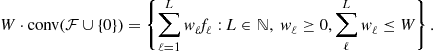
The class above can, of course, be thresholded to produce binary valued functions.
1.14.2.4 ERM and uniform convergence
The excess risk of ERM relative to ![]() can be decomposed as
can be decomposed as
![]()
By the definition of ERM, the difference ![]() is non-positive. The difference
is non-positive. The difference ![]() is also easy to deal with since it deals with a fixed (i.e. non-random) function
is also easy to deal with since it deals with a fixed (i.e. non-random) function ![]() . Using Hoeffding’s inequality (see Section 1.14.3.1), we have, with probability at least
. Using Hoeffding’s inequality (see Section 1.14.3.1), we have, with probability at least ![]() ,
,
![]()
This simply reflects the fact that as the sample size n grows, we expect the empirical average of ![]() to converge to its true expectation.
to converge to its true expectation.
The matter with the difference ![]() is not so simple since
is not so simple since ![]() is a random function. But we do know
is a random function. But we do know ![]() lies in
lies in ![]() . So we can clearly bound
. So we can clearly bound
![]() (14.1)
(14.1)
This provides a generalization bound (or, more properly, a generalization error bound) for ERM. A generalization bound is an upper bound on the true expectation ![]() of a learning rule in terms of its empirical performance
of a learning rule in terms of its empirical performance ![]() (or some other performance measure computed from data). A generalization bound typically involves additional terms that measure the statistical complexity of the class of functions that the learning rule uses. Note the important fact that the bound above is valid not just for ERM but for any learning rule that outputs a function
(or some other performance measure computed from data). A generalization bound typically involves additional terms that measure the statistical complexity of the class of functions that the learning rule uses. Note the important fact that the bound above is valid not just for ERM but for any learning rule that outputs a function ![]() .
.
The measure of complexity in the bound (14.1) above is the maximum deviation between true expectation and empirical average over functions in ![]() . For each fixed
. For each fixed![]() , we clearly have
, we clearly have
![]()
both in probability (weak law of large numbers) and almost surely (strong law of large numbers). But in order for
![]()
the law of large numbers has to hold uniformly over the function class ![]() .
.
To summarize, we have shown in this section that, with probability at least ![]() ,
,
![]() (14.2)
(14.2)
Thus, we can bound the excess risk of ERM if we can prove uniform convergence of empirical means to true expectations for the function class ![]() . This excess risk bound, unlike the generalization error bound (14.1), is applicable only to ERM.
. This excess risk bound, unlike the generalization error bound (14.1), is applicable only to ERM.
1.14.2.5 Bibliographic note
There are several book length treatments of learning theory that emphasize different aspects of the subject. The reader may wish to consult Anthony and Biggs [12], Anthony and Bartlett [13], Devroye et al. [14], Vapnik [15], Vapnik [6], Vapnik [16], Vidyasagar [17], Natarajan [18], Cucker and Zhou [19], Kearns and Vazirani [20], Cesa-Bianchi and Lugosi [21], Györfi et al. [22], and Hastie et al. [23].
1.14.3 Uniform convergence of empirical means
Let us consider the simplest case of a finite function class ![]() . In this case, Hoeffding’s inequality (see Theorem 5) gives us for any
. In this case, Hoeffding’s inequality (see Theorem 5) gives us for any ![]() , with probability at least
, with probability at least ![]() ,
,
![]()
Therefore, denoting the event that the above inequality fails to hold for function f by ![]() , we have
, we have
![]()
The first inequality is called a union bound in probability theory. It is exact if and only if all the events it is applied to are pairwise disjoint, i.e., ![]() for
for ![]() . Clearly, if there are functions that are “similar” to each other, the bound above will be loose. Nevertheless, the union bound is an important starting point for the analysis of uniform convergence of empirical means and for a finite class, it gives us the following result.
. Clearly, if there are functions that are “similar” to each other, the bound above will be loose. Nevertheless, the union bound is an important starting point for the analysis of uniform convergence of empirical means and for a finite class, it gives us the following result.
Theorem 4
Consider a finite class![]() and a loss function bounded by 1. Then, we have, with probability at least
and a loss function bounded by 1. Then, we have, with probability at least![]() ,
,
![]()
Therefore, using(14.2), we have the following result for ERM. With probability at least![]() ,
,
![]()
It is instructive to focus on the first term on the right hand side. First, it decreases as n increases. This means that ERM gets better as it works with more data. Second, it increases as the function class ![]() grows in size. But the dependence is logarithmic and hence mild.
grows in size. But the dependence is logarithmic and hence mild.
However, the bound above is useless if ![]() is not finite. The goal of the theory we will build below (often called “VC theory” after its architects Vapnik and Chervonenkis) will be to replace
is not finite. The goal of the theory we will build below (often called “VC theory” after its architects Vapnik and Chervonenkis) will be to replace ![]() with an appropriate measure of the capacity of an infinite function class
with an appropriate measure of the capacity of an infinite function class ![]() .
.
1.14.3.1 Concentration inequalities
Learning theory uses concentration inequalities heavily. A typical concentration inequality will state that a certain random variable is tightly concentrated around its mean (or in some cases median). That is, the probability that they deviate far enough from the mean is small.
The following concentration inequality, called Hoeffding’s inequality, applies to sums of iid random variables.
Theorem 5
Let![]() be bounded iid random variables with common expectation
be bounded iid random variables with common expectation![]() . Then we have, for
. Then we have, for![]()
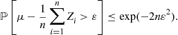
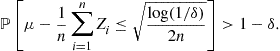
This can be restated as follows. For any![]() ,
,
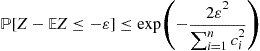
A couple of remarks are in order. First, even though we have stated Hoeffding’s inequality as applying to bounded iid random variables, only the boundedness and independence are really needed. It is possible to let the ![]() ’s have different distributions. Second, the above result provides probability upper bounds for deviations below the mean
’s have different distributions. Second, the above result provides probability upper bounds for deviations below the mean ![]() but a similar result holds for deviations of
but a similar result holds for deviations of ![]() above
above ![]() as well.
as well.
In fact, Hoeffding’s inequality can be considered a special case of the following inequality that is often called McDiarmid’s inequality or the bounded differences inequality.
Theorem 6
Let![]() be a function that satisfies the bounded differences property: for all
be a function that satisfies the bounded differences property: for all![]() and
and![]() ,
,
![]()
for some constants![]() . Then, for any independent
. Then, for any independent![]() , the random variable
, the random variable![]() satisfies,
satisfies,

as well as
for any![]() .
.
1.14.3.2 Rademacher complexity
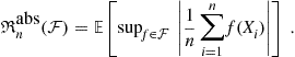
Let us recall that we need to control the following quantity:
![]()
Since this satisfies the conditions of McDiarmid’s inequality with ![]() , we have, with probability at least
, we have, with probability at least ![]() ,
,
![]()
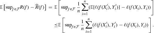
Now, we can appeal to a powerful idea known as symmetrization. The basic idea is to replace
![]()
with
![]()
where ![]() are samples drawn from the distribution P that are independent of each other and of the original sample. The new sample is often referred to as the ghost sample. The point of introducing the ghost sample is that, by an application of Jensen’s inequality, we get
are samples drawn from the distribution P that are independent of each other and of the original sample. The new sample is often referred to as the ghost sample. The point of introducing the ghost sample is that, by an application of Jensen’s inequality, we get
Now, the distribution of
![]()
is invariant under exchanging any ![]() with an
with an ![]() . That is, for any fixed choice of
. That is, for any fixed choice of ![]() signs
signs ![]() , the above quantity has the same distribution as
, the above quantity has the same distribution as
![]()
This allows us introduce even more randomization by making the ![]() ’s themselves random. This gives,
’s themselves random. This gives,

This directly yields a bound in terms of the Rademacher complexity:
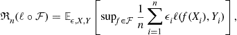
where ![]() is a Rademacher random variable that is either -1 or +1, each with probability
is a Rademacher random variable that is either -1 or +1, each with probability ![]() . The subscript below the expectation serves as a reminder that the expectation is being taken with respect to the randomness in
. The subscript below the expectation serves as a reminder that the expectation is being taken with respect to the randomness in ![]() ’s, and
’s, and ![]() ’s. We have thus proved the following theorem.
’s. We have thus proved the following theorem.
Theorem 7
Symmetrization
For a function class![]() and loss
and loss![]() , define the loss class
, define the loss class
![]()
We have,
![]()
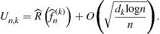
An interesting observation is that the sample dependent quantity
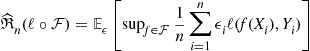
also satisfies the bounded differences condition with ![]() . This is the empirical Rademacher average and the expectation in its definition is only over the Rademacher random variables. Applying McDiarmid’s inequality, we have,
. This is the empirical Rademacher average and the expectation in its definition is only over the Rademacher random variables. Applying McDiarmid’s inequality, we have,
![]()
with probability at least ![]() .
.
To prove a bound on the Rademacher complexity of a finite class, the following lemma, due to [24], is useful.
Lemma 8
Massart’s finite class lemma
Let![]() be a finite subset of
be a finite subset of![]() and
and![]() be independent Rademacher random variables. Let
be independent Rademacher random variables. Let![]() . Then, we have,
. Then, we have,

Therefore, for any finite class![]() consisting of functions bounded by 1,
consisting of functions bounded by 1,
![]()
Since the right hand side is not random, the same bound holds for![]() as well.
as well.
The Rademacher complexity, and its empirical counterpart, satisfy a number of interesting structural properties.
Theorem 9
Structural Properties of Rademacher Complexity
Let![]() and
and![]() be classes of real valued functions. Then
be classes of real valued functions. Then![]() (as well as
(as well as![]() ) satisfies the following properties:
) satisfies the following properties:
For proofs of these properties, see [25]. However, note that the Rademacher complexity is defined there such that an extra absolute value is taken before the supremum over ![]() . That is,
. That is,
Nevertheless, the proofs given there generalize quite easily to definition of Rademacher complexity that we are using. For example, see [26], where the Rademacher complexity as we have defined it here (without the absolute value) is called free Rademacher complexity.
Using these properties, it is possible to directly bound the Rademacher complexity of several interesting functions classes. See [25] for examples. The contraction property is a very useful one. It allows us to transition from the Rademacher complexity of the loss class to the Rademacher complexity of the function class itself (for Lipschitz losses).
The Rademacher complexity can also be bounded in terms of another measure of complexity of a function class: namely covering numbers.
1.14.3.3 Covering numbers
The idea underlying covering numbers is very intuitive. Let ![]() be any (pseudo-) metric space and fix a subset
be any (pseudo-) metric space and fix a subset ![]() . A set
. A set ![]() is said to be an
is said to be an ![]() -cover of T if
-cover of T if
![]()
In other words “balls” of radius ![]() placed at elements of
placed at elements of ![]() “cover” the set T entirely. The covering number (at scale
“cover” the set T entirely. The covering number (at scale ![]() ) of T is defined as the size of the smallest cover of T (at scale
) of T is defined as the size of the smallest cover of T (at scale ![]() ).
).
![]()
The logarithm of covering number is called entropy.
Given a sample ![]() , define the data dependent metric on
, define the data dependent metric on ![]() as
as
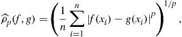
where ![]() . Taking the limit
. Taking the limit ![]() suggests the metric
suggests the metric
![]()
These metrics gives us the p-norm covering numbers
![]()
These covering numbers increase with p. That is, for ![]() ,
,
![]()
Finally, we can also define the worst case (over samples) p-norm covering number
![]()
A major result connecting Rademacher complexity with covering numbers is due to [27].
Theorem 10
Dudley’s entropy integral bound
For any![]() consisting of real valued functions bounded by 1, we have
consisting of real valued functions bounded by 1, we have
![]()
Therefore, using Jensen’s inequality, we have
![]()
1.14.3.4 Binary valued functions: VC dimension
For binary function classes ![]() , we can provide distribution free upper bounds on the Rademacher complexity or covering numbers in terms of a combinatorial parameter called the Vapnik-Chervonenkis (VC) dimension.
, we can provide distribution free upper bounds on the Rademacher complexity or covering numbers in terms of a combinatorial parameter called the Vapnik-Chervonenkis (VC) dimension.
To define it, consider a sequence ![]() . We say that
. We say that ![]() is shattered by
is shattered by ![]() if each of the
if each of the ![]() possible
possible ![]() labelings of these n points are realizable using some
labelings of these n points are realizable using some ![]() . That is,
. That is, ![]() is shattered by
is shattered by ![]() iff
iff
![]()
The VC dimension of ![]() is the length of the longest sequence that can shattered by
is the length of the longest sequence that can shattered by ![]() :
:
![]()
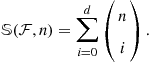
The size of the restriction of ![]() to
to ![]() is called the shatter coefficient:
is called the shatter coefficient:
![]()
Considering the worst sequence gives us the growth function
![]()
If ![]() , then we know that
, then we know that ![]() for all
for all ![]() . One can ask: what is the behavior of the growth function for
. One can ask: what is the behavior of the growth function for ![]() ? The following combinatorial lemma proved independently by Vapnik and Chervonenkis [28], Sauer [29], and Shelah [30], gives the answer to this question.
? The following combinatorial lemma proved independently by Vapnik and Chervonenkis [28], Sauer [29], and Shelah [30], gives the answer to this question.
Lemma 11
If ![]() , then we have, for any
, then we have, for any![]() ,
,
In particular, if![]() .
.
Thus, for a class with finite VC dimension, the Rademacher complexity can be bounded directly using Massart’s lemma.
Theorem 12
Suppose![]() . Then, we have,
. Then, we have,
![]()
It is possible to shave off the ![]() factor in the bound above plugging an estimate of the entropy
factor in the bound above plugging an estimate of the entropy ![]() for VC classes due to [31] into Theorem 10.
for VC classes due to [31] into Theorem 10.
Theorem 13
Suppose![]() . We have, for any
. We have, for any![]() ,
,
![]()
for a universal constant C.
These results show that for a class ![]() with finite VC dimension d, the sample complexity required by ERM to achieve
with finite VC dimension d, the sample complexity required by ERM to achieve ![]() excess risk relative to
excess risk relative to ![]() is, with probability at least
is, with probability at least ![]() . Therefore, a finite VC dimension is sufficient for learnability with respect to a fixed functions class. In fact, a finite VC dimension also turns out to be necessary (see, for instance, [14, Chapter 14]). Thus, we have the following characterization.
. Therefore, a finite VC dimension is sufficient for learnability with respect to a fixed functions class. In fact, a finite VC dimension also turns out to be necessary (see, for instance, [14, Chapter 14]). Thus, we have the following characterization.
Theorem 14
In the binary classification setting with 0–1 loss, there is a learning algorithm with bounded sample complexity for every![]() iff
iff![]() .
.
Note that, when ![]() , the dependence of the sample complexity on
, the dependence of the sample complexity on ![]() is polynomial and on
is polynomial and on ![]() is logarithmic. Moreover, such a sample complexity is achieved by ERM. On the other hand, when
is logarithmic. Moreover, such a sample complexity is achieved by ERM. On the other hand, when ![]() , then no learning algorithm, including ERM, can have bounded sample complexity for arbitrarily small
, then no learning algorithm, including ERM, can have bounded sample complexity for arbitrarily small ![]() .
.
1.14.3.5 Real valued functions: fat shattering dimension
For real valued functions, getting distribution free upper bounds on Rademacher complexity or covering numbers involves combinatorial parameters similar to the VC dimension. The appropriate notion for determining learnability using a finite number of samples turns out to be a scale sensitive combinatorial dimension known as the fat shattering dimension.
Fix a class ![]() consisting of bounded real valued functions
consisting of bounded real valued functions ![]() and a scale
and a scale ![]() . We say that a sequence
. We say that a sequence ![]() is
is ![]() -shattered by
-shattered by ![]() if there exists a witness sequence
if there exists a witness sequence ![]() such that, for every
such that, for every ![]() , there is an
, there is an ![]() such that
such that
![]()
In words, this means that, for any of the ![]() possibilities for the sign pattern
possibilities for the sign pattern ![]() , we have a function
, we have a function ![]() whose values at the points
whose values at the points ![]() is above or below
is above or below ![]() depending on whether
depending on whether ![]() is
is ![]() or
or ![]() . Moreover, the gap between
. Moreover, the gap between ![]() and
and ![]() is required to be at least
is required to be at least ![]() .
.
The fat-shattering dimension of ![]() at scale
at scale ![]() is the size of the longest sequence that can be
is the size of the longest sequence that can be ![]() -shattered by
-shattered by ![]() :
:
![]()
A bound on ![]() -norm covering numbers in terms of the fat shattering dimension were first given by Alon et al. [32].
-norm covering numbers in terms of the fat shattering dimension were first given by Alon et al. [32].
Theorem 15
Fix a class![]() . Then we have, for any
. Then we have, for any![]() ,
,
![]()
where![]() .
.
Using this bound, the sample complexity of learning a real valued function class of bounded range using a Lipschitz loss5![]() is
is ![]() where
where ![]() for a universal constant
for a universal constant ![]() . The importance of the fat shattering dimension lies in the fact that if
. The importance of the fat shattering dimension lies in the fact that if ![]() for some
for some ![]() , then no learning algorithm can have bounded sample complexity for learning the functions for arbitrarily small values of
, then no learning algorithm can have bounded sample complexity for learning the functions for arbitrarily small values of ![]() .
.
Theorem 16
In the regression setting with either squared loss or absolute loss, there is a learning algorithm with bounded sample complexity for every![]() iff
iff![]() .
.
Note that here, unlike the binary classification case, the dependence of the sample complexity on ![]() is not fixed. It depends on how fast
is not fixed. It depends on how fast ![]() grows as
grows as ![]() . In particular, if
. In particular, if ![]() grows as
grows as ![]() then the sample complexity is polynomial in
then the sample complexity is polynomial in ![]() (and logarithmic in
(and logarithmic in ![]() ).
).
1.14.4 Model selection
In general, model selection refers to the task of selecting an appropriate model from a given family based on available data. For ERM, the “model” is the class ![]() of functions
of functions ![]() that are intended to capture the functional dependence between the input variable X and the output Y. If we choose too small an
that are intended to capture the functional dependence between the input variable X and the output Y. If we choose too small an ![]() then ERM will not have good performance if
then ERM will not have good performance if ![]() is not even well approximated by any member of
is not even well approximated by any member of ![]() . One the other hand, if
. One the other hand, if ![]() is too large (say all functions) then the estimation error will be so large that ERM will not perform well even if
is too large (say all functions) then the estimation error will be so large that ERM will not perform well even if ![]() .
.
1.14.4.1 Structural risk minimization
Consider the classification setting with 0–1 loss. Suppose we have a countable sequence of nested function classes:
![]()
where ![]() has VC dimension
has VC dimension ![]() . The function
. The function ![]() chosen by ERM over
chosen by ERM over ![]() satisfies the bound
satisfies the bound
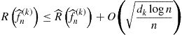
with high probability. As k increases, the classes become more complex. So, the empirical risk term will decrease with k whereas the VC dimension term will increase. The principle of structural risk minimization (SRM) chooses a value of k by minimizing the right hand side above.
Namely, we choose
![]() (14.3)
(14.3)
for some universal constant C.
It can be shown (see, for example, [14, Chapter 18]) that SRM leads to universally consistent rules provided appropriate conditions are placed on the functions classes ![]() .
.
Theorem 17
Universal Consistency of SRM
Let![]() be a sequence of classes such that for any distribution P,
be a sequence of classes such that for any distribution P,
![]()
Assume also that![]() are all finite. Then the learning rule
are all finite. Then the learning rule![]() with
with![]() chosen as in(14.3)is strongly universally consistent.
chosen as in(14.3)is strongly universally consistent.
The penalty term in (14.3) depends on the VC dimension of ![]() . It turns out that it is not essential. All we need is an upper bound on the risk of ERM in terms of the empirical risk and some measure of the complexity of the function class. One could also imagine proving results for regression problems by replacing the VC dimension with fat-shattering dimension. We can think of SRM as penalizing larger classes by their capacity to overfit the data. However, the penalty in SRM is fixed in advance and is not data dependent. We will now look into more general penalties.
. It turns out that it is not essential. All we need is an upper bound on the risk of ERM in terms of the empirical risk and some measure of the complexity of the function class. One could also imagine proving results for regression problems by replacing the VC dimension with fat-shattering dimension. We can think of SRM as penalizing larger classes by their capacity to overfit the data. However, the penalty in SRM is fixed in advance and is not data dependent. We will now look into more general penalties.
1.14.4.2 Model selection via penalization
Given a (not necessarily nested) countable or finite collection of models ![]() and a penalty function
and a penalty function ![]() , define
, define ![]() as the minimizer of
as the minimizer of
![]()
Recall that ![]() is the result of ERM over
is the result of ERM over ![]() . Also note that the penalty can additionally depend on the data. Now define the penalized estimator as
. Also note that the penalty can additionally depend on the data. Now define the penalized estimator as
![]()
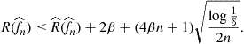
The following theorem shows that any probabilistic upper bound ![]() on the risk
on the risk ![]() can be used to design a penalty for which a performance bound can be given.
can be used to design a penalty for which a performance bound can be given.
Theorem 18
Assume that there are positive numbers c and m such that for each k we have the guarantee
![]()
Then the penalized estimator![]() with
with
![]()
satisfies
![]()
Note that the result says that the penalized estimator achieves an almost optimal trade-off between the approximation error ![]() and the expected complexity
and the expected complexity ![]() . For a good upper bound
. For a good upper bound ![]() , the expected complexity will be a good upper bound on the (expected) estimation error. Therefore, the model selection properties of the penalized estimator depend on how good an upper bound
, the expected complexity will be a good upper bound on the (expected) estimation error. Therefore, the model selection properties of the penalized estimator depend on how good an upper bound ![]() we can find.
we can find.
Note that structural risk minimization corresponds to using a distribution free upper bound
The looseness of these distribution free upper bounds has prompted researchers to design data dependent penalties. We shall see an examples based on empirical Rademacher averages in the next section.
Proof
For any ![]() ,
,
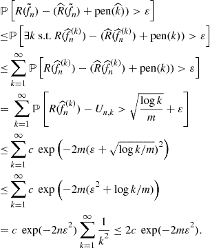
By integrating the final upper bound with respect to ![]() , we get the bound
, we get the bound
![]() (14.4)
(14.4)
Also, for any k, we have

The first inequality above follows by definition of ![]() and
and ![]() . The second holds because
. The second holds because ![]() minimizes the empirical risk over
minimizes the empirical risk over ![]() . Summing this with (14.4), we get, for any k,
. Summing this with (14.4), we get, for any k,
![]()
Now subtracting ![]() from both sides and minimizing over k proves the theorem.
from both sides and minimizing over k proves the theorem. ![]()
1.14.4.3 Data driven penalties using Rademacher averages
The results of Section 1.14.3.2 tell us that there exists universal constants ![]() such that
such that
![]()
Thus, we can use the data dependent penalty
![]()
in Theorem 18 to get the bound

Note that the penalty here is data dependent. Moreover, except for the ![]() term, the penalized estimator makes the optimal trade-off between the Rademacher complexity, an upper bound on the estimation error, and the approximation error.
term, the penalized estimator makes the optimal trade-off between the Rademacher complexity, an upper bound on the estimation error, and the approximation error.
1.14.4.4 Hold-out estimates
Suppose out of ![]() iid samples we set aside m samples where m is much smaller than n. Since the hold-out set of size m is not used in the computation of
iid samples we set aside m samples where m is much smaller than n. Since the hold-out set of size m is not used in the computation of ![]() , we can estimate
, we can estimate ![]() by the hold-out estimate
by the hold-out estimate
![]()
By Hoeffding’s inequality, the assumption of Theorem 18 holds with ![]() . Moreover
. Moreover ![]() . Therefore, we have
. Therefore, we have

1.14.5 Alternatives to uniform convergence
The approach of deriving generalization bounds using uniform convergence arguments is not the only one possible. In this section, we review three techniques for proving generalization bounds based on sample compression, algorithmic stability, and PAC-Bayesian analysis respectively.
1.14.5.1 Sample compression
The sample compression approach to proving generalization bounds was introduced by [33]. It applies to algorithms whose output ![]() (that is learned using some training set S) can be reconstructed from a compressed subset
(that is learned using some training set S) can be reconstructed from a compressed subset ![]() . Here
. Here ![]() is a sequence of indices
is a sequence of indices
![]()
and ![]() is simply the subsequence of S indexed by
is simply the subsequence of S indexed by ![]() . For the index sequence
. For the index sequence ![]() above, we say that its length
above, we say that its length ![]() is k. To formalize the idea that the algorithms output can be reconstructed from a small number of examples, we will define a compression function
is k. To formalize the idea that the algorithms output can be reconstructed from a small number of examples, we will define a compression function
![]()
where ![]() is the set of all possible index sequences of finite length. It is assumed that
is the set of all possible index sequences of finite length. It is assumed that ![]() for an S is of size n. We also define a reconstruction function
for an S is of size n. We also define a reconstruction function
![]()
We assume that the learning rule satisfies, for any S,
![]() (14.5)
(14.5)
This formalizes our intuition that to reconstruct ![]() it suffices to remember only those examples whose indices are given by
it suffices to remember only those examples whose indices are given by ![]() .
.
The following result gives a generalization bound for such an algorithm.
Theorem 19
Let![]() be a learning rule for which there exists compression and reconstructions functions
be a learning rule for which there exists compression and reconstructions functions![]() and
and![]() respectively such that the equality(14.5)holds for all S. Then, we have, with probability at least
respectively such that the equality(14.5)holds for all S. Then, we have, with probability at least![]() ,
,

where![]() .
.
Proof
The proof uses the simple idea that for a fixed index set ![]() is a sample of size
is a sample of size ![]() that is independent of
that is independent of ![]() . Here
. Here ![]() denotes the sequence
denotes the sequence ![]() . By this independence, the risk of any function that depends only on
. By this independence, the risk of any function that depends only on ![]() is close to its empirical average on
is close to its empirical average on ![]() by Hoeffding’s inequality.
by Hoeffding’s inequality.
Denote the empirical risk of f calculated on a subset ![]() of S by
of S by ![]() . We have, for any f,
. We have, for any f,
![]()
where ![]() . Thus, all we need to show is
. Thus, all we need to show is
![]()
where

To show this, we proceed as follows,
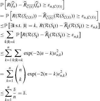
The last step holds because, by our choice of ![]() ,
,

1.14.5.2 Stability
Stability is property of a learning algorithm that ensures that the output, or some aspect of the output, of the learning algorithm does not change much if the training data set changes very slightly. This is an intuitive notion whose roots in learning theory go back to the work of Tikhonov on regularization of inverse problems. To see how stability can be used to give generalization bounds, let us consider a result of Bousquet and Elisseeff [34] that avoids going through uniform convergence arguments by directly showing that any learning algorithm with uniform stability enjoys exponential tail generalization bounds in terms of both the training error and the leave-one-out error of the algorithm.
Let ![]() denote the sample of size
denote the sample of size ![]() obtained by removing a particular input
obtained by removing a particular input ![]() from a sample S of size n. A learning algorithm is said to have uniform stability
from a sample S of size n. A learning algorithm is said to have uniform stability![]() if for any
if for any ![]() and any
and any ![]() , we have,
, we have,
![]()
We have the following generalization bound for a uniformly stable learning algorithm.
Theorem 20
Let![]() have uniform stability
have uniform stability![]() . Then, with probability at least
. Then, with probability at least![]() ,
,
Note that this theorem gives tight bound when ![]() scales as
scales as ![]() . As such it cannot be applied directly to the classification setting with 0–1 loss where
. As such it cannot be applied directly to the classification setting with 0–1 loss where ![]() can only be 0 or 1. A good example of a learning algorithm that exhibits uniform stability is regularized ERM over a reproducing kernel Hilbert space using a convex loss function that has Lipschitz constant
can only be 0 or 1. A good example of a learning algorithm that exhibits uniform stability is regularized ERM over a reproducing kernel Hilbert space using a convex loss function that has Lipschitz constant ![]() :
:
![]()
A regularized ERM using kernel K is defined by
![]()
where ![]() is a regularization parameter. Regularized ERM has uniform stability
is a regularization parameter. Regularized ERM has uniform stability ![]() for
for ![]() , where
, where
![]()
The literature on stability of learning algorithms is unfortunately thick with definitions. For instance, Kutin and Niyogi [35] alone consider over a dozen variants! We chose a simple (but quite strong) definition from Bousquet and Elisseeff above to illustrate the general point that stability can be used to derive generalization bounds. But we like to point the reader to Mukherjee et al. [36] where a notion of leave-one-out (LOO) stability is defined and shown sufficient for generalization for any learning algorithm. Moreover, for ERM they show it is necessary and sufficient for both generalization and learnability with respect to a fixed class. Shalev-Shwartz et al. [37] further examine the connections between stability, generalization and learnability in Vapnik’s general learning setting that includes supervised learning (learning from example, label pairs) as a special case.
1.14.5.3 PAC-Bayesian analysis
PAC-Bayesian analysis refers to a style of analysis of learning algorithms that output not just a single function ![]() but rather a distribution (called a “posterior distribution”) over
but rather a distribution (called a “posterior distribution”) over ![]() . Moreover, the complexity of the data-dependent posterior distribution is measured relative to a fixed distribution chosen in advance (that is, in a data independent way). The fixed distribution is called a “prior distribution.” Note that the terms “prior” and “posterior” are borrowed from the analysis of Bayesian algorithms that start with a prior distribution on some parameter space and, on seeing data, make updates to the distribution using Bayes’ rule to obtain a posterior distribution. Even though the terms are borrowed, their use is not required to be similar to their use in Bayesian analysis. In particular, the prior used in the PAC-Bayes theorem need not be “true” in any sense and the posterior need not be obtained using Bayesian updates: the bound holds for any choice of the prior and posterior.
. Moreover, the complexity of the data-dependent posterior distribution is measured relative to a fixed distribution chosen in advance (that is, in a data independent way). The fixed distribution is called a “prior distribution.” Note that the terms “prior” and “posterior” are borrowed from the analysis of Bayesian algorithms that start with a prior distribution on some parameter space and, on seeing data, make updates to the distribution using Bayes’ rule to obtain a posterior distribution. Even though the terms are borrowed, their use is not required to be similar to their use in Bayesian analysis. In particular, the prior used in the PAC-Bayes theorem need not be “true” in any sense and the posterior need not be obtained using Bayesian updates: the bound holds for any choice of the prior and posterior.
Denote the space of probability distributions over ![]() by
by ![]() . There might be measurability issues in defining this for general function classes. So, we can assume that
. There might be measurability issues in defining this for general function classes. So, we can assume that ![]() is a countable class for the purpose of the theorem below. Note, however, that the cardinality of the class
is a countable class for the purpose of the theorem below. Note, however, that the cardinality of the class ![]() never enters the bound explicitly anywhere. For any
never enters the bound explicitly anywhere. For any ![]() , define
, define
![]()
In the context of classification, a randomized classifier that, when asked for a prediction, samples a function from a distribution ![]() and uses if for classification, is called a Gibbs classifier. Note that
and uses if for classification, is called a Gibbs classifier. Note that ![]() is the risk of such a Gibbs classifier.
is the risk of such a Gibbs classifier.
Also recall the definition of Kullback-Leibler divergence or relative entropy:
![]()
For real numbers ![]() we define (with some abuse of notation):
we define (with some abuse of notation):
![]()
With these definitions, we can now state the PAC Bayesian theorem [38].
Theorem 21
PAC-Bayesian Theorem
Let![]() be a fixed distribution over
be a fixed distribution over![]() . Then, we have, with probability at least
. Then, we have, with probability at least![]() ,
,
![]()
In particular, for any learning algorithm that, instead of returning a single function![]() , returns a distribution
, returns a distribution![]() over
over![]() , we have, with probability at least
, we have, with probability at least![]() ,
,
![]()
To get more interpretable bounds from this statement, the following inequality is useful for ![]() :
:
![]()
This implies that if ![]() then two inequalities hold:
then two inequalities hold:
![]()
The first gives us a version of the PAC-Bayesian bound that is often presented:

The second gives us the interesting bound

If the loss ![]() is close to zero, then the dominating term is the second term that scales as
is close to zero, then the dominating term is the second term that scales as ![]() . If not, then the first term, which scales as
. If not, then the first term, which scales as ![]() , dominates.
, dominates.
1.14.6 Computational aspects
So far we have only talked about sample complexity issues ignoring considerations of computational complexity. To properly address the latter, we need a formal model of computation and need to talk about how functions are represented by the learning algorithm. The branch of machine learning that studies these questions is called computational learning theory. We will now provide a brief introduction to this area.
1.14.6.1 The PAC model
The basic model in computational learning theory is the Probably Approximately Correct (PAC) model. It applies to learning binary valued functions and uses the 0–1 loss. Since a ![]() valued function is specified unambiguously be specifying the subset of
valued function is specified unambiguously be specifying the subset of ![]() where it is one, we have a bijection between binary valued functions and concepts, which are simply subsets of
where it is one, we have a bijection between binary valued functions and concepts, which are simply subsets of ![]() . Thus we will use (binary valued) function and concept interchangeably in this section. Moreover, the basic PAC model considers what is sometimes called the realizable case. That is, there is a “true” concept in
. Thus we will use (binary valued) function and concept interchangeably in this section. Moreover, the basic PAC model considers what is sometimes called the realizable case. That is, there is a “true” concept in ![]() generating the data. This means that
generating the data. This means that ![]() for some
for some ![]() . Hence the minimal risk in the class is zero:
. Hence the minimal risk in the class is zero: ![]() . Note, however, that the distribution over
. Note, however, that the distribution over ![]() is still assumed to be arbitrary.
is still assumed to be arbitrary.
To define the computational complexity of a learning algorithm, we assume that ![]() is either
is either ![]() or
or ![]() . We assume a model of computation that can store a single real number in a memory location and can perform any basic arithmetic operation (additional, subtraction, multiplication, division) on two real numbers in one unit of computation time.
. We assume a model of computation that can store a single real number in a memory location and can perform any basic arithmetic operation (additional, subtraction, multiplication, division) on two real numbers in one unit of computation time.
The distinction between a concept and its representation is also an important one when we study computational complexity. For instance, if our concepts are convex polytopes in ![]() , we may choose a representation scheme that specifies the vertices of the polytope. Alternatively, we may choose to specify the linear equalities describing the faces of the polytope. Their vertex-based and face-based representations can differ exponentially in size. Formally, a representation scheme is a mapping
, we may choose a representation scheme that specifies the vertices of the polytope. Alternatively, we may choose to specify the linear equalities describing the faces of the polytope. Their vertex-based and face-based representations can differ exponentially in size. Formally, a representation scheme is a mapping ![]() that maps a representation (consisting of symbols from a finite alphabet
that maps a representation (consisting of symbols from a finite alphabet ![]() and real numbers) to a concept. As noted above, there could be many
and real numbers) to a concept. As noted above, there could be many ![]() ’s such that
’s such that ![]() for a given concept f. The size of representation is assumed to be given by a function
for a given concept f. The size of representation is assumed to be given by a function ![]() . A simple choice of size could be simply the number of symbols and real numbers that appear in the representation. Finally, the size of a concept f is simply the size of its smallest representation:
. A simple choice of size could be simply the number of symbols and real numbers that appear in the representation. Finally, the size of a concept f is simply the size of its smallest representation:
![]()
The last ingredient we need before can give the definition of efficient learnability in the PAC model is the representation class ![]() used by the algorithm for producing its output. We call
used by the algorithm for producing its output. We call ![]() the hypothesis class and it is assumed that there is a representation in
the hypothesis class and it is assumed that there is a representation in ![]() for every function in
for every function in ![]() . Moreover, it is required that for every
. Moreover, it is required that for every ![]() and any
and any ![]() , we can evaluate
, we can evaluate ![]()
![]() in time polynomial in d and size
in time polynomial in d and size![]() .
.
Recall that we have assumed ![]() or
or ![]() . We say that an algorithm efficiently PAC learns
. We say that an algorithm efficiently PAC learns![]() using hypothesis class
using hypothesis class ![]() if, for any
if, for any ![]() , given access to iid examples
, given access to iid examples ![]() , inputs
, inputs ![]() (accuracy),
(accuracy), ![]() (confidence), and
(confidence), and ![]() , the algorithm satisfies the following conditions:
, the algorithm satisfies the following conditions:
For examples of classes ![]() that are efficiently PAC learnable (using some
that are efficiently PAC learnable (using some ![]() ), see the texts [12,18,20].
), see the texts [12,18,20].
1.14.6.2 Weak and strong learning
In the PAC learning definition, the algorithm must be able to achieve arbitrarily small values of ![]() and
and ![]() . A weaker definition would require the learning algorithm to work only for fixed choices of
. A weaker definition would require the learning algorithm to work only for fixed choices of ![]() and
and ![]() . We can modify the definition of PAC learning by removing
. We can modify the definition of PAC learning by removing ![]() and
and ![]() from the input to the algorithm. Instead, we assume that there are fixed polynomials
from the input to the algorithm. Instead, we assume that there are fixed polynomials ![]() and
and ![]() such that the algorithm outputs
such that the algorithm outputs ![]() that satisfies
that satisfies
![]()
with probability at least
![]()
Such an algorithm is called a weak PAC learning algorithm for ![]() . The original definition, in contrast, can be called a definition of strong PAC learning. The definition of weak PAC learning does appear quite weak. Recall that an accuracy of
. The original definition, in contrast, can be called a definition of strong PAC learning. The definition of weak PAC learning does appear quite weak. Recall that an accuracy of ![]() can be trivially achieved by an algorithm that does not even look at the samples but simply outputs a hypothesis that outputs a random
can be trivially achieved by an algorithm that does not even look at the samples but simply outputs a hypothesis that outputs a random ![]() sign (each with probability a half) for any input. The desired accuracy above is just an inverse polynomial away from the trivial accuracy guarantee of
sign (each with probability a half) for any input. The desired accuracy above is just an inverse polynomial away from the trivial accuracy guarantee of ![]() . Moreover, the probability with which the weak accuracy is achieved is not required to be arbitrarily close to 1.
. Moreover, the probability with which the weak accuracy is achieved is not required to be arbitrarily close to 1.
A natural question to ask is whether a class that is weakly PAC learnable using ![]() is also strongly learnable using
is also strongly learnable using ![]() ? The answer, somewhat surprisingly, is “Yes.” So, the weak PAC learning definition only appears to be a relaxed version of strong PAC learning. Moreover, a weak PAC learning algorithm, given as a subroutine or blackbox, can be converted into a strong PAC learning algorithm. Such a conversion is called boosting.
? The answer, somewhat surprisingly, is “Yes.” So, the weak PAC learning definition only appears to be a relaxed version of strong PAC learning. Moreover, a weak PAC learning algorithm, given as a subroutine or blackbox, can be converted into a strong PAC learning algorithm. Such a conversion is called boosting.
A boosting procedure has to start with a weak learning algorithm and boost two things: the confidence and the accuracy. It turns out that boosting the confidence is easier. The basic idea is to run the weak learning algorithm several times on independent samples. Therefore, the crux of the boosting procedure lies in boosting the accuracy. Boosting the accuracy seems hard until one realizes that the weak learning algorithm does have one strong property: it is guaranteed to work no matter what the underlying distribution of the examples is. Thus, if a first run of the weak learning only produces a hypothesis ![]() with slightly better accuracy than
with slightly better accuracy than ![]() , we can make the second run focus only on those examples where
, we can make the second run focus only on those examples where ![]() makes a mistake. Thus, we will focus the weak learning algorithm on “harder portions” of the input distribution. While this simple idea does not directly work, a variation on the same theme was shown to work by Schapire [39]. Freund [40] then presented a simpler boosting algorithm. Finally, a much more practical boosting procedure, called AdaBoost, was discovered by them jointly [10]. AdaBoost counts as one of the great practical success stories of computational learning theory. For more details on boosting, AdaBoost, and the intriguing connections of these ideas to game theory and statistics, we refer the reader to [41].
makes a mistake. Thus, we will focus the weak learning algorithm on “harder portions” of the input distribution. While this simple idea does not directly work, a variation on the same theme was shown to work by Schapire [39]. Freund [40] then presented a simpler boosting algorithm. Finally, a much more practical boosting procedure, called AdaBoost, was discovered by them jointly [10]. AdaBoost counts as one of the great practical success stories of computational learning theory. For more details on boosting, AdaBoost, and the intriguing connections of these ideas to game theory and statistics, we refer the reader to [41].
1.14.6.3 Random classification noise and the SQ model
Recall that the basic PAC model assumes that the labels are generated using a function f belonging to the class ![]() under consideration. Our earlier development of statistical tools for obtaining sampling complexity estimates did not require such an assumptions (though the rates did depend on whether
under consideration. Our earlier development of statistical tools for obtaining sampling complexity estimates did not require such an assumptions (though the rates did depend on whether ![]() or not).
or not).
There are various noise models that extend the PAC model by relaxing the noise-free assumption and thus making the problem of learning potentially harder. Perhaps the simplest is the random classification noise model [42]. In this model, when the learning algorithm queries for the next labeled example of the form ![]() , it receives it with probability
, it receives it with probability ![]() but with probability
but with probability ![]() , it receives
, it receives ![]() . That is, with some probability
. That is, with some probability ![]() , the label is flipped. The definition of efficient learnability remains the same except that now the learning algorithm has to run in time polynomial in
, the label is flipped. The definition of efficient learnability remains the same except that now the learning algorithm has to run in time polynomial in ![]() and
and ![]() where
where ![]() is an input to the algorithm and is an upper bound on
is an input to the algorithm and is an upper bound on ![]() .
.
Kearns [43] introduced the statistical query (SQ) model where learning algorithms do not directly access the labeled example but only make statistical queries about the underlying distribution. The queries take the form ![]() where
where ![]() is a binary valued function of the labeled examples and
is a binary valued function of the labeled examples and ![]() is a tolerance parameter. Given such a query, the oracle in the SQ model responds with an estimate of
is a tolerance parameter. Given such a query, the oracle in the SQ model responds with an estimate of ![]() that is accurate to within an additive error of
that is accurate to within an additive error of ![]() . It is easy to see, using Hoeffding’s inequality, that given access to the usual PAC oracle that provides iid examples of the form
. It is easy to see, using Hoeffding’s inequality, that given access to the usual PAC oracle that provides iid examples of the form ![]() , we can simulate the SQ oracle by just drawing a sample of size polynomial in
, we can simulate the SQ oracle by just drawing a sample of size polynomial in ![]() and
and ![]() and estimating the probability
and estimating the probability ![]() based on it. The simulation with succeed with probability
based on it. The simulation with succeed with probability ![]() . Kearns gave a more complicated simulation that mimics the SQ oracle given access to only a PAC oracle with random misclassification noise.
. Kearns gave a more complicated simulation that mimics the SQ oracle given access to only a PAC oracle with random misclassification noise.
Lemma 22
Given a query![]() , the probability
, the probability![]() can be estimated to within
can be estimated to within![]() error, with probability at least
error, with probability at least![]() , using
, using

examples that have random misclassification noise at rate![]() in them.
in them.
This lemma means that learning algorithm that learns a concept class ![]() in the SQ model can also learn
in the SQ model can also learn ![]() in the random classification noise model.
in the random classification noise model.
Theorem 23
If there is an algorithm that efficiently learns![]() from statistical queries using
from statistical queries using![]() , then there is an algorithm that efficiently learns
, then there is an algorithm that efficiently learns![]() using
using![]() in the random classification noise model.
in the random classification noise model.
1.14.6.4 The agnostic PAC model
The agnostic PAC model uses the same definition of learning as the one we used in Section 1.14.2.3). That is, the distribution of examples ![]() is arbitrary. In particular, it is not assumed that
is arbitrary. In particular, it is not assumed that ![]() for any f. The goal of the learning algorithm is to output a hypothesis
for any f. The goal of the learning algorithm is to output a hypothesis ![]() with
with ![]() with probability at least
with probability at least ![]() . We say that a learning algorithm efficiently learns
. We say that a learning algorithm efficiently learns ![]() using
using ![]() in the agnostic PAC model if the algorithm not only outputs a probably approximately correct hypothesis h but also runs in time that is polynomial in
in the agnostic PAC model if the algorithm not only outputs a probably approximately correct hypothesis h but also runs in time that is polynomial in ![]() , and d.
, and d.
The agnostic model has proved to be a very difficult one for exhibiting efficient learning algorithms. Note that the statistical issue is completely resolved: a class ![]() is learnable iff it has finite VC dimension. However, the “algorithm” implicit in this statement is ERM which, even for the class of halfspaces
is learnable iff it has finite VC dimension. However, the “algorithm” implicit in this statement is ERM which, even for the class of halfspaces
![]()
leads to NP-hard problems. For instance, see [44] for very strong negative results about agnostic learning of halfspaces. However, these results apply to proper agnostic learning only. That is, the algorithm outputs a hypothesis that is also a halfspace. An efficient algorithm for learning halfspaces in the agnostic PAC model using a general hypothesis class would be a major breakthrough.
1.14.6.5 The mistake bound model
The mistake bound model is quite different from the PAC model. Unlike the PAC model, no assumption is made on the distribution of the inputs. There is also no distinction between a training phase where the learner uses a batch of examples to learn a hypothesis and a test phase where the risk of the learned hypothesis determines the learner’s expected loss. Instead, learning happens in a series of trials (or rounds) in an online fashion. At any given round ![]() , the order of events is as follows:
, the order of events is as follows:
Note that the basic model assumes that is a true function f generating the labels (the case when such an f is assumed to exist is often called the realizable case). The identity of this function is, of course, hidden from the learner. The goal of the learner is to minimize the total number of mistakes it makes:
![]()
where ![]() is the 0–1 loss. If a learning algorithm can guarantee, for any choice
is the 0–1 loss. If a learning algorithm can guarantee, for any choice ![]() of the true concept, that the total mistake bound will be a polynomial function of d and
of the true concept, that the total mistake bound will be a polynomial function of d and ![]() as well as the computation per round is polynomial in the same parameters, then we say that the algorithm efficiently learns
as well as the computation per round is polynomial in the same parameters, then we say that the algorithm efficiently learns![]() in the mistake bound model.
in the mistake bound model.
Recall that, in the PAC model, VC dimension of ![]() characterizes learnability of
characterizes learnability of ![]() if we ignore computational considerations. Moreover, VC dimension characterizes learnability in the agnostic PAC model as well. In the mistake bound model, it is the Littlestone dimension [45] whose finiteness provides a necessary and sufficient condition for learnability. There is also an agnostic version of the mistake bound model where we drop the assumption that
if we ignore computational considerations. Moreover, VC dimension characterizes learnability in the agnostic PAC model as well. In the mistake bound model, it is the Littlestone dimension [45] whose finiteness provides a necessary and sufficient condition for learnability. There is also an agnostic version of the mistake bound model where we drop the assumption that ![]() for some
for some ![]() . It is also known that the Littlestone dimension characterizes learnability (ignoring efficiency) even in the agnostic online mistake bound model [46].
. It is also known that the Littlestone dimension characterizes learnability (ignoring efficiency) even in the agnostic online mistake bound model [46].
The Littlestone dimension of a class ![]() is defined as follows. A
is defined as follows. A ![]() -valued tree (or simply an
-valued tree (or simply an ![]() -tree) of height t is a complete binary tree of height t whose internal nodes are labeled with instances from
-tree) of height t is a complete binary tree of height t whose internal nodes are labeled with instances from ![]() . A (complete binary) tree of height t has exactly
. A (complete binary) tree of height t has exactly ![]() leaves which we identify, from left to right, with the
leaves which we identify, from left to right, with the ![]() sequences length t
sequences length t![]() sequences ordered lexicographically (with
sequences ordered lexicographically (with ![]() taking precedence over
taking precedence over ![]() in determining the lexicographic order). For example, the leftmost leaf corresponds to all
in determining the lexicographic order). For example, the leftmost leaf corresponds to all ![]() ’s sequence whereas the rightmost leaf corresponds to the all
’s sequence whereas the rightmost leaf corresponds to the all ![]() ’s sequences. If
’s sequences. If ![]() is a leaf, we denote its associated
is a leaf, we denote its associated ![]() sequence by
sequence by ![]() .
.
An ![]() -tree of height t is said to be shattered by
-tree of height t is said to be shattered by ![]() if for each of the
if for each of the ![]() leaves the following is true: there is a function
leaves the following is true: there is a function ![]() such that the sequence of values taken by f on the internal nodes on the path from the root to the leaf
such that the sequence of values taken by f on the internal nodes on the path from the root to the leaf ![]() is exactly
is exactly ![]() . The Littlestone dimension of
. The Littlestone dimension of ![]() is the height of the tallest tree that is shattered by
is the height of the tallest tree that is shattered by ![]() .
.
It is easy to see that if an ![]() -valued sequence
-valued sequence ![]() is shattered by
is shattered by ![]() then the
then the ![]() -tree of height t obtained by repeating
-tree of height t obtained by repeating ![]() across level i for
across level i for ![]() is also shattered by
is also shattered by ![]() . This proves the following relationship between
. This proves the following relationship between ![]() and
and ![]() .
.
Theorem 24
For any![]() we have
we have
![]()
A converse to the above theorem is not possible. Indeed, the class of threshold functions on ![]() :
:
![]()
has ![]() but
but ![]() . A finite class
. A finite class ![]() has a finite Littlestone dimension satisfying the upper bound
has a finite Littlestone dimension satisfying the upper bound ![]() .
.
1.14.6.5.1 Halving and weighted majority
Note that we proved risk bounds for a finite class in the probabilistic framework using Hoeffding’s inequality along with a simple union bound. Here we show how to deal with a finite class in the online mistake bound model. In the realizable case, a simple algorithm called halving is guaranteed to make no more than ![]() mistakes.
mistakes.
At the beginning of round t, the halving algorithm considers a subset ![]() of the original function class. Predictions are made by taking a majority vote over
of the original function class. Predictions are made by taking a majority vote over ![]() :
:

Therefore, if a mistake is made, then ![]() reduces by at least a factor of 2. Moreover, the true function is never eliminated since it will always satisfy
reduces by at least a factor of 2. Moreover, the true function is never eliminated since it will always satisfy ![]() . Therefore, if
. Therefore, if ![]() is the number of mistakes made by the halving algorithm in t rounds, then we have
is the number of mistakes made by the halving algorithm in t rounds, then we have
![]()
This implies that ![]() . Thus we have proved a mistake bound for halving.
. Thus we have proved a mistake bound for halving.
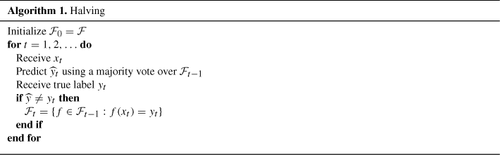
Theorem 25
The halving algorithm when run on a finite class![]() enjoys a mistake bound of
enjoys a mistake bound of ![]() .
.
In the non-realizable case, halving does not work directly but a suitable modification does. Since no function in the class can be guaranteed to be correct all the time, it does not make sense to eliminate functions that make mistakes. The crucial idea here is to keep weights for different functions in the class. Then, when a functions makes a mistake, it is not eliminated but its weight is multiplied by a factor of ![]() where
where ![]() is a parameter. The prediction are now taken using a weighted majority vote over all
is a parameter. The prediction are now taken using a weighted majority vote over all ![]() :
:
 (14.6)

Theorem 26
At any the end of any given round, let![]() be the number of mistakes made by a function
be the number of mistakes made by a function![]() so far. Then the number of mistakes M made by weighted majority so far is bounded as
so far. Then the number of mistakes M made by weighted majority so far is bounded as
![]()
In particular, using the uniform distribution![]() , we get
, we get
![]()
Proof
Fix a round index ![]() and let M and
and let M and ![]() be defined as the numbers of mistakes in the first T rounds. Let
be defined as the numbers of mistakes in the first T rounds. Let ![]() be the fraction of weights on the functions that made a mistake on round
be the fraction of weights on the functions that made a mistake on round ![]() . Since we make a mistake if and only if
. Since we make a mistake if and only if ![]() , we have
, we have
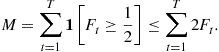 (14.7)
Define the total weight
![]()
At round t, the total weight changes as
![]()
Hence the final total weight is
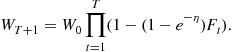
Note that ![]() . If the function f made
. If the function f made ![]() mistakes, its weight is
mistakes, its weight is
![]()
Since ![]() , we have
, we have
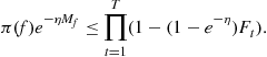
Taking negative logs of both sides reverses the inequality giving

Using the elementary but useful inequality ![]() gives
gives

Combining this with the bound (14.7) proves the theorem. ![]()
It turns out we can shave off a factor of 2 in the above mistake bound by using a randomized version of the weighted majority algorithm. Instead of taking the majority vote with the weights ![]() , we can consider a Gibbs classifier that chooses a function
, we can consider a Gibbs classifier that chooses a function ![]() randomly from
randomly from ![]() with probability proportional to
with probability proportional to ![]() and then outputs
and then outputs ![]() . This makes the number of mistakes a random variable but the bound (14.7) turns into an equality without the factor of 2. That is, for the randomized weighted majority algorithm
. This makes the number of mistakes a random variable but the bound (14.7) turns into an equality without the factor of 2. That is, for the randomized weighted majority algorithm

Thus we have the following result.
Theorem 27
Suppose that we change the weighted majority step(14.6)to the randomized weighted majority step
![]()
Then, this randomized version of weighted majority satisfies the expected mistake bound
![]()
1.14.6.5.2 Perceptron and winnow
We now consider two online algorithms that learn a linear threshold function. Perceptron is a classic algorithm that dates back to the 1960s. The Winnow algorithm was proposed by Littlestone [45] as a better alternative when there are many irrelevant features in the inputs.
Both algorithms follow the general schema given in Algorithm 3. Perceptron uses the additive update rule:
![]()
whereas Winnow uses a multiplicative update rule
![]()
where ![]() and
and ![]() denote entry wise multiplication and exponentiation respectively. The normalization constant
denote entry wise multiplication and exponentiation respectively. The normalization constant ![]() ensures that the weight vector remains a probability distribution. Also note that in Perceptron, we use the initialization
ensures that the weight vector remains a probability distribution. Also note that in Perceptron, we use the initialization ![]() whereas Winnow initializes
whereas Winnow initializes ![]() with the uniform distribution over the d features.
with the uniform distribution over the d features.
To give a mistake bound for Perceptron and Winnow, we will assume that we are in realizable case. That is, there is some weight vector ![]() that can perfectly classify all the examples that the learner sees. Moreover, we can assume that there is a margin available in the correct classifications. For a correct classification, it should simply be the case that
that can perfectly classify all the examples that the learner sees. Moreover, we can assume that there is a margin available in the correct classifications. For a correct classification, it should simply be the case that ![]() . The margin condition will ensure that there is a lower bound
. The margin condition will ensure that there is a lower bound ![]() such that
such that
![]() (14.8)
(14.8)
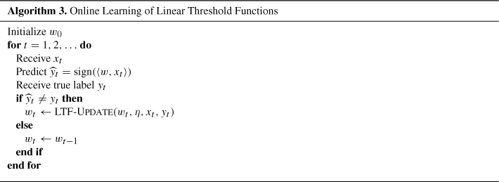
Theorem 28
Suppose there exists a![]() satisfying the margin condition(14.8). Then Perceptron with learning rate
satisfying the margin condition(14.8). Then Perceptron with learning rate![]() enjoys the mistake bound
enjoys the mistake bound
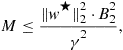
where![]() .
.
Proof
Let ![]() and note that the number
and note that the number ![]() of mistakes till time T is simply
of mistakes till time T is simply

where ![]() . Let us calculate how the inner product of
. Let us calculate how the inner product of ![]() with the vector
with the vector ![]() evolves. Note that we can write
evolves. Note that we can write
![]()
Thus, we have,

where the last step is due to the margin assumption (14.8). Summing the above inequality for ![]() yields
yields
![]()
Since ![]() and
and ![]() , we get
, we get
![]() (14.9)
(14.9)
Let us now try to upper bound ![]() . We have,
. We have,
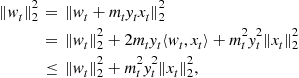
where the last line is true because ![]() when
when ![]() . Also note that
. Also note that ![]() , and
, and ![]() . Therefore,
. Therefore,
![]()
Summing this for ![]() gives
gives
![]()
Combining this with (14.9) gives
![]()
which gives us the final bound
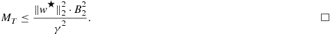
Theorem 29
Suppose there exists a![]() with positive entries that satisfies the margin condition(14.8). Let
with positive entries that satisfies the margin condition(14.8). Let![]() . Then Winnow enjoys the mistake bound
. Then Winnow enjoys the mistake bound
![]()
whenever

In particular, by setting![]() optimally, we get,
optimally, we get,
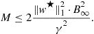
Proof
Let ![]() . Since
. Since ![]() (inequality is entrywise),
(inequality is entrywise), ![]() is a probability distribution. Moreover, Winnow maintains a probability distribution
is a probability distribution. Moreover, Winnow maintains a probability distribution ![]() at all times. We will track the progress of the algorithm using the relative entropy
at all times. We will track the progress of the algorithm using the relative entropy
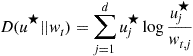
between ![]() and
and ![]() .
.
Suppose a mistake occurs at time t. Then we have,
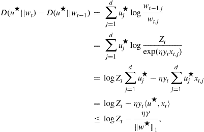 (14.10)
where the last step is due to the margin assumption (14.8). Note that ![]() .
. ![]()
For any ![]() and
and ![]() , we have the inequality
, we have the inequality
![]()
To see this consider a random variable Z that takes value ![]() with probability
with probability ![]() and takes value
and takes value ![]() with probability
with probability ![]() . Then the inequality above is claims that
. Then the inequality above is claims that ![]() which is indeed true by Jensen’s inequality. Using the inequality above, we have
which is indeed true by Jensen’s inequality. Using the inequality above, we have

where the last step is true because, in a mistake round, ![]() . Combining this bound on
. Combining this bound on ![]() with (14.10) gives us, on any mistake round,
with (14.10) gives us, on any mistake round,
![]()

Thus, for any round,
![]()
where ![]() . Summing this over
. Summing this over ![]() gives
gives
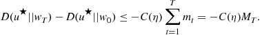
Since relative entropy is always non-negative ![]() . On the other hand,
. On the other hand,
Thus, we have
![]()
which gives, whenever ![]() ,
,
![]()
By choosing ![]() to maximize
to maximize ![]() , we get
, we get

which yields the bound

where
![]()
The second statement of the theorem now follows because ![]() for
for ![]() .
.
1.14.7 Beyond the basic probabilistic framework
Our overview of learning theory emphasized the classical setting in which a learning algorithm sees fully labeled data that is an iid draw from an unknown distribution. There are many extensions possible to this basic setting. We mention a few directions that are have been explored by researchers. Many of these continue to evolve actively as new results appear.
Richer Output Spaces: We mostly talked about classification and regression. One can certainly consider richer output spaces. The field of structured prediction[47] deals with exponentially large output spaces consisting of graphs, trees, or other combinatorials objects. Another output space that arises in ranking applications is the space of permutations of a finite set of objects. There has also been work on learning vector valued functions [48].
Learning with Dependent Data: The iid assumption has also been relaxed. Aldous and Vazirani [49], Gamarnik [50] consider Markov chains. Irle [51], Meir [52], Vidyasagar [17], Lozano et al. [53], Mohri and Rostamizadeh [54], Steinwart et al. [55] consider mixing processes. There is also a negative result [56] showing that there is no universally consistent learning algorithm for stationary ergodic processes.
Learning with Adversarially Generated Data: As in the mistake bound model, it is possible to develop a theory of learning from online adversarially generated data provided one defines learnability in terms of low regret

which compares the performance of the learner’s functions ![]() to the best function chosen in hindsight (note that the learner has to commit to
to the best function chosen in hindsight (note that the learner has to commit to ![]() seeing only examples till
seeing only examples till ![]() . Analogues of Rademacher complexity, covering numbers, and fat shattering dimension have been developed [57]. This topic has fascinating connections to information theory and game theory. See [21] for a comprehensive overview.
. Analogues of Rademacher complexity, covering numbers, and fat shattering dimension have been developed [57]. This topic has fascinating connections to information theory and game theory. See [21] for a comprehensive overview.
Active Learning: In active learning, we consider situations where the learner has some control over the data it uses to learn. This is in contrast to the basic iid model where the learner passively sees iid data drawn from a distribution. In particularly useful model of active learning, we assume that the learning has access to unlabeled points ![]() drawn iid from a distribution either all at one (a pool) or one at a time (a stream). The learner can only query for labels of examples in the pool or the stream. The label complexity of the learner is the number of label queries it needs to make in order to achieve a desired accuracy with a given level of confidence. In a lot of situations, unlabeled data is cheap and easy to get. So, it makes sense to charge the learner only for the number of labels it requires. The label complexity of different problems in an active learning has been studied (see, for example, [58] and references therein). Given the practical importance of reducing the number of labels required and the relatively unexplored nature of active learning, a lot remains to be done.
drawn iid from a distribution either all at one (a pool) or one at a time (a stream). The learner can only query for labels of examples in the pool or the stream. The label complexity of the learner is the number of label queries it needs to make in order to achieve a desired accuracy with a given level of confidence. In a lot of situations, unlabeled data is cheap and easy to get. So, it makes sense to charge the learner only for the number of labels it requires. The label complexity of different problems in an active learning has been studied (see, for example, [58] and references therein). Given the practical importance of reducing the number of labels required and the relatively unexplored nature of active learning, a lot remains to be done.
Semisupervised Learning: Semisupervised learning refers to learning with labeled data and large amounts of unlabeled data. A lot of work has been done in this area including methods that try to learn classifiers whose decision boundary passed through low density regions of the unlabeled data to graph based methods that use regularization to penalize functions that are nonsmooth along edges of a graph built from unlabeled data. For a good collection of articles on semisupervised learning, see the collection [59]. In the same collection, Balcan and Blum propose a PAC style framework for semisupervised learning.
Learning Multiple Tasks: In multitask learning, the learner is faced with learning multiple related tasks. Because of task relatedness, we expect the learner to require fewer samples when the tasks are learned together rather than separately. Many approaches try to encode task relatedness into a regularization function that couples all the tasks together. Some important advances in our theoretical understanding of multitask learning have been made ([60–63]) but a comprehensive theory, if one exists, remains to be found.
1.14.8 Conclusions and future trends
Understanding intelligence and constructing intelligent machines is a great scientific challenge. An understanding of learning is central to an understanding of intelligence. Whether we talk about learning on an evolutionary time scale or learning within the lifespan of an organism, learning plays a crucial role in the development of intelligent behavior. What learning theory has attempted to do so far is provide a solid mathematical framework within which to pose and solve questions regarding the process of learning. Admittedly, the most mature part of learning theory is the theory of supervised learning including classification and regression problems. But this is just a beginning rather than the end. We hope that future research will make learning theory much richer and applicable to a broader variety of problems in both natural and artificial systems.
Learning theory is an interdisciplinary field. It draws ideas and inspiration from a variety of disciplines including biology, computer science, economics, philosophy, psychology, statistical physics, and statistics. It attempts to achieve clarity and rigor by using the language of mathematics to precisely state assumptions and prove results. We expect that interdisciplinary cross-fertilization of ideas will continue to enrich and give new directions to learning theory. For example, learning theory has much to contribute to problems arising in diverse areas such as control [17] and dynamical systems [64], learning in games [65], privacy [66], evolution [67], and mechanism design [68].
Glossary
AdaBoost Acronym for Adaptive Boosting, a popular boosting algorithm
Bayes classifier In classification problems with 0–1 loss, a classifier with the least risk
Boosting The process of converting a weak learning algorithm (that is, one that outputs classifiers whose performance is just a little bit better than random guessing) into a strong one
Concentration inequality A probabilistic inequality stating that some random variable will not deviate too far from its mean or median
Excess risk The difference between the risk of a given function and the minimum possible risk over a function class
Empirical risk Same as risk except that the expectation under the unknown data distribution is replaced with an empirical average over the samples observed
Empirical risk minimization A learning rule that minimizes the empirical risk to choose a prediction function
ERM Empirical Risk Minimization
Fat shattering dimension A scale sensitive generalization of the VC dimension.
Generalization error bound An upper bound stating that the risk of a learning rule is not going to differ too much from its empirical risk
Kernel A symmetric positive semidefinite function
Littlestone dimension A combinatorial quantity associated with a class of binary valued functions. Plays a fundamental role in determining worst case bounds in the online mistake bound model
Loss function A function used to measure the quality of a prediction given the true label.
Mistake bound model A model of learning that, unlike the PAC model, does not assume anything about the way data is generated
Model selection The task of selecting an appropriate statistical model from a family based on available data
PAC model A computational model for analyzing the resources (time, memory, samples) required for performing learning tasks. Originally defined for the task of binary classification using the 0–1 loss. The acronym PAC stands for “Probably Approximately Correct”
Rademacher complexity A quantity associated with a function class that measures its capacity to overfit by measuring how well the function class can fit randomly generated ![]() signs
signs
Regression function In regression problems with the squares loss, the prediction function with the least risk
Reproducing kernel Hilbert space A Hilbert space of functions for which there exists a kernel with the reproducing property: point evaluations of functions can be written as linear functionals
Risk The expected loss of a prediction function under the underlying unknown distribution generating input, output pair
Sample complexity The number of samples requires to achieve a given level of accuracy (usually with high probability)
Sample compression An approach to obtaining generalization error bounds for algorithms whose output can be reconstructed from a small number of examples belonging to the original sample
Stability The property of a learning algorithm that ensures that its output does not change much if the training data set is changed slightly
Supervised learning The task of learning a functional dependence between an input space and an output or label space using given examples of input, output pairs
Universal consistency The property of a learning rule to converge to the minimum possible risk as the number of samples grows to infinity
Vapnik-Chervonenkis dimension A combinatorial quantity associated with a binary valued function class that serves as a measure of the capacity of the function class to overfit the data
VC dimension Vapnik-Chervonenkis dimension
Relevant Theory: Machine Learning
See this Volume, Chapter 14 Learning Theory
See this Volume, Chapter 15 Neural Networks
See this Volume, Chapter 16 Kernel Methods and SVMs
See this Volume, Chapter 17 Online Learning in Reproducing Kernel Hilbert Spaces
See this Volume, Chapter 18 Introduction to Probabilistic Graphical Models
See this Volume, Chapter 20 Clustering
See this Volume, Chapter 22 Semi-supervised Learning
See this Volume, Chapter 23 Sparsity-Aware Learning and Compressed Sensing: An Overview
See this Volume, Chapter 25 A Tutorial on Model Selection
Relevant websites
• Scholarpedia has a section devoted to machine learning containing links to articles written by leading researchers.
http://www.scholarpedia.org/article/Category:Machine_learning/
• The Encyclopedia of Machine Learning is a valuable online resource available through subscription.
http://www.springerlink.com/content/978-0-387-30768-8/
• The Journal of Machine Learning Research a leading open access journal publishing high quality articles in machine learning and related topics.
http://jmlr.csail.mit.edu/
• Another high quality journal publishing articles on machine learning and related topics is Machine Learning.
www.springer.com/computer/ai/journal/10994
• There is a Google group for postings of possible interest to learning theory researchers.
http://groups.google.com/group/learning-theory/
• The website of the International Machine Learning Society. The society organizes the annual International Conference on Machine Learning (ICML).
http://www.machinelearning.org/
• The website of the Association for Computational Learning. The association organizes the annual Conference on Learning Theory (COLT).
http://seed.ucsd.edu/joomla/
• The website of the Neural Information Processing Systems (NIPS) Foundation. The foundation organizes the annual NIPS conference.
http://nips.cc/
• The arXiv is good way to find recent preprints in machine learning and learning theory.
http://arxiv.org/list/cs.LG/recent/
References
1. Turing AM. Computing machinery and intelligence. Mind. 1950;59:433–460.
2. McCulloch WS, Pitts W. A logical calculus of the ideas immanent in neural nets. Bulletin of Mathematical Biophysics. 1943;5:115–137.
3. Samuels AL. Some studies in machine learning using the game of checkers. IBM J Res Develop. 1959;3(3):210–233.
4. Rosenblatt F. Two theorems of statistical separability in the perceptron. In: Proceedings of a Symposium on the Mechanization of Thought Processes. London: Her Majesty’s Stationary Office; 1959;421–456.
5. Novikoff ABJ. On convergence proofs for perceptrons. In: Proceedings of the Symposium on the Mathematical Theory of Automata (New York, 1962). 1963;615–622.
6. Vapnik V. Statistics for engineering and information science The Nature of Statistical Learning Theory second ed. Springer 2000.
7. Rumelhart DE, Hinton G, Williams RJ. Learning representations by back-propagating errors. Nature. 1986;323:533–536.
8. Valiant LG. A theory of the learnable. J ACM. 1984;27(11):1134–1142.
9. Cortes C, Vapnik VN. Support-vector networks. Mach Learn. 1995;20(3):273–295.
10. Freund Y, Schapire RE. A decision-theoretic generalization of online-learning and an application to boosting. In: Proceedings of the Second European Conference on Computational Learning Theory. 1995;23–37.
11. Stone CJ. Consistent nonparametric regression. Ann Stat. 1977;5(4):595–620.
12. Anthony M, Biggs N. Computational Learning Theory: An Introduction, Number 30 in Cambridge Tracts in Computer Science. Cambridge University Press 1997.
13. Anthony M, Bartlett PL. Neural Network Learning: Theoretical Foundations. Cambridge University Press 1999.
14. Devroye L, Györfi L, Lugosi G. In: A Probabilistic Theory of Pattern Recognition. Springer 1996; Stochastic Modelling and Applied Probability vol. 31.
15. Vapnik V. Estimation of Dependences Based on Empirical Data; Empirical Inference Science: Afterword of 2006. second ed. Springer 2006; Reprint of 1982 edition with afterword of 2006.
16. Vapnik V. Adaptive and learning systems for signal processing, communications, and control Statistical Learning Theory Wiley 1998.
17. Vidyasagar M. Learning and Generalization: With Application to Neural Networks, Communications and control engineering. second ed. Springer 2003.
18. Natarajan BK. Machine Learning: A Theoretical Approach. Morgan Kauffmann 1991.
19. Cucker F, Zhou D-X. Learning Theory: An Approximation Theory Viewpoint Cambridge Monographs on Applied and Computational Mathematics Cambridge University Press 2007.
20. Kearns MJ, Vazirani UV. An Introduction to Computational Learning Theory. MIT Press 1994.
21. Cesa-Bianchi N, Lugosi G. Prediction, Learning, and Games. Cambridge University Press 2006.
22. Györfi L, Kohler M, Krzyjak A, Walk H. A Distribution Free Theory of Nonparametric Regression Springer Series in Statistics Springer 2002.
23. Hastie T, Tibshirani R, Friedman J. The Elements of Statistical Learning Springer Series in Statistics second ed. Springer 2009.
24. Massart P. Concentration inequalities and model selection. In: Springer 2007; Lecture Notes in Mathematics. vol. 1896.
25. Bartlett PL, Mendelson S. Rademacher and gaussian complexities: Risk bounds and structural results. J Mach Learn Res. 2002;3:463–482.
26. Ambroladze A, Parrado-Hernández E, Shawe-Taylor J. Complexity of pattern classes and the lipschitz property. Theor Comp Sci. 2007;382(3):232–246.
27. Dudley RM. The sizes of compact subsets of Hilbert space and continuity of Gaussian processes. J Funct Anal. 1967;1(3):290–330.
28. Vapnik VN, Ya A, Chervonenkis AYa. On the uniform convergence of relative frequencies of event to their probabilities. Soviet Mathematics Doklady. 1968;9:915–918.
29. Sauer N. On the density of families of sets. J Comb Theory A. 1972;13:145–147.
30. Shelah Saharon. A combinatorial problem; stability and order for models and theories in infinitary languages. Pac J Math. 1972;41:247–261.
31. Haussler D. Sphere packing numbers for subsets of the boolean n-cube with bounded vapnik-chervonenkis dimension. J Comb Theory A. 1995;69(2):217–232.
32. Alon N, Ben-David S, Cesa-Bianchi N, Haussler D. Scale-sensitive dimensions, uniform convergence, and learnability. J ACM. 1997;44(4):615–631.
33. Warmuth MK. Sample compression, learnability, and the vapnik-chervonenkis dimension. In: Proceedings of the Third European Conference on Computational Learning Theory. 1997;1–2.
34. Bousquet O, Elisseeff A. Stability and generalization. J Mach Learn Res. 2002;2:499–526.
35. Kutin S, Niyogi P. Almost-everywhere algorithmic stability and generalization error. In: Proceedings of the 18th Conference on Uncertainty in, Artificial Intelligence. 2002;275–282.
36. Mukherjee S, Niyogi P, Poggio T, Rifkin RM. Learning theory: stability is sufficient for generalization and necessary and sufficient for consistency of empirical risk minimization. Adv Comput Math. 2006;25(1–3):161–193.
37. Shalev-Shwartz S, Shamir O, Srebro N, Sridharan K. Learnability, stability and uniform convergence. J Mach Learn Res. 2010;11:2635–2670.
38. McAllester David A. PAC-Bayesian stochastic model selection. Mach Learn. 2003;51(1):5–21.
39. Schapire Robert E. The strength of weak learnability. Mach Learn. 1990;5:197–227.
40. Freund Y. Boosting a weak learning algorithm by majority. Info Comput. 1995;121(2):256–285.
41. Freund Y, Schapire RE. Game theory, on-line prediction and boosting. In: Proceedings of the Ninth Annual Conference on Computational Learning Theory. 1996;325–332.
42. Angluin D, Laird PD. Learning from noisy examples. Mach Learn. 1987;2(4):343–370.
43. Kearns M. Efficient noise-tolerant learning from statistical queries. J ACM. 1998;45(6):983–1006.
44. Feldman V, Gopalan P, Khot S, Ponnuswami AK. On agnostic learning of parities, monomials, and halfspaces. SIAM J Comput. 2009;39(2):606–645.
45. Littlestone N. Learning quickly when irrelevant attributes abound: a new linear-threshold algorithm. Mach Learn. 1987;2(4):285–318.
46. Ben-David S, Pál D, Shalev-Shwartz S. Agnostic online learning. In: Proceedings of the 22nd Annual Conference on Learning Theory. 2009.
47. Bakir GH, Hofmann T, Schölkopf B, Smola AJ, Taskar Ben, Vishwanathan SVN. Predicting Structured Data. MIT Press 2007.
48. Micchelli CA, Pontil M. On learning vector-valued functions. Neural Comput. 2005;17(1):177–204.
49. Aldous D, Vazirani V. A Markovian extension of Valiant’s learning model. In: 1990;392–396. Proceedings of the 31st Annual Symposium on Foundations of Computer Science. vol. 1.
50. Gamarnik D. Extension of the PAC framework to finite and countable Markov chains. In: Proceedings of the twelfth annual conference on Computational learning theory. 1999;308–317.
51. Irle A. On the consistency in nonparametric estimation under mixing assumptions. J Multivar Anal. 1997;60:123–147.
52. Meir R. Nonparametric time series prediction through adaptive model selection. Mach Learn. 2000;39(1):5–34.
53. Lozano A, Kulkarni S, Schapire R. Convergence and consistency of regularized boosting algorithms with stationary ![]() -mixing observations. Adv Neural Inform Process Syst. 2006;18:819–826.
-mixing observations. Adv Neural Inform Process Syst. 2006;18:819–826.
54. Mohri M, Rostamizadeh A. Rademacher complexity bounds for non-i.i.d processes. Advances in Neural Information Processing. 2009;21:1097–1104.
55. Steinwart I, Hush D, Scovel C. Learning from dependent observations. J Multivar Anal. 2009;100(1):175–194.
56. Nobel A. Limits to classification and regression estimation from ergodic processes. Ann Stat. 1999;27(1):262–273.
57. Rakhlin A, Sridharan K, Tewari A. Online learning: Random averages, combinatorial parameters, and learnability. Adv Neural Inform Process Syst. 2010;23:1984–1992.
58. Hanneke S. Rates of convergence in active learning. Ann Stat. 2011;39(1):333–361.
59. Chapelle O, Schölkopf B, Zien A, eds. Semi-Supervised Learning. Cambridge, MA: MIT Press; 2006.
60. Baxter J. A model of inductive bias learning. J Artif Intell Res. 2000;12:149–198.
61. Caruana R. Multitask learning. Mach Learn. 1997;28(1):41–75.
62. Evgeniou T, Micchelli CA, Pontil M. Learning multiple tasks with kernel methods. J Mach Learn Res. 2005;6:615–637.
63. Maurer A. Bounds for linear multi-task learning. J Mach Learn Res. 2006;7:117–139.
64. Campi M, Kumar PR. Learning dynamical systems in a stationary environment. Syst Control Lett. 1998;34(3):125–132.
65. Peyton Young H. Strategic Learning and Its Limits. Oxford University Press 2004.
66. Balcan M-F, Blum A, Fine S, Mansour Y. Distributed learning, communication complexity and privacy. In: 2012;26.1–26.22. Proceedings of the 25th Annual Conference on Learning Theory, JMLR Workshop and Conference Proceedings. vol. 23.
67. Valiant LG. Evolvability. J ACM. 2009;56.
68. Balcan M-F, Blum A, Hartline JD, Mansour Y. Reducing mechanism design to algorithm design via machine learning. J Comp Syst Sci. 2008;74(8):1245–1270.