
Unsupervised Learning Algorithms and Latent Variable Models: PCA/SVD, CCA/PLS, ICA, NMF, etc.
Andrzej Cichocki, Laboratory for Advanced Brain Signal Processing, RIKEN, Brain Science Institute, Wako-shi, Saitama 3510198, Japan, [email protected]
Abstract
Constrained matrix and tensor factorizations, also called penalized matrix/tensor decompositions play a key role in Latent Variable Models (LVM), Multilinear Blind Source Separation (MBSS), and (multiway) Generalized Component Analysis (GCA) and they are important unifying topics in signal processing and linear and multilinear algebra. This chapter introduces basic linear and multilinear models for matrix and tensor factorizations and decompositions. The “workhorse” of this chapter consists of constrained matrix decompositions and their extensions, including multilinear models which perform multiway matrix or tensor factorizations, with various constraints such as orthogonality, statistical independence, nonnegativity and/or sparsity. The constrained matrix and tensor decompositions are very attractive because they take into account spatial, temporal and/or spectral information and provide links among the various extracted factors or latent variables while providing often physical or physiological meanings and interpretations. In fact matrix/tensor decompositions are important techniques for blind source separation, dimensionality reduction, pattern recognition, object detection, classification, multiway clustering, sparse representation and coding and data fusion.
Keywords
Unsupervised learning; Multiway generalized component analysis (GCA); Multilinear blind source separation (MBSS); Multilinear independent component analysis (MICA); Constrained matrix and tensor decompositions; CP/PARAFAC and Tucker models; Nonnegative matrix and tensor factorizations (NMF/NTF); Multi-block data analysis; Linked multiway component analysis
1.21.1 Introduction and of problems statement
Matrix factorizations and their extensions to tensor (multiway arrays) factorizations and decompositions have become prominent techniques for Latent Variable Models (LVM), linear and Multiway or Multilinear Blind Source Separation (MBSS), and (multiway) Generalized Component Analysis (GCA) (especially, multilinear Independent Component Analysis (ICA), Nonnegative Matrix and Tensor Factorizations (NMF/NTF), Smooth Component Analysis (SmoCA), and Sparse Component Analysis (SCA). Moreover, matrix and tensor decompositions have many other applications beyond blind source separation, especially for feature extraction, classification, dimensionality reduction and multiway clustering. The recent trends in MBSS and GCA are to consider problems in the framework of matrix and tensor factorizations or more general multi-dimensional data for signal decomposition within probabilistic generative models and exploit a priori knowledge about the true nature, diversities, morphology or structure of latent (hidden) variables or sources such as spatio-temporal-spectral decorrelation, statistical independence, nonnegativity, sparseness, smoothness or lowest possible complexity. The goal of MBSS can be considered as estimation of true physical sources and parameters of a mixing system, while the objective of GCA is to find a reduced (or hierarchical and structured) component representation for the observed (sensor) multi-dimensional data, that can be interpreted as physically or physiologically meaningful coding or blind signal decomposition. The key issue is to find such a transformation (or coding) which has true physical meaning and interpretation. In this chapter we briefly review some efficient unsupervised learning algorithms for linear and multilinear blind source separation, blind source extraction and blind signals decomposition, using various criteria, constraints and assumptions. Moreover, we briefly overview emerging models and approaches for constrained matrix/tensor decompositions with applications to group and linked multilinear BSS/ICA, feature extraction, multiway Canonical Correlation Analysis (CCA), and Partial Least Squares (PLS) regression problems.
Although the basic models for matrix and tensor (i.e., multiway array) decompositions and factorizations, such as Tucker and Canonical Polyadic (CP) decomposition models, were proposed long a time ago [1–7], they have recently emerged as promising tools for the exploratory analysis of large-scale and multi-dimensional data in diverse applications, especially, for dimensionality reduction, multilinear independent component analysis, feature extraction, classification, prediction, and multiway clustering [5,8–12]. By virtue of their multiway nature, tensors constitute powerful tools for the analysis and fusion of large-scale, multi-modal massive data, together with a mathematical backbone for the discovery of underlying hidden complex data structures [8,13].
The problem of separating or extracting source signals from a sensor array, without knowing the transmission channel characteristics and the sources, is addressed by a number of related BSS or GCA methods such as ICA and its extensions: Topographic ICA, Multilinear ICA, Kernel ICA, Tree-dependent Component Analysis, Multi-resolution Subband Decomposition ICA [13–18], Non-negative Matrix Factorization (NMF) [19,20], Sparse Component Analysis (SCA) [21–25], and Multi-channel Morphological Component Analysis (MCA) [26,27].
The mixing and filtering processes of the unknown input sources ![]() may correspond to different mathematical or physical models, depending on the specific applications [17,28]. Most linear BSS models can be expressed algebraically in their simplest forms as some specific form of a constrained matrix factorization: Given observation (often called sensor or input) data matrix
may correspond to different mathematical or physical models, depending on the specific applications [17,28]. Most linear BSS models can be expressed algebraically in their simplest forms as some specific form of a constrained matrix factorization: Given observation (often called sensor or input) data matrix ![]() , we perform the matrix factorization (see Figure 21.1a):
, we perform the matrix factorization (see Figure 21.1a):
![]() (21.1)
(21.1)
where ![]() represents the unknown mixing matrix,
represents the unknown mixing matrix, ![]() is an unknown matrix representing errors or noises,
is an unknown matrix representing errors or noises, ![]() contains the corresponding latent (hidden) components that give the contribution of each basis vector, T is the number of available samples, I is the number of observations and J is the number of sources or components.
contains the corresponding latent (hidden) components that give the contribution of each basis vector, T is the number of available samples, I is the number of observations and J is the number of sources or components.
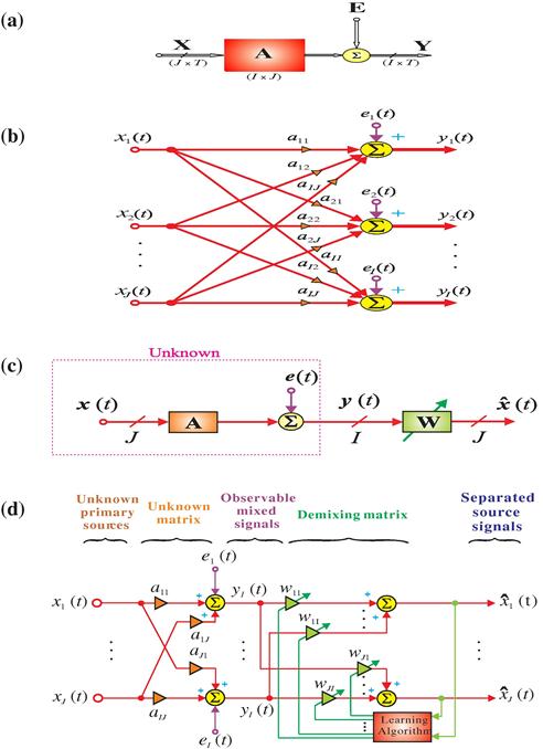
Figure 21.1 Basic linear (instantaneous) BSS model: (a) Block diagram expressed as a matrix factorization: ![]() , (b) its detailed model, (c) BSS via separating (demixing) matrix
, (b) its detailed model, (c) BSS via separating (demixing) matrix ![]() , and (d) its detailed model.
, and (d) its detailed model.
In general the number of source signals J is unknown, and it can be larger, equal or smaller than the number of observations. The above model can be written in an equivalent scalar (element-wise) form (see Figure 21.1b):
 (21.2)
Usually, the latent components represent unknown source signals with specific statistical properties or temporal structures and matrices have clear statistical properties and meanings. For example, the rows of the matrix ![]() that represent unknown sources or components should be statistically independent for ICA, sparse for SCA [21–24,29], nonnegative for NMF [8], or have other specific and additional morphological properties such as smoothness, continuity, or orthogonality [14,16,27].
that represent unknown sources or components should be statistically independent for ICA, sparse for SCA [21–24,29], nonnegative for NMF [8], or have other specific and additional morphological properties such as smoothness, continuity, or orthogonality [14,16,27].
In many signal processing applications the data matrix ![]() is represented by vectors
is represented by vectors ![]() of multiple measurements or recordings for a set of discrete time points t. As mentioned above, the compact aggregated matrix Eq. (21.1) can be written in a vector form as a system of linear equations (see Figure 21.1c), that is,
of multiple measurements or recordings for a set of discrete time points t. As mentioned above, the compact aggregated matrix Eq. (21.1) can be written in a vector form as a system of linear equations (see Figure 21.1c), that is,
![]() (21.3)
(21.3)
where ![]() is a vector of the observed signals at the discrete time point t whereas
is a vector of the observed signals at the discrete time point t whereas ![]() is a vector of unknown sources at the same time point.
is a vector of unknown sources at the same time point.
In order to estimate sources, sometimes we try first to identify the mixing matrix ![]() or its (pseudo)-inverse (unmixing) matrix
or its (pseudo)-inverse (unmixing) matrix ![]() and then estimate the sources. Usually, the inverse (unmixing) system should be adaptive in such a way that it has some tracking capability in a nonstationary environment (see Figure 21.1d). We assume here that only the sensor vectors
and then estimate the sources. Usually, the inverse (unmixing) system should be adaptive in such a way that it has some tracking capability in a nonstationary environment (see Figure 21.1d). We assume here that only the sensor vectors ![]() are available and we need to estimate the parameters of the unmixing system online. This enables us to perform indirect identification of the mixing matrix
are available and we need to estimate the parameters of the unmixing system online. This enables us to perform indirect identification of the mixing matrix ![]() (for
(for ![]() ) by estimating the separating matrix
) by estimating the separating matrix ![]() , where the symbol
, where the symbol ![]() denotes the Moore–Penrose pseudo-inverse, and simultaneously estimate the sources. In other words, for
denotes the Moore–Penrose pseudo-inverse, and simultaneously estimate the sources. In other words, for ![]() the original sources can be estimated by the linear transformation
the original sources can be estimated by the linear transformation
![]() (21.4)
(21.4)
However, instead of estimating the source signals by projecting the observed signals by using the demixing matrix ![]() , it is often more convenient to identify an unknown mixing matrix A (e.g., when the demixing system does not exist, especially when the system is underdetermined, i.e., the number of observations is lower than the number of source signals:
, it is often more convenient to identify an unknown mixing matrix A (e.g., when the demixing system does not exist, especially when the system is underdetermined, i.e., the number of observations is lower than the number of source signals: ![]() ) and then estimate the source signals by exploiting some a priori information about the source signals by applying a suitable optimization procedure.
) and then estimate the source signals by exploiting some a priori information about the source signals by applying a suitable optimization procedure.
There appears to be something magical about the BSS since we are estimating the original source signals without knowing the parameters of the mixing and/or filtering processes. It is difficult to imagine that one can estimate this at all. In fact, without some a priori knowledge it is not possible to uniquely estimate the original source signals. However, one can usually estimate them up to certain indeterminacies. In mathematical terms these indeterminacies and ambiguities can be expressed as arbitrary scaling and permutations of the estimated source signals. Let ![]() denote a specific BSS algorithm, then it holds that
denote a specific BSS algorithm, then it holds that
![]() (21.5)
(21.5)
where ![]() and
and ![]() are the permutation matrix and a diagonal scaling matrix (with nonzero entries), respectively. As a result, the original source signals represented by the rows of
are the permutation matrix and a diagonal scaling matrix (with nonzero entries), respectively. As a result, the original source signals represented by the rows of ![]() are recovered as
are recovered as ![]() with the unavoidable ambiguities of scaling and permutations. If the BSS via constrained matrix factorization leads to the estimation of true components (sources) with arbitrary scaling and permutations, we call such factorization essentially unique. These indeterminacies preserve, however, the waveforms of the original sources. Although these indeterminacies seem to be rather severe limitations, in a great number of applications these limitations are not crucial, since the most relevant information about the source signals is contained in the temporal waveforms or time–frequency patterns of the source signals and usually not in their amplitudes or the order in which they are arranged in the system output. For some models, however, there is no guarantee that the estimated or extracted signals will have exactly the same waveforms as the source signals, and then the requirements must be sometimes further relaxed to the extent that the extracted waveforms are distorted (i.e., time delayed, filtered, or convolved) versions of the primary source signals.
with the unavoidable ambiguities of scaling and permutations. If the BSS via constrained matrix factorization leads to the estimation of true components (sources) with arbitrary scaling and permutations, we call such factorization essentially unique. These indeterminacies preserve, however, the waveforms of the original sources. Although these indeterminacies seem to be rather severe limitations, in a great number of applications these limitations are not crucial, since the most relevant information about the source signals is contained in the temporal waveforms or time–frequency patterns of the source signals and usually not in their amplitudes or the order in which they are arranged in the system output. For some models, however, there is no guarantee that the estimated or extracted signals will have exactly the same waveforms as the source signals, and then the requirements must be sometimes further relaxed to the extent that the extracted waveforms are distorted (i.e., time delayed, filtered, or convolved) versions of the primary source signals.
In some applications the mixing matrix ![]() is ill-conditioned. In such cases some special models and algorithms should be applied. Although some decompositions or matrix factorizations provide an exact reconstruction of the data (i.e.,
is ill-conditioned. In such cases some special models and algorithms should be applied. Although some decompositions or matrix factorizations provide an exact reconstruction of the data (i.e., ![]() ), we will consider here constrained factorizations which are approximative in nature. In fact, many problems in signal and image processing can be solved in terms of matrix factorizations. However, different cost functions and imposed constraints may lead to different types of matrix factorizations.
), we will consider here constrained factorizations which are approximative in nature. In fact, many problems in signal and image processing can be solved in terms of matrix factorizations. However, different cost functions and imposed constraints may lead to different types of matrix factorizations.
The BSS problems are closely related to the concept of linear inverse problems or more generally, to solving a large ill-conditioned system of linear equations (overdetermined or underdetermined), where it is required to estimate the vectors ![]() (also in some cases to identify the matrix
(also in some cases to identify the matrix ![]() ) from noisy data [14,30,31]. Physical systems are often contaminated by noise, thus, our task is generally to find an optimal and robust solution in a noisy environment. Wide classes of extrapolation, reconstruction, estimation, approximation, interpolation, and inverse problems can be converted into minimum norm problems of solving underdetermined systems of linear Eqs. (21.1) for
) from noisy data [14,30,31]. Physical systems are often contaminated by noise, thus, our task is generally to find an optimal and robust solution in a noisy environment. Wide classes of extrapolation, reconstruction, estimation, approximation, interpolation, and inverse problems can be converted into minimum norm problems of solving underdetermined systems of linear Eqs. (21.1) for ![]() [14,31]. Generally speaking, in signal processing applications, an overdetermined (
[14,31]. Generally speaking, in signal processing applications, an overdetermined (![]() ) system of linear Eqs. (21.1) describes filtering, enhancement, deconvolution and identification problems, while the underdetermined case describes inverse and extrapolation problems [14,30]. Although many different BSS criteria and algorithms are available, most of them exploit various diversities or constraints imposed for estimated components and/or factor matrices such as orthogonality, mutual independence, nonnegativity, sparsity, smoothness, predictability or lowest complexity. By diversities we usually mean different morphological characteristics or features of the signals.
) system of linear Eqs. (21.1) describes filtering, enhancement, deconvolution and identification problems, while the underdetermined case describes inverse and extrapolation problems [14,30]. Although many different BSS criteria and algorithms are available, most of them exploit various diversities or constraints imposed for estimated components and/or factor matrices such as orthogonality, mutual independence, nonnegativity, sparsity, smoothness, predictability or lowest complexity. By diversities we usually mean different morphological characteristics or features of the signals.
More sophisticated or advanced approaches for GCA use combinations or the integration of various diversities, in order to separate or extract sources with various constraints, morphology, structures, or statistical properties, and to reduce the influence of noise and undesirable interferences [14,32].
All the above-mentioned BSS models are usually based on a wide class of unsupervised or semi-supervised learning algorithms. Unsupervised learning algorithms try to discover a structure underlying a data set, extract the meaningful features, and find useful representations of the given data. Since data can always be interpreted in many different ways, some knowledge is needed to determine which features or properties best represent true latent (hidden) components. For example, PCA finds a low-dimensional representation of the data that captures most of its variance. On the other hand, SCA tries to explain the data as a mixture of sparse components (usually, in the time–frequency domain), and NMF seeks to explain the data by parts-based localized additive representations (with nonnegativity constraints).
Most linear BSS or GCA models can be represented as constrained bilinear matrix factorization problems, with suitable constraints imposed on the component matrix:
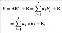 (21.6)
where ![]() is a known data matrix (representing observations or measurements),
is a known data matrix (representing observations or measurements), ![]() represents errors or noise,
represents errors or noise, ![]() is the unknown full column rank mixing (basis) matrix with J basis vectors
is the unknown full column rank mixing (basis) matrix with J basis vectors ![]() , and
, and ![]() represent the unknown components, latent variables or sources
represent the unknown components, latent variables or sources ![]() (see Figure 21.2).
(see Figure 21.2).

Figure 21.2 Bilinear BSS model. The data matrix ![]() is approximately represented by a sum or linear combination of rank-1 matrices
is approximately represented by a sum or linear combination of rank-1 matrices ![]() . The objective is to estimate all vectors
. The objective is to estimate all vectors ![]() and
and ![]() and the optimal index (rank) J. In general such decomposition is not unique, and we need to impose various constraints (e.g., nonnegativity, orthogonality, independence, or sparseness) to extract unique components with desired diversities or properties.
and the optimal index (rank) J. In general such decomposition is not unique, and we need to impose various constraints (e.g., nonnegativity, orthogonality, independence, or sparseness) to extract unique components with desired diversities or properties.
Note that we have symmetry of the factorization: For Eq. (21.6) we could write ![]() , so the meaning of “sources” and “mixture” are often somewhat arbitrary.
, so the meaning of “sources” and “mixture” are often somewhat arbitrary.
The unknown components usually have clear statistical properties and meaning. For example, the columns of the matrix ![]() should be as statistically mutually independent as possible, or sparse, piecewise smooth, and/or nonnegative, etc., according to the physical meaning of the components, and to research the field from which the data are collected. The BSS methods estimate these components maximizing the a priori information by imposing proper constraints on the components, then leading to various categories of BSS, such as ICA, SCA, SmoCA, NMF, etc. [8,14,33,34].
should be as statistically mutually independent as possible, or sparse, piecewise smooth, and/or nonnegative, etc., according to the physical meaning of the components, and to research the field from which the data are collected. The BSS methods estimate these components maximizing the a priori information by imposing proper constraints on the components, then leading to various categories of BSS, such as ICA, SCA, SmoCA, NMF, etc. [8,14,33,34].
Very often multiple subject, multiple task data sets can be represented by a set of data matrices ![]() . It is therefore necessary to perform simultaneous constrained matrix factorizations:
. It is therefore necessary to perform simultaneous constrained matrix factorizations:
![]() (21.7)
(21.7)
subject to various additional constraints (e.g., ![]() for all n, and their columns are mutually independent and/or sparse). This problem is related to various models of group ICA, with suitable pre-processing, dimensionality reduction and post-processing procedures [35–37]. This form of factorization is typical for EEG/MEG related data for multi-subjects, multi-tasks, while the factorization for the transposed of
for all n, and their columns are mutually independent and/or sparse). This problem is related to various models of group ICA, with suitable pre-processing, dimensionality reduction and post-processing procedures [35–37]. This form of factorization is typical for EEG/MEG related data for multi-subjects, multi-tasks, while the factorization for the transposed of ![]() is typical for fMRI data [35–38].
is typical for fMRI data [35–38].
The multilinear BSS concept introduced in Section 1.21.5.4 is more general and flexible than the group ICA, since various constraints can be imposed on the component matrices for different modes (i.e., not only mutual independence but also nonnegativity, sparseness, smoothness or orthogonality). There are neither theoretical nor experimental reasons why statistical independence (used by ICA) should be the only one right concept to be used to extract latent components [33]. In real world scenarios, latent (hidden) components have various complex properties and features. In other words, true unknown components are seldom all statistically independent. Therefore, if we apply only one criterion like ICA, we may fail to extract all desired components with correct interpretations. Rather we need to apply the fusion of several strategies by employing several suitably chosen criteria and their associated learning algorithms to extract all desired components for specific modes [8,33]. For these reasons we often consider the multilinear BSS methods, which exploit multiple criteria or diversities for the component matrices for various modes, rather than only statistical independence (see Section 1.21.5).
1.21.2 PCA/SVD and related problems
Principal Component Analysis (PCA) and Singular Value Decomposition (SVD) are well established tools with applications virtually in all areas of science, machine learning, signal processing, engineering, genetics and neural computation, to name just a few, where large data sets are encountered [39,40]. The basic aim of PCA is to find a few linear combinations of variables, called principal components, which point in orthogonal directions while explaining as much of the variance of the data as possible.
PCA is perhaps one of the oldest and best-known technique form multivariate analysis and data mining. It was introduced by Pearson, who used it in a biological context and further developed by Hotelling in research work related psychometry. PCA was also developed independently by Karhunen in the context of probability theory and was subsequently generalized by Loève (see [14,39,41] and references therein). The purpose of PCA is to derive a relatively small number of uncorrelated linear combinations (principal components) of a set of random zero-mean variables ![]() , while retaining as much of the information from the original variables as possible.
, while retaining as much of the information from the original variables as possible.
Following are several of the objectives of PCA/SVD:
2. determination of linear combinations of variables;
3. feature selection: the choice of the most useful variables;
4. visualization of multi-dimensional data;
Often the principal components (PCs) (i.e., directions on which the input data has the largest variance) are usually regarded as important or significant, while those components with the smallest variance called minor components (MCs) are usually regarded as unimportant or associated with noise. However, in some applications, the MCs are of the same importance as the PCs, for example, in the context of curve or surface fitting or total least squares (TLS) problems.
Generally speaking, PCA is often related and motivated by the following two problems:
1. Given random vectors ![]() , with finite second order moments and zero mean, find the reduced J-dimensional (
, with finite second order moments and zero mean, find the reduced J-dimensional (![]() ) linear subspace that minimizes the expected distance of
) linear subspace that minimizes the expected distance of ![]() from the subspace. This problem arises in the area of data compression, where the task is to represent all the data with a reduced number of parameters while assuring minimum distortion due to the projection.
from the subspace. This problem arises in the area of data compression, where the task is to represent all the data with a reduced number of parameters while assuring minimum distortion due to the projection.
2. Given random vectors ![]() , find the J-dimensional linear subspace that captures most of the variance of the data. This problem is related to feature extraction, where the objective is to reduce the dimension of the data while retaining most of its information content.
, find the J-dimensional linear subspace that captures most of the variance of the data. This problem is related to feature extraction, where the objective is to reduce the dimension of the data while retaining most of its information content.
It turns out that both problems have the same optimal solution (in the sense of least-squares error), which is based on the second order statistics (SOS), in particular, on the eigen structure of the data covariance matrix.
PCA is designed for a general random variable regardless whether it is of zero mean or not. But at the first step we center the data, otherwise the first principal component will converge to its mean value.
1.21.2.1 Standard PCA
Without loss of generality let us consider a data matrix ![]() with T samples and I variables and with the columns centered (zero mean) and scaled. Equivalently, it is sometimes convenient to consider the data matrix
with T samples and I variables and with the columns centered (zero mean) and scaled. Equivalently, it is sometimes convenient to consider the data matrix ![]() . The standard PCA can be written in terms of the scaled sample covariance matrix
. The standard PCA can be written in terms of the scaled sample covariance matrix ![]() as follows: Find orthonormal vectors by solving the following optimization problem
as follows: Find orthonormal vectors by solving the following optimization problem
![]() (21.8)
(21.8)
PCA can be converted to the eigenvalue problem of the covariance matrix of ![]() , and it is essentially equivalent to the Karhunen-Loève transform used in image and signal processing. In other words, PCA is a technique for the computation of eigenvectors and eigenvalues for the scaled estimated covariance matrix
, and it is essentially equivalent to the Karhunen-Loève transform used in image and signal processing. In other words, PCA is a technique for the computation of eigenvectors and eigenvalues for the scaled estimated covariance matrix
 (21.9)
where ![]() is a diagonal matrix containing the I eigenvalues (ordered in decreasing values) and
is a diagonal matrix containing the I eigenvalues (ordered in decreasing values) and ![]() is the corresponding orthogonal or unitary matrix consisting of the unit length eigenvectors referred to as principal eigenvectors. It should be noted that the covariance matrix is symmetric positive definite, that is why the eigenvalues are nonnegative. We assume that for noisy data all eigenvalues are positive and we put them in descending order.
is the corresponding orthogonal or unitary matrix consisting of the unit length eigenvectors referred to as principal eigenvectors. It should be noted that the covariance matrix is symmetric positive definite, that is why the eigenvalues are nonnegative. We assume that for noisy data all eigenvalues are positive and we put them in descending order.
The basic problem we try to solve is the standard eigenvalue problem which can be formulated using the equations
![]() (21.10)
(21.10)
where ![]() are the orthonormal eigenvectors,
are the orthonormal eigenvectors, ![]() are the corresponding eigenvalues and
are the corresponding eigenvalues and ![]() is the covariance matrix of zero-mean signals
is the covariance matrix of zero-mean signals ![]() and E is the expectation operator. Note that (21.10) can be written in matrix form as
and E is the expectation operator. Note that (21.10) can be written in matrix form as ![]() , where
, where ![]() is the diagonal matrix of eigenvalues (ranked in descending order) of the estimated covariance matrix
is the diagonal matrix of eigenvalues (ranked in descending order) of the estimated covariance matrix ![]() .
.
The Karhunen-Loéve-transform determines a linear transformation of an input vector ![]() as
as
![]() (21.11)
(21.11)
where ![]() is the zero-mean input vector,
is the zero-mean input vector, ![]() is the output vector called the vector of principal components (PCs), and
is the output vector called the vector of principal components (PCs), and ![]() , with
, with ![]() , is the set of signal subspace eigenvectors, with the orthonormal vectors
, is the set of signal subspace eigenvectors, with the orthonormal vectors ![]() , (i.e.,
, (i.e., ![]() for
for ![]() , where
, where ![]() is the Kronecker delta that equals 1 for
is the Kronecker delta that equals 1 for ![]() , and zero otherwise. The vectors
, and zero otherwise. The vectors ![]() are eigenvectors of the covariance matrix, while the variances of the PCs
are eigenvectors of the covariance matrix, while the variances of the PCs ![]() are the corresponding principal eigenvalues, i.e.,
are the corresponding principal eigenvalues, i.e., ![]() .
.
On the other hand, the ![]() minor components are given by
minor components are given by
![]() (21.12)
(21.12)
where ![]() consists of the
consists of the ![]() eigenvectors associated with the smallest eigenvalues.
eigenvectors associated with the smallest eigenvalues.
1.21.2.2 Determining the number of principal components
A quite important problem arising in many application areas is the determination of the dimensions of the signal and noise subspaces. In other words, a central issue in PCA is choosing the number of principal components to be retained [42–44]. To solve this problem, we usually exploit a fundamental property of PCA: It projects the sensor data ![]() from the original I-dimensional space onto a J-dimensional output subspace
from the original I-dimensional space onto a J-dimensional output subspace ![]() (typically, with
(typically, with ![]() ), thus performing a dimensionality reduction which retains most of the intrinsic information in the input data vectors. In other words, the principal components
), thus performing a dimensionality reduction which retains most of the intrinsic information in the input data vectors. In other words, the principal components ![]() are estimated in such a way that, for
are estimated in such a way that, for ![]() , although the dimensionality of data is strongly reduced, the most relevant information is retained in the sense that the input data can be approximately reconstructed from the output data (signals) by using the transformation
, although the dimensionality of data is strongly reduced, the most relevant information is retained in the sense that the input data can be approximately reconstructed from the output data (signals) by using the transformation ![]() , that minimizes a suitable cost function. A commonly used criterion is the minimization of the mean squared error
, that minimizes a suitable cost function. A commonly used criterion is the minimization of the mean squared error ![]() subject to orthogonality constraint
subject to orthogonality constraint ![]() .
.
Under the assumption that the power of the signals is larger than the power of the noise, the PCA enables us to divide observed (measured) sensor signals: ![]() into two subspaces: the signal subspace corresponding to principal components associated with the largest eigenvalues called the principal eigenvalues:
into two subspaces: the signal subspace corresponding to principal components associated with the largest eigenvalues called the principal eigenvalues: ![]() , (
, (![]() ) and associated eigenvectors
) and associated eigenvectors ![]() called the principal eigenvectors and the noise subspace corresponding to the minor components associated with the eigenvalues
called the principal eigenvectors and the noise subspace corresponding to the minor components associated with the eigenvalues ![]() . The subspace spanned by the J first eigenvectors
. The subspace spanned by the J first eigenvectors ![]() can be considered as an approximation of the noiseless signal subspace. One important advantage of this approach is that it enables not only a reduction in the noise level, but also allows us to estimate the number of sources on the basis of distribution of the eigenvalues. However, a problem arising from this approach is how to correctly set or estimate the threshold which divides eigenvalues into the two subspaces, especially when the noise is large (i.e., the SNR is low). The scaled covariance matrix of the observed data can be written as
can be considered as an approximation of the noiseless signal subspace. One important advantage of this approach is that it enables not only a reduction in the noise level, but also allows us to estimate the number of sources on the basis of distribution of the eigenvalues. However, a problem arising from this approach is how to correctly set or estimate the threshold which divides eigenvalues into the two subspaces, especially when the noise is large (i.e., the SNR is low). The scaled covariance matrix of the observed data can be written as
 (21.13)
where ![]() is a rank-J matrix,
is a rank-J matrix, ![]() contains the eigenvectors associated with J principal (signal + noise subspace) eigenvalues of
contains the eigenvectors associated with J principal (signal + noise subspace) eigenvalues of ![]() in a descending order. Similarly, the matrix
in a descending order. Similarly, the matrix ![]() contains the
contains the ![]() (noise subspace) eigenvectors that correspond to the noise eigenvalues
(noise subspace) eigenvectors that correspond to the noise eigenvalues ![]() . This means that, theoretically, the
. This means that, theoretically, the ![]() smallest eigenvalues of
smallest eigenvalues of ![]() are equal to
are equal to ![]() , so we can theoretically (in the ideal case) determine the dimension of the signal subspace from the multiplicity of the smallest eigenvalues under the assumption that the variance of the noise is relatively low and we have a perfect estimate of the covariance matrix. However, in practice, we estimate the sample covariance matrix from a limited number of samples and the (estimated) smallest eigenvalues are usually different, so the determination of the dimension of the signal subspace is not an easy task. Usually we set the threshold between the signal and noise eigenvalues by using some heuristic procedure or a rule of thumb. A simple ad hoc rule is to plot the eigenvalues in decreasing order and search for an elbow, where the signal eigenvalues are on the left side and the noise eigenvalues are on the right side. Another simple technique is to compute the cumulative percentage of the total variation explained by the PCs and retain the number of PCs that represent, say 95% of the total variation. Such techniques often work well in practice, but their disadvantage is that they need a subjective decision from the user [44].
, so we can theoretically (in the ideal case) determine the dimension of the signal subspace from the multiplicity of the smallest eigenvalues under the assumption that the variance of the noise is relatively low and we have a perfect estimate of the covariance matrix. However, in practice, we estimate the sample covariance matrix from a limited number of samples and the (estimated) smallest eigenvalues are usually different, so the determination of the dimension of the signal subspace is not an easy task. Usually we set the threshold between the signal and noise eigenvalues by using some heuristic procedure or a rule of thumb. A simple ad hoc rule is to plot the eigenvalues in decreasing order and search for an elbow, where the signal eigenvalues are on the left side and the noise eigenvalues are on the right side. Another simple technique is to compute the cumulative percentage of the total variation explained by the PCs and retain the number of PCs that represent, say 95% of the total variation. Such techniques often work well in practice, but their disadvantage is that they need a subjective decision from the user [44].
Alternatively, can use one of the several well-known information theoretic criteria, namely, Akaike’s Information Criterion (AIC), the Minimum Description Length (MDL) criterion and Bayesian Information Criterion (BIC) [43,45,46]. To do this, we compute the probability distribution of the data for each possible dimension (see [46]).
Unfortunately, AIC and MDL criteria provide only rough estimates (of the number of sources) that are rather very sensitive to variations in the SNR and the number of available data samples.
Many sophisticated methods have been introduced such as a Bayesian model selection method, which is referred to as the Laplace method. It is based on computing the evidence for the data and it requires integrating out all the model parameters. The BIC method can be thought of as an approximation to the Laplace criterion. The calculation involves an integral over the Stiefel manifold which is approximated by the Laplace method [43]. One problem with the AIC, MDL and BIC criteria mentioned above is that they have been derived by assuming that the data vectors ![]() have a Gaussian distribution [46]. This is done for mathematical tractability, by making it possible to derive closed form expressions. The Gaussianity assumption does not usually hold exactly in the BSS and other signal processing applications. For setting the threshold between the signal and noise eigenvalues, one might even suppose that the AIC, MDL and BIC criteria cannot be used for the BSS, particularly ICA problems, because in those cases we assume that the source signals
have a Gaussian distribution [46]. This is done for mathematical tractability, by making it possible to derive closed form expressions. The Gaussianity assumption does not usually hold exactly in the BSS and other signal processing applications. For setting the threshold between the signal and noise eigenvalues, one might even suppose that the AIC, MDL and BIC criteria cannot be used for the BSS, particularly ICA problems, because in those cases we assume that the source signals ![]() are non-Gaussian. However, it should be noted that the components of the data vectors
are non-Gaussian. However, it should be noted that the components of the data vectors ![]() are mixtures of the sources, and therefore they often have distributions that are not too far from a Gaussian distribution.
are mixtures of the sources, and therefore they often have distributions that are not too far from a Gaussian distribution.
An alternative simple heuristic method [42,47] computes the GAP (smoothness) index between consecutive eigenvalues defined as
 (21.14)
where ![]() and
and ![]() are the eigenvalues of the covariance matrix for the noisy data and the sample variances are computed as follows:
are the eigenvalues of the covariance matrix for the noisy data and the sample variances are computed as follows:
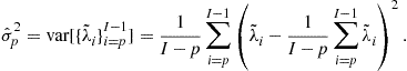 (21.15)
The number of components (for each mode) are selected using the following criterion:
![]() (21.16)
(21.16)
Recently, Ulfarsson and Solo [44] proposed an alternative more sophisticated method called SURE (Stein’s Unbiased Risk Estimator) which allows to estimate the number of PC components.
Extensive numerical experiments indicate that the Laplace method usually outperforms the BIC method while the GAP and SURE methods can often achieve significantly better performance than the Laplace method.
1.21.2.3 Whitening
Some adaptive algorithms for blind separation require prewhitening (also called sphering or normalized spatial decorrelation) of mixed (sensor) signals. A random, zero-mean vector ![]() is said to be white if its covariance matrix is an identity matrix, i.e.,
is said to be white if its covariance matrix is an identity matrix, i.e., ![]() or
or ![]() , where
, where ![]() is the Kronecker delta. In whitening, the sensor vectors
is the Kronecker delta. In whitening, the sensor vectors ![]() are pre-processed using the following transformation:
are pre-processed using the following transformation:
![]() (21.17)
(21.17)
Here ![]() denotes the whitened vector, and
denotes the whitened vector, and ![]() is an
is an ![]() whitening matrix. For
whitening matrix. For ![]() , where J is known in advance,
, where J is known in advance, ![]() simultaneously reduces the dimension of the data vectors from I to J. In whitening, the matrix
simultaneously reduces the dimension of the data vectors from I to J. In whitening, the matrix ![]() is chosen such that the scaled covariance matrix E
is chosen such that the scaled covariance matrix E![]() becomes the unit matrix
becomes the unit matrix ![]() . Thus, the components of the whitened vectors
. Thus, the components of the whitened vectors ![]() are mutually uncorrelated and have unit variance, i.e.,
are mutually uncorrelated and have unit variance, i.e.,
![]() (21.18)
(21.18)
Generally, the sensor signals are mutually correlated, i.e., the covariance matrix ![]() is a full (not diagonal) matrix. It should be noted that the matrix
is a full (not diagonal) matrix. It should be noted that the matrix ![]() is not unique, since multiplying it by an arbitrary orthogonal matrix from the left still preserves property (21.18). Since the covariance matrix of sensor signals
is not unique, since multiplying it by an arbitrary orthogonal matrix from the left still preserves property (21.18). Since the covariance matrix of sensor signals ![]() is symmetric positive semi-definite, it can be decomposed as follows:
is symmetric positive semi-definite, it can be decomposed as follows:
![]() (21.19)
(21.19)
where ![]() is an orthogonal matrix and
is an orthogonal matrix and ![]() is a diagonal matrix with positive eigenvalues
is a diagonal matrix with positive eigenvalues ![]() . Hence, under the condition that the covariance matrix is positive definite, the required decorrelation matrix
. Hence, under the condition that the covariance matrix is positive definite, the required decorrelation matrix ![]() (also called a whitening matrix or Mahalanobis transform) can be computed as follows:
(also called a whitening matrix or Mahalanobis transform) can be computed as follows:
![]() (21.20)
(21.20)
or
![]() (21.21)
(21.21)
where ![]() is an arbitrary orthogonal matrix. This can be easily verified by substituting (21.20) or (21.21) into (21.18):
is an arbitrary orthogonal matrix. This can be easily verified by substituting (21.20) or (21.21) into (21.18):
![]() (21.22)
(21.22)
or
![]() (21.23)
(21.23)
Alternatively, we can apply the Cholesky decomposition
![]() (21.24)
(21.24)
where ![]() is a lower triangular matrix. The whitening (decorrelation) matrix in this case is
is a lower triangular matrix. The whitening (decorrelation) matrix in this case is
![]() (21.25)
(21.25)
where ![]() is an arbitrary orthogonal matrix, since
is an arbitrary orthogonal matrix, since
![]() (21.26)
(21.26)
In the special case when ![]() is colored Gaussian noise with
is colored Gaussian noise with ![]() , the whitening transform converts it into a white noise (i.i.d.) process. If the covariance matrix is positive semi-definite, we can take only the positive eigenvalues and the associated eigenvectors.
, the whitening transform converts it into a white noise (i.i.d.) process. If the covariance matrix is positive semi-definite, we can take only the positive eigenvalues and the associated eigenvectors.
It should be noted that after pre-whitening of sensor signals ![]() , in the model
, in the model ![]() , the new mixing matrix defined as
, the new mixing matrix defined as ![]() is orthogonal (i.e.,
is orthogonal (i.e., ![]() ), if source signals are uncorrelated (i.e.,
), if source signals are uncorrelated (i.e., ![]() ), since we can write
), since we can write ![]() .
.
1.21.2.4 SVD
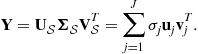
The Singular Value Decomposition (SVD) is a tool of both great practical and theoretical importance in signal processing and data analysis [40]. The SVD of a data matrix ![]() of rank-J with
of rank-J with ![]() , assuming without loss of generality that
, assuming without loss of generality that ![]() , leads to the following matrix factorization
, leads to the following matrix factorization
![]() (21.27)
(21.27)
where the matrix ![]() contains the T left singular vectors,
contains the T left singular vectors, ![]() has nonnegative elements on the main diagonal representing the singular values
has nonnegative elements on the main diagonal representing the singular values ![]() and the matrix
and the matrix ![]() represents the I right singular vectors called the loading factors. The nonnegative quantities
represents the I right singular vectors called the loading factors. The nonnegative quantities ![]() , sorted as
, sorted as ![]() can be shown to be the square roots of the eigenvalues of the symmetric matrix
can be shown to be the square roots of the eigenvalues of the symmetric matrix ![]() . The term
. The term ![]() is a
is a ![]() rank-1 matrix often called the jth eigenimage of
rank-1 matrix often called the jth eigenimage of ![]() . Orthogonality of the SVD expansion ensures that the left and right singular vectors are orthogonal, i.e.,
. Orthogonality of the SVD expansion ensures that the left and right singular vectors are orthogonal, i.e., ![]() and
and ![]() , with
, with ![]() the Kronecker delta (or equivalently
the Kronecker delta (or equivalently ![]() and
and ![]() ).
).
In many applications, it is more practical to work with the truncated form of the SVD, where only the first ![]() , (where J is the rank of
, (where J is the rank of ![]() , with
, with ![]() ) singular values are used, so that
) singular values are used, so that
 (21.28)
where ![]() and
and ![]() . This is no longer an exact decomposition of the data matrix
. This is no longer an exact decomposition of the data matrix ![]() , but according to the Eckart-Young theorem it is the best rank-P approximation in the least-squares sense and it is still unique (neglecting signs of vectors ambiguity) if the singular values are distinct.
, but according to the Eckart-Young theorem it is the best rank-P approximation in the least-squares sense and it is still unique (neglecting signs of vectors ambiguity) if the singular values are distinct.
For noiseless data, we can use the following decomposition:
 (21.29)
where ![]() and
and ![]() . The set of matrices
. The set of matrices ![]() represents this signal subspace and the set of matrices
represents this signal subspace and the set of matrices ![]() represents the null subspace or, in practice for noisy data, the noise subspace. The J columns of
represents the null subspace or, in practice for noisy data, the noise subspace. The J columns of ![]() , corresponding to these non-zero singular values that span the column space of
, corresponding to these non-zero singular values that span the column space of ![]() , are called the left singular vectors. Similarly, the J columns of
, are called the left singular vectors. Similarly, the J columns of ![]() are called the right singular vectors and they span the row space of
are called the right singular vectors and they span the row space of ![]() . Using these terms the SVD of
. Using these terms the SVD of ![]() can be written in a more compact form as:
can be written in a more compact form as:
 (21.30)
Perturbation theory for the SVD is partially based on the link between the SVD and the PCA and symmetric Eigenvalue Decomposition (EVD). It is evident, that from the SVD of the matrix ![]() with rank-
with rank-![]() , we have
, we have
![]() (21.31)
(21.31)
![]() (21.32)
(21.32)
where ![]() and
and ![]() . This means that the singular values of
. This means that the singular values of ![]() are the positive square roots of the eigenvalues of
are the positive square roots of the eigenvalues of ![]() and the eigenvectors
and the eigenvectors ![]() of
of ![]() are the left singular vectors of
are the left singular vectors of ![]() . Note that if
. Note that if ![]() , the matrix
, the matrix ![]() will contain at least
will contain at least ![]() additional eigenvalues that are not included as singular values of
additional eigenvalues that are not included as singular values of ![]() .
.
An estimate ![]() of the covariance matrix corresponding to a set of (zero-mean) observed vectors
of the covariance matrix corresponding to a set of (zero-mean) observed vectors ![]() may be computed as
may be computed as ![]() . An alternative equivalent way of computing
. An alternative equivalent way of computing ![]() is to form a data matrix
is to form a data matrix ![]() and represent the estimated covariance matrix by
and represent the estimated covariance matrix by ![]() . Hence, the eigenvectors of the sample covariance matrix
. Hence, the eigenvectors of the sample covariance matrix ![]() are the left singular vectors
are the left singular vectors ![]() of
of ![]() and the singular values
and the singular values ![]() of
of ![]() are the positive square roots of the eigenvalues of
are the positive square roots of the eigenvalues of ![]() .
.
From this discussion it follows that all the algorithms for PCA and EVD can be applied (after some simple tricks) to the SVD of an arbitrary matrix ![]() without any need to directly compute or estimate the covariance matrix. The opposite is also true; the PCA or EVD of the covariance matrix
without any need to directly compute or estimate the covariance matrix. The opposite is also true; the PCA or EVD of the covariance matrix ![]() can be performed via the SVD numerical algorithms. However, for large data matrices
can be performed via the SVD numerical algorithms. However, for large data matrices ![]() , the SVD algorithms usually become more costly, than the relatively efficient and fast PCA adaptive algorithms. Several reliable and efficient numerical algorithms for the SVD do however, exist [48].
, the SVD algorithms usually become more costly, than the relatively efficient and fast PCA adaptive algorithms. Several reliable and efficient numerical algorithms for the SVD do however, exist [48].
The approximation of the matrix ![]() by a rank-1 matrix
by a rank-1 matrix ![]() of two unknown vectors
of two unknown vectors ![]() and
and ![]() , normalized to unit length, with an unknown scaling constant term
, normalized to unit length, with an unknown scaling constant term ![]() , can be presented as follows:
, can be presented as follows:
![]() (21.33)
(21.33)
where ![]() is the matrix of the residual errors
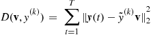
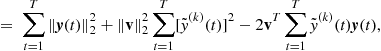
is the matrix of the residual errors ![]() . In order to compute the unknown vectors we minimize the squared Euclidean error as [49]
. In order to compute the unknown vectors we minimize the squared Euclidean error as [49]
 (21.34)
The necessary conditions for the minimization of (21.34) are obtained by equating the gradients to zero:
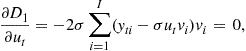 (21.35)
 (21.36)
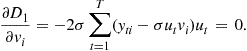
These equations can be expressed as follows:
 (21.37)
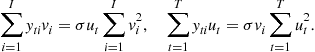
It is interesting to note that (taking into account that ![]() (see Eq. (21.37)) the cost function (21.34) can be expressed as [49]
(see Eq. (21.37)) the cost function (21.34) can be expressed as [49]
 (21.38)
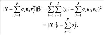
In matrix notation the cost function can be written as
![]() (21.39)
(21.39)
where the second term is called the Rayleigh quotient. The maximum value of the Rayleigh quotient is exactly equal to the maximum eigenvalue ![]() .
.
Taking into account that the vectors are normalized to unit length, that is, ![]() and
and ![]() , we can write the above equations in a compact matrix form as
, we can write the above equations in a compact matrix form as
![]() (21.40)
(21.40)
or equivalently (by substituting one of Eq. (21.40) into another)
![]() (21.41)
(21.41)
which are classical eigenvalue problems which estimate the maximum eigenvalue ![]() with the corresponding eigenvectors
with the corresponding eigenvectors ![]() and
and ![]() . The solutions of these problems give the best first rank-1 approximation of Eq. (21.27).
. The solutions of these problems give the best first rank-1 approximation of Eq. (21.27).
In order to estimate the next singular values and the corresponding singular vectors, we may apply a deflation approach, that is,
![]() (21.42)
(21.42)
where ![]() . Solving the same optimization problem (21.34) for the residual matrix
. Solving the same optimization problem (21.34) for the residual matrix ![]() yields the set of consecutive singular values and corresponding singular vectors. Repeating the reduction of the matrix yields the next set of solution until the deflation matrix
yields the set of consecutive singular values and corresponding singular vectors. Repeating the reduction of the matrix yields the next set of solution until the deflation matrix ![]() becomes zero. In the general case, we have:
becomes zero. In the general case, we have:
![]() (21.43)
(21.43)
Using the property of orthogonality of the eigenvectors and the equality ![]() , we can estimate the precision of the matrix approximation with the first
, we can estimate the precision of the matrix approximation with the first ![]() pairs of singular vectors [49]:
pairs of singular vectors [49]:
 (21.44)
and the residual error reduces exactly to zero when the number of singular values is equal to the matrix rank, that is, for ![]() . Thus, we can write for the rank-J matrix:
. Thus, we can write for the rank-J matrix:
 (21.45)
Note that the SVD can be formulated as the following constrained optimization problem:
![]() (21.46)
(21.46)
The cost function can be expressed as follows:
 (21.47)
Hence, for ![]() (with
(with ![]() and
and ![]() ) the problem (21.46) (called the best rank-1 approximation):
) the problem (21.46) (called the best rank-1 approximation):
![]() (21.48)
(21.48)
can be reformulated as an equivalent maximization problem (called the maximization variance approach):
![]() (21.49)
(21.49)
1.21.2.5 Very large-scale PCA/SVD
Suppose that ![]() is the SVD decomposition of an
is the SVD decomposition of an ![]() -dimensional matrix, where T is very large and I is moderate. Then matrices
-dimensional matrix, where T is very large and I is moderate. Then matrices ![]() and
and ![]() can be obtained form EDV/PCA decomposition of the
can be obtained form EDV/PCA decomposition of the ![]() -dimensional matrix
-dimensional matrix ![]() . The orthogonal matrix
. The orthogonal matrix ![]() can be then obtained from
can be then obtained from ![]() .
.
Remark
It should be noted that for moderate large-scale problems with ![]() and typically
and typically ![]() we can more efficiently solve the SVD problem by noting that the PCA/SVD of a semi-positive definite matrix (of much smaller dimension)
we can more efficiently solve the SVD problem by noting that the PCA/SVD of a semi-positive definite matrix (of much smaller dimension)
![]() (21.50)
(21.50)
with ![]() , has the same eigenvalues as the matrix
, has the same eigenvalues as the matrix ![]() , since we can write
, since we can write ![]() and
and ![]() and
and ![]() .
.
Moreover, if the vector ![]() is an eigenvector of the matrix
is an eigenvector of the matrix ![]() , then
, then ![]() is an eigenvector of
is an eigenvector of ![]() , since we can write
, since we can write
![]() (21.51)
(21.51)
In many practical applications dimension ![]() could be so large that the data matrix
could be so large that the data matrix ![]() can not be loaded into the memory of moderate class of computers. The simple solution is to partition of data matrix
can not be loaded into the memory of moderate class of computers. The simple solution is to partition of data matrix ![]() into, say, Q slices as
into, say, Q slices as ![]() , where the size of the qth slice
, where the size of the qth slice ![]() and can be optimized depending on the available computer memory [50,51]. The scaled covariance matrix (cross matrix product) can be then calculated as
and can be optimized depending on the available computer memory [50,51]. The scaled covariance matrix (cross matrix product) can be then calculated as
 (21.52)
since ![]() , where
, where ![]() are orthogonal matrices. Instead of computing the whole right singular matrix
are orthogonal matrices. Instead of computing the whole right singular matrix ![]() , we can perform calculations on the slices of the partitioned data matrix
, we can perform calculations on the slices of the partitioned data matrix ![]() as
as ![]() for
for ![]() . The concatenated slices
. The concatenated slices ![]() form the matrix of the right singular vectors
form the matrix of the right singular vectors ![]() . Such approach do not require loading the entire data matrix
. Such approach do not require loading the entire data matrix ![]() at once in the computer memory but instead use a sequential access to dataset. Of course, this method will work only if the dimension T is moderate, typically less than 10,000 and the dimension I can be theoretically arbitrary large.
at once in the computer memory but instead use a sequential access to dataset. Of course, this method will work only if the dimension T is moderate, typically less than 10,000 and the dimension I can be theoretically arbitrary large.
1.21.2.6 Basic algorithms for PCA/SVD
There are three basic or fundamental methods to compute PCA/SVD:
• The minimal reconstruction error approach:
 (21.53)
• The best rank-1 approximation approach:
![]() (21.54)
(21.54)
• The maximal variance approach:
![]() (21.55)
(21.55)
or in the more general form (for ![]() ):
):
![]() (21.56)
(21.56)
![]()
All the above approaches are connected or linked and almost equivalent. Often we impose additional constraints such as sparseness and/or nonnegativity (see Section 1.21.2.6.3).
1.21.2.6.1 Simple iterative algorithm using minimal reconstruction error approach
One of the simplest and intuitively understandable approaches to the derivation of adaptive algorithms for the extraction of true principal components without need to compute explicitly the covariance matrix is based on self-association (also called self-supervising or the replicator principle) [30,52]. According to this approach, we first compress the data vector ![]() to one variable
to one variable ![]() and next we attempt to reconstruct the original data from
and next we attempt to reconstruct the original data from ![]() by using the transformation
by using the transformation ![]() . Let us assume, that we wish to extract principal components (PCs) sequentially by employing the self-supervising principle (replicator) and a deflation procedure [30].
. Let us assume, that we wish to extract principal components (PCs) sequentially by employing the self-supervising principle (replicator) and a deflation procedure [30].
Let us consider a simple processing unit (see Figure 21.3)
 (21.57)
which extracts the first principal component, with ![]() . Strictly speaking, the factor
. Strictly speaking, the factor ![]() is called the first principal component of
is called the first principal component of ![]() , if the variance of
, if the variance of ![]() is maximally large under the constraint that the principal vector
is maximally large under the constraint that the principal vector ![]() has unit length.
has unit length.

The vector ![]() should be determined in such a way that the reconstruction vector
should be determined in such a way that the reconstruction vector ![]() will reproduce (reconstruct) the training vectors
will reproduce (reconstruct) the training vectors ![]() as correctly as possible, according to the following cost function
as correctly as possible, according to the following cost function ![]() , where
, where ![]() . In general, the loss (cost) function is expressed as
. In general, the loss (cost) function is expressed as
 (21.58)
where
![]()
In order to increase the convergence speed, we can minimize the cost function (21.58) by employing the cascade recursive least-squares (CRLS) approach for optimal updating of the learning rate ![]() [52,53]:
[52,53]:
![]() (21.59)
(21.59)
![]() (21.60)
(21.60)
![]() (21.61)
(21.61)
 (21.62)
![]() (21.63)
(21.63)
![]() (21.64)
(21.64)
where ![]() denotes the vector
denotes the vector ![]() after achieving convergence. The above algorithm is fast and accurate for extracting sequentially an arbitrary number of eigenvectors in PCA.
after achieving convergence. The above algorithm is fast and accurate for extracting sequentially an arbitrary number of eigenvectors in PCA.
1.21.2.6.2 Power methods for standard PCA
Many iterative algorithms for PCA exploit the Rayleigh quotient (RQ) of the specific covariance matrix as the cost function and power methods [54,55]. The Rayleigh quotient ![]() is defined for
is defined for ![]() , as
, as
![]() (21.65)
(21.65)
It is worth to note that
![]() (21.66)
(21.66)
where ![]() and
and ![]() denote the largest and the smallest eigenvalues of the covariance matrix
denote the largest and the smallest eigenvalues of the covariance matrix ![]() , respectively.
, respectively.
More generally, the critical points and critical values of ![]() are the eigenvectors and eigenvalues of
are the eigenvectors and eigenvalues of ![]() . Assuming that the eigenvalues of the covariance matrix can be ordered as
. Assuming that the eigenvalues of the covariance matrix can be ordered as ![]() , and that the principal eigenvector
, and that the principal eigenvector ![]() has unit length, i.e.,
has unit length, i.e., ![]() , we can estimate it using the following iterations
, we can estimate it using the following iterations
![]() (21.67)
(21.67)
Taking into account that ![]() and
and ![]() , we can then use the following simplified formula
, we can then use the following simplified formula
![]() (21.68)
(21.68)
or more generally, for a number of higher PCs, we may use the deflation approach as
 (21.69)
where ![]() . After the convergence of the vector
. After the convergence of the vector ![]() to
to ![]() , we perform the deflation as:
, we perform the deflation as: ![]() .
.
The above fast PCA algorithm can be derived also in a slightly modified form by minimizing the cost function:
 (21.70)
subject to the constraint ![]() . The cost function achieves equilibrium when the gradient of D is zero, i.e.,
. The cost function achieves equilibrium when the gradient of D is zero, i.e.,
 (21.71)
This suggests the following iteration formula [55,56]:
 (21.72)
Remark
It should be noted that the convergence rate of the power algorithm depends on a ratio ![]() , where
, where ![]() is the second largest eigenvalue of
is the second largest eigenvalue of ![]() . This ratio is generally smaller than one, allowing adequate convergence of the algorithm. However, if the eigenvalue
. This ratio is generally smaller than one, allowing adequate convergence of the algorithm. However, if the eigenvalue ![]() has one or more other eigenvalues of
has one or more other eigenvalues of ![]() close by, in other words, when
close by, in other words, when ![]() belongs to a cluster of eigenvalues then the ratio can be very close to one, causing very slow convergence, and as a consequence, the estimated eigenvector
belongs to a cluster of eigenvalues then the ratio can be very close to one, causing very slow convergence, and as a consequence, the estimated eigenvector ![]() may be inaccurate for noisy data or collinear components. For multiple eigenvalues, the power method will fail to converge.
may be inaccurate for noisy data or collinear components. For multiple eigenvalues, the power method will fail to converge.
1.21.2.6.3 Extensions of standard PCA
1.21.2.6.3.1 Sparse PCA
The importance of the standard PCA is mainly due to the following three important properties:
1. The principal components sequentially capture the maximum variability (variance) of the data matrix ![]() , thus guaranteeing minimal information loss in the sense of mean squared errors.
, thus guaranteeing minimal information loss in the sense of mean squared errors.
2. The principal components are uncorrelated, i.e., ![]() .
.
3. The PCs are hierarchically organized with the respect to decreasing values of their variances (eigenvalues of the covariance matrix).
The standard PCA/SVD has also several disadvantages, especially for large-scale and noisy problems. A particular disadvantage that the standard principal components ![]() are usually a linear combination of all the variables
are usually a linear combination of all the variables ![]() . In other words, all weights
. In other words, all weights ![]() (referred as loadings) are not zero. This means that the principal vectors
(referred as loadings) are not zero. This means that the principal vectors ![]() are dense (not sparse) what makes often the physical interpretation of the principal components difficult in many applications. For example, in many applications (from biology to image understanding) the coordinate axes have a physical interpretations (each axis might correspond to a specific feature), but only if the components are sparsely represented, i.e., by a very few non zero loadings (coordinates). Recently several modifications of PCA have been proposed which impose some sparseness for the principal (basis) vectors and corresponding components are called sparse principal components [54,57–62]. The main idea in SPCA is to force the basis vectors to be sparse, however the sparsity profile should be adjustable or well controlled via some parameters in order to discover specific features in the observed data. In other words, our objective is to estimate sparse principal components, i.e., the sets of sparse vectors
are dense (not sparse) what makes often the physical interpretation of the principal components difficult in many applications. For example, in many applications (from biology to image understanding) the coordinate axes have a physical interpretations (each axis might correspond to a specific feature), but only if the components are sparsely represented, i.e., by a very few non zero loadings (coordinates). Recently several modifications of PCA have been proposed which impose some sparseness for the principal (basis) vectors and corresponding components are called sparse principal components [54,57–62]. The main idea in SPCA is to force the basis vectors to be sparse, however the sparsity profile should be adjustable or well controlled via some parameters in order to discover specific features in the observed data. In other words, our objective is to estimate sparse principal components, i.e., the sets of sparse vectors ![]() spanning a low-dimensional space that represent most of the variance present in the data
spanning a low-dimensional space that represent most of the variance present in the data ![]() .
.
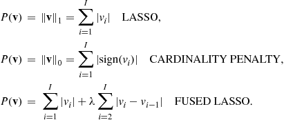
Many methods have been proposed for estimating sparse principal components, based on either the maximum-variance property of the principal components, or on the regression/reconstruction error property. The most important approaches which extract the principal eigenvectors sequentially can be summarized as the following constrained or penalized optimization problems [54,57,59–63]:
1. ![]() -norm constrained SPCA or the SCoTLASS procedure [59] uses the maximal variance characterization for the principal components. The first sparse principal component solves the optimization problem:
-norm constrained SPCA or the SCoTLASS procedure [59] uses the maximal variance characterization for the principal components. The first sparse principal component solves the optimization problem:
![]() (21.73)
(21.73)
and subsequent components solve the same problem but with the additional constraint that they must be orthogonal to the previous components. When the parameter ![]() is sufficiently large, then the optimization problem (21.73) simply yields the first standard principal component of
is sufficiently large, then the optimization problem (21.73) simply yields the first standard principal component of ![]() , and when
, and when ![]() is small, then the solution is sparse.
is small, then the solution is sparse.
2. ![]() -norm penalized SPCA [64]
-norm penalized SPCA [64]
![]() (21.74)
(21.74)
where the penalty parameter ![]() controls the level of sparseness.
controls the level of sparseness.
3. ![]() -norm penalized SPCA [57]
-norm penalized SPCA [57]
![]() (21.75)
(21.75)
4. SPCA using Penalized Matrix decomposition (PMD) [61,64]
![]() (21.76)
(21.76)
where positive parameters ![]() control sparsity level and the convex penalty functions
control sparsity level and the convex penalty functions ![]() and
and ![]() can take a variety of different forms. Useful examples are:
can take a variety of different forms. Useful examples are:
5. SPCA via regularized SVD (sPCA-rSVD) [54,65]
![]() (21.77)
(21.77)
6. Two-way functional PCA/SVD [66]
![]() (21.78)
(21.78)
7. Sparse SVD [67]
![]() (21.79)
(21.79)
8. Generalized SPCA [68]
![]() (21.80)
(21.80)
where ![]() and
and ![]() are symmetric positive definite matrices.
are symmetric positive definite matrices.
9. Generalized nonnegative SPCA [63]
![]() (21.81)
(21.81)
10. Robust SPCA [69]
![]() (21.82)
(21.82)
where ![]() are multivariate observations collected in the rows of the data matrix
are multivariate observations collected in the rows of the data matrix ![]() and Var is a robust variance measure.
and Var is a robust variance measure.
There exist some connections between the above listed optimizations problems, and in fact they often deliver almost identical or at least similar solutions. All the optimization problems addressed here are rather difficult, generally non-convex maximization problems, and we can not make a claim with respect their global optimality. Even if the goal of obtaining a local minimizer is, in general, unattainable we must be content with convergence to a stationary point. However, using so formulated optimization problems, the common and interesting feature of the resulting algorithms is, that they provide a closed-form iterative updates (which is a generalized power method):
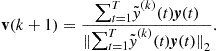
![]() (21.83)
(21.83)
or
![]() (21.84)
(21.84)
where ![]() is a simple operator (shrinkage) which can be written in explicit form and can be efficiently computed [54,60].
is a simple operator (shrinkage) which can be written in explicit form and can be efficiently computed [54,60].
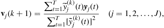
For example, by applying the optimization problem (21.77) we obtain the sparse SVD algorithm. Sparse SVD can be performed by solving the following optimization problem:
![]() (21.85)
(21.85)
![]() (21.86)
(21.86)
which leads to the following update formulas:
![]() (21.87)
(21.87)
where the non-negative parameters ![]() control sparsity level and the operator
control sparsity level and the operator ![]() means the shrinkage function defined as
means the shrinkage function defined as
![]() (21.88)
(21.88)
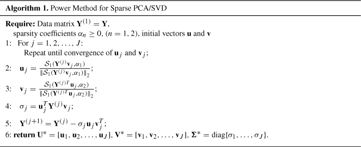
In fact, when ![]() is the identity operator, the above update schemes are nothing else but power method for the standard PCA/SVD (see Algorithm 1).
is the identity operator, the above update schemes are nothing else but power method for the standard PCA/SVD (see Algorithm 1).
In contrast to standard PCA, SPCA enables to reveal often multi-scale hierarchical structures from the data [62]. For example, for EEG data the SPCA generates spatially localized, narrow bandpass functions as basis vectors, thereby achieving a joint space and frequency representation, what is impossible to obtain by using standard PCA. The algorithm for sparse PCA/SVD can be easily extended to sparse CCA/PLS (see Section 1.21.2.6.6).
1.21.2.6.4 Deflation techniques for SPCA
In sparse PCA the eigenvectors are not necessary mutually orthogonal. In fact, we usually alleviate or even completely ignore the orthogonality constraints. Due to this reason the standard Hotelling deflation procedure:
![]() (21.89)
(21.89)
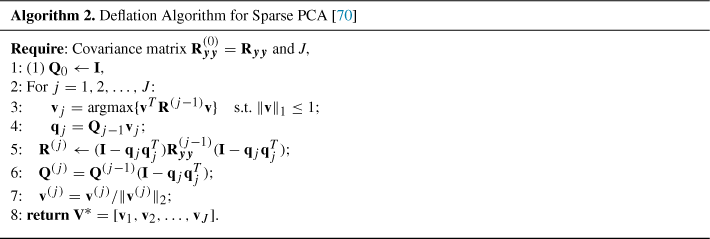
does not guarantee the positive semi-definiteness of the covariance matrix. Due to this reason we usually use the Schur compliment deflation [70]:
![]() (21.90)
(21.90)
or alternatively the projection deflation
![]() (21.91)
(21.91)
Empirical studies by Mackey [70] indicate that the Schur deflation and the projection deflation outperform the standard Hotelling’s deflation consistently for SPCA, and usually the projection deflation is even better than (or at least comparable with) the Schur deflation.
1.21.2.6.5 Kernel PCA
Standard PCA applies linear transformation for dimensionality reduction and may not be effective for nonlinear data. In kernel PCA we apply implicitly nonlinear transformation to potentially very high dimensional feature space ![]() .
.
Let consider a data matrix ![]() with vectors
with vectors ![]() (typically, with
(typically, with ![]() ), which are nonlinearly projected feature subspace
), which are nonlinearly projected feature subspace
![]() (21.92)
(21.92)
The covariance matrix in the feature space can be expressed as
 (21.93)
where ![]() (we assume without loos of generality that
(we assume without loos of generality that ![]() ). However, in practice, we almost never compute the nonlinear mapping
). However, in practice, we almost never compute the nonlinear mapping ![]() explicitly, since the feature space can be very high dimensional in the kernel method, but rather exploit so called “kernel trick”, i.e., employ the nonlinear mapping implicitly [71].
explicitly, since the feature space can be very high dimensional in the kernel method, but rather exploit so called “kernel trick”, i.e., employ the nonlinear mapping implicitly [71].
Let ![]() be eigenvector of the covariance matrix
be eigenvector of the covariance matrix ![]() , then the vector
, then the vector ![]() belongs to linear space spanned by the data points
belongs to linear space spanned by the data points ![]() (
(![]() ) since
) since ![]() implies that
implies that ![]() . So, the standard PCA can be formulated in dual form as
. So, the standard PCA can be formulated in dual form as ![]() , where
, where ![]() is referred to as linear kernel matrix with entries
is referred to as linear kernel matrix with entries ![]() expressed by inner products.
expressed by inner products.
Similarly, eigenvector ![]() of the covariance matrix
of the covariance matrix ![]() defined by Eq. (21.93) can be written as
defined by Eq. (21.93) can be written as ![]() . Taking into account that
. Taking into account that
![]() (21.94)
(21.94)
 (21.95)
By multiplying the both side of the above equation by ![]() , we obtain
, we obtain
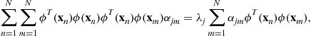 (21.96)
which can be written in a compact matrix form as ![]() or equivalently
or equivalently
![]() (21.97)
(21.97)
where ![]() is a kernel positive definite symmetric matrix with entries defined as
is a kernel positive definite symmetric matrix with entries defined as ![]() . We can estimate the kernel PCA features for new sample as
. We can estimate the kernel PCA features for new sample as
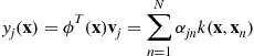 (21.98)
Summarizing, the Kernel PCA algorithm can be formulated as follows:
1. Step 1: Select kernel function (e.g., Gaussian kernel: ![]() or polynomial kernel:
or polynomial kernel: ![]() ) and compute the kernel matrix with entries
) and compute the kernel matrix with entries ![]() (
(![]() ) for training set.
) for training set.
2. Step 2: Compute eigenvalues and eigenvectors pairs of ![]() as
as ![]() .
.
3. Step 3: Normalize the eigenvectors ![]() .
.
4. Step 4: To project a test feature ![]() onto
onto ![]() we need to compute
we need to compute ![]() . So, explicit nonlinear mapping
. So, explicit nonlinear mapping ![]() is not required here.
is not required here.
1.21.2.6.6 Sparse CCA
The Canonical Correlation Analysis (CCA), introduced by Hotelling [72], can be considered as a generalization or extension of PCA (see [73,74]. The standard CCA is a classical method for determining the relationship between two sets of variables. Given two zero-mean (i.e., centered) data sets ![]() and
and ![]() on the same set of I observations, CCA seeks linear combinations of the variables in
on the same set of I observations, CCA seeks linear combinations of the variables in ![]() and the variables in
and the variables in ![]() that are maximally correlated with each other. Formally, the classical CCA computes two projection vectors
that are maximally correlated with each other. Formally, the classical CCA computes two projection vectors ![]() and
and ![]() such that the correlation coefficient
such that the correlation coefficient
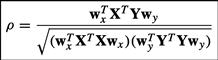 (21.99)
In a similar way, we can formulate a kernel CCA by replacing inner product matrices by kernel matrices:
 (21.100)
where ![]() and
and ![]() are suitably designed kernel matrices. The above optimization problem can be solved by generalized eigenvalue decomposition.
are suitably designed kernel matrices. The above optimization problem can be solved by generalized eigenvalue decomposition.
Since ![]() is invariant to the scaling of the vectors
is invariant to the scaling of the vectors ![]() and
and ![]() , the standard CCA can be formulated equivalently as the following constrained optimization problem:
, the standard CCA can be formulated equivalently as the following constrained optimization problem:
![]() (21.101)
(21.101)
We will refer to ![]() and
and ![]() as the canonical variables.
as the canonical variables.
For sparse CCA we usually assume that the columns of ![]() and
and ![]() have been standardized to have mean zero and standard deviation one.
have been standardized to have mean zero and standard deviation one.
In order to obtain sparse CCA we must impose suitable sparsity constraints on the canonical vectors, for example by applying the PMD approach [61,64]:
![]() (21.102)
(21.102)
where ![]() and
and ![]() are convex penalty functions and positive parameters
are convex penalty functions and positive parameters ![]() control sparsity level (see Section 1.21.2.6.3). Since
control sparsity level (see Section 1.21.2.6.3). Since ![]() and
and ![]() are generally chosen to yield sparse canonical vectors
are generally chosen to yield sparse canonical vectors ![]() and
and ![]() , we call this criterion the sparse CCA.
, we call this criterion the sparse CCA.
Note that since the data are standardized, cross product matrices ![]() and
and ![]() are approximated by identity matrices, and consequently the constraints
are approximated by identity matrices, and consequently the constraints ![]() and
and ![]() may be replaced by
may be replaced by ![]() and
and ![]() , respectively [64].
, respectively [64].
The algorithms for the sparse CCA will be similar to sparse SVD/PCA (see Algorithm 3) in which the data matrix ![]() in the SPCA should be replaced by
in the SPCA should be replaced by ![]() in the SCCA and the vectors
in the SCCA and the vectors ![]() and
and ![]() by the vectors
by the vectors ![]() and
and ![]() , respectively.
, respectively.
In order to compute multiple canonical vectors for CCA we need to apply a suitable deflation in a similar way as for SPCA. For example, we can compute the vectors ![]() and
and ![]() for
for ![]() by applying criterion (21.102) to the data sets:
by applying criterion (21.102) to the data sets:
![]() (21.103)
(21.103)
Note that the deflation and generalized power method do not impose automatically orthogonality constraints vectors ![]() and
and ![]() . In order to enforce orthogonality for the subsequently computed on the vectors
. In order to enforce orthogonality for the subsequently computed on the vectors ![]() , we can apply the Gram-Schmidt orthogonalization method [68]:
, we can apply the Gram-Schmidt orthogonalization method [68]:
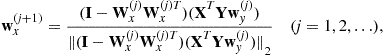 (21.104)
1.21.2.6.7 Sparse partial least squares
The Partial Least Squares (PLS) methods, originally developed in chemometrics and econometrics by Herman Wold and his coworkers (see [75] and references therein) are particularly suitable for the analysis of relationships among multi-modal brain data (e.g., EEG, MEG, ECoG (electrocorticogram), fMRI) or relationships between measures of brain activity and behavior data [76,77]. The standard PLS approaches have been recently summarized in [75,78] and their suitability to model relationships between brain activity and behavior (experimental design) has been highlighted in [76].
There are two related basic PLS methods: PLS correlation (PLSC), which analyzes correlations or (associations) between two or more sets of data (e.g., two modalities brain data or brain and behavior data) and PLS regression (PLSR) methods, which attempt to predict one set of data from another independent set of data that constitutes the predictors (e.g., predict experimental behavior data from brain data such as multichannel ECoG or scalp EEG from ECoG by performing simultaneous recordings for epileptic patients).
In order to predict the response variables represented by the matrix ![]() from the independent variables
from the independent variables ![]() , the standard PLSR techniques find a set of common orthogonal latent variables (also called latent vectors, score vectors or components) by projecting both
, the standard PLSR techniques find a set of common orthogonal latent variables (also called latent vectors, score vectors or components) by projecting both ![]() and
and ![]() onto a subspace, which ensures a maximal covariance between the latent variables of
onto a subspace, which ensures a maximal covariance between the latent variables of ![]() and
and ![]() . In other words, the prediction is achieved by simultaneous approximative decompositions training data sets:
. In other words, the prediction is achieved by simultaneous approximative decompositions training data sets: ![]() and
and ![]() into factor matrices (components) (
into factor matrices (components) (![]() and
and ![]() ), respectively:
), respectively:
![]() (21.105)
(21.105)
![]() (21.106)
(21.106)
with the constraint that these components explain as much as possible of the covariance between ![]() and
and ![]() [64,77]. In other words, the key concept of basic PLS algorithms is to maximize covariance between the vectors
[64,77]. In other words, the key concept of basic PLS algorithms is to maximize covariance between the vectors ![]() and
and ![]() expressed in a general form as:
expressed in a general form as:
![]() (21.107)
(21.107)
subject to suitable constraints, where the function ![]() may take different forms: the identity, the absolute value or the square function, and we define the vectors as
may take different forms: the identity, the absolute value or the square function, and we define the vectors as ![]() and
and ![]() .
.
More generally, the objective of the standard PLS is to find in the first step directions defined by ![]() and
and ![]() that maximize the set of cost functions (see Figure 21.4):
that maximize the set of cost functions (see Figure 21.4):
![]() (21.108)
(21.108)
![]()
In other words, the basic approach to the standard PLS is to find these direction vectors ![]() and
and ![]() from successive optimizations problems (see also Eq. (21.102)). The latent components can be defined as
from successive optimizations problems (see also Eq. (21.102)). The latent components can be defined as ![]() and
and ![]() , or equivalently
, or equivalently ![]() and
and ![]() for
for ![]() .
.
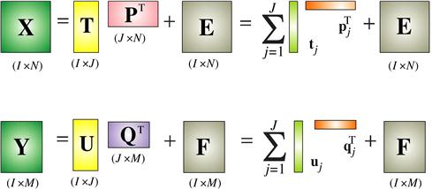
Figure 21.4 Illustration of a basic PLS model. In this model ![]() is a matrix of predictors,
is a matrix of predictors, ![]() is the response matrix,
is the response matrix, ![]() and
and ![]() are loading matrices for the predictor and response with corresponding
are loading matrices for the predictor and response with corresponding ![]() and
and ![]() component matrices, and matrices
component matrices, and matrices ![]() and
and ![]() are corresponding error terms. Our objective is to perform approximative decompositions of the matrices X and Y and by imposing additional orthogonality and optional sparsity constraints.
are corresponding error terms. Our objective is to perform approximative decompositions of the matrices X and Y and by imposing additional orthogonality and optional sparsity constraints.
The main difference between PLS and CCA is that the CCA maximize the correlation while the PLS maximize the covariance. Moreover, in the PLS the primary objective is to estimate matrices ![]() and
and ![]() while in the CCA we estimate only projection matrices
while in the CCA we estimate only projection matrices ![]() and
and ![]() . Anyway, the PLS and CCA are quite similar for the standardized data (that is after the columns of
. Anyway, the PLS and CCA are quite similar for the standardized data (that is after the columns of ![]() and
and ![]() have been standardized to have mean zero and standard deviation) one the both method are equivalent.
have been standardized to have mean zero and standard deviation) one the both method are equivalent.
The PLS decomposition allows us to find relationships between the components which can be used to predict the values of the dependent variables ![]() for new situations, if the values of the corresponding independent variables
for new situations, if the values of the corresponding independent variables ![]() are available:
are available:
![]() (21.109)
(21.109)
The predictive relationship between the two sets of data is driven by a linear regression model involving J pairs of latent variables: ![]() , (or in a matrix form
, (or in a matrix form ![]() ), where
), where ![]() is a scaling regression coefficient and
is a scaling regression coefficient and ![]() represents residual errors [79]. Using this basic inner regression model the standard PLS model can be expressed as
represents residual errors [79]. Using this basic inner regression model the standard PLS model can be expressed as
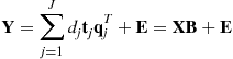 (21.110)
where the regression coefficients matrix has been defined as ![]() .
.
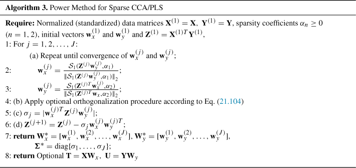
Assuming that the vectors component matrices are estimated sequentially (using deflation approach), the loading factors and regression coefficient can be calculated as:
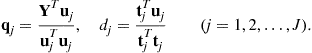 (21.111)
Often, we impose additional (optional) sparseness and/or orthogonality constraints (imposed on components matrices ![]() and
and ![]() or the loading matrices), in order to achieve better predictive power. For high dimensional data sets, it is often appropriate to assume that independent and dependent data has unit covariance matrices, i.e.,
or the loading matrices), in order to achieve better predictive power. For high dimensional data sets, it is often appropriate to assume that independent and dependent data has unit covariance matrices, i.e., ![]() and
and ![]() . In the case of the sparse PLS, we can formulate as the following optimization problem
. In the case of the sparse PLS, we can formulate as the following optimization problem
![]() (21.112)
(21.112)
![]()
The PLS algorithms have been proven to be particularly powerful for strongly collinear data and for underdetermined independent data (i.e., more variables than observations) [77]. The widely reported sensitivity to noise of the PLS regression is attributed to redundant (irrelevant) latent variables, their selection remains an open problem. Other problems include the difficulty of interpreting the loadings corresponding to the latent variables, and the fact that the number of latent variables cannot exceed the minimum number of predictors and observations.
Sparse PCA, CCA, and PLS deliver components (or latent vectors) that can be considered as a compromise between maximizing the variance, correlation or covariance, respectively and improving the interpretability of the data, especially for large-scale data with possibly fewer observations than variables. The extraction of components and latent variables sequentially, one by one, by applying deflation techniques, allows us to stop the algorithms after achieving the desired number of components and/or achieving an error measure below a specified threshold.
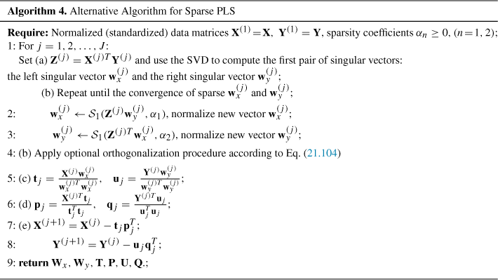
1.21.3 ICA and related problems
There are at least three basic approaches for ICA, coming from different models of source signals [13,14,17]. The first simple model considers weakly stationary Gaussian processes and exploits directly the second order statistics (SOS). These signals are separable if their spectra are distinct; therefore, the separation is based on the spectral diversity of the sources. The second approach takes the nonstationarity of the signals into account by modeling them as independently distributed Gaussian variables whose variance is changing in time. For the third basic approach one assumes that source signals are represented by sequence of identically and independently distributed random variables. The condition of separability of such source signals requires that at most only one signal is Gaussian, so the approach is said to be based on the non-Gaussianity and it exploits higher order statistics (HOS). Strictly speaking the first two approaches do not explicitly or implicitly assume statistical independence but rather generalized decorrelation via simultaneous joint diagonalization of time-delayed covariance matrices.
Spatial decorrelation (or prewhitening) is often considered a necessary (but not sufficient) condition for stronger stochastic independence criteria. After prewhitening ICA tasks usually become somewhat easier and well-posed (or less ill-conditioned), because the subsequent separating (unmixing) system is described by an orthogonal matrix for real-valued signals and by a unitary matrix for complex-valued signals and weights. Furthermore, the spatio-temporal and time-delayed decorrelation can be used to identify the mixing matrix and to perform blind source separation of colored sources under certain weak conditions [13,14,17,18,80]. Temporal, spatial and spatio-temporal decorrelations play important roles in EEG/MEG data analysis. These techniques are based only on second-order statistics (SOS). They are the basis for modern subspace methods of spectrum analysis and array processing and are often used in a preprocessing stage in order to improve the convergence properties of adaptive systems, to eliminate redundancy or to reduce noise. Spatio-temporal data has both spatial (i.e., location) and temporal (i.e., time related) components.
One possible extension of the ICA is the so-called Independent Subspace Analysis (ISA). ISA can be applied to situations where not all source signals can be separated from each other by linear transformations. The goal here is to decompose the linear space spanned by rows of Y to a direct (orthogonal) sum of linear subspaces, such that elements of each subspace are statistically independent of the others. The ISA problem can be approached by applying an ICA algorithm, which aims to separate each component from the others as much as possible. In the postprocessing step we usually perform clustering of the obtained components according to their residual mutual dependence.
1.21.3.1 The AMUSE algorithm and its properties
AMUSE (Algorithm for Multiple Unknown Signal Extraction) is probably the simplest BSS algorithm which belongs to the group of Second-Order Statistics Spatio-Temporal Decorrelation (SOS-STD) algorithms [14,81]. It provides similar decompositions for noiseless data to the well known and popular SOBI and TDSEP algorithms [82,83]. This class of algorithms are sometimes classified or referred to as ICA algorithms. However, these algorithms do not exploit implicitly or explicitly the statistical independence. Moreover, in contrast to standard higher order statistics ICA algorithms, they are able to estimate colored Gaussian distributed sources and their performance in estimation of original sources is usually better if the sources have temporal structures.
The AMUSE algorithm has some similarity with the standard PCA. The main difference is that the AMUSE employs PCA two times in two separate steps: In the first step, standard PCA is applied for the whitening (sphering) of the data and in the second step PCA is applied to the time delayed covariance matrix of the pre-whitened data. Mathematically the AMUSE algorithm consists of the following two stage procedure: In the first step we apply standard or robust prewhitening as a linear transformation ![]() , where
, where ![]() of the standard covariance matrix
of the standard covariance matrix ![]() , and
, and ![]() is a vector of observed data for time point t. Next, (for the pre-whitened data) the SVD is applied for the time-delayed covariance matrix
is a vector of observed data for time point t. Next, (for the pre-whitened data) the SVD is applied for the time-delayed covariance matrix ![]() (typically, with
(typically, with ![]() ), where
), where ![]() is a diagonal matrix with decreasing singular values and
is a diagonal matrix with decreasing singular values and ![]() are orthogonal matrices containing the of left and right singular vectors. Then, an unmixing (separating) matrix is estimated as
are orthogonal matrices containing the of left and right singular vectors. Then, an unmixing (separating) matrix is estimated as ![]() .
.
The main advantages of the AMUSE algorithm over the other BSS/ICA algorithms is its simplicity and that it allows the automatic ordering of the components, due to application of SVD. In fact, the components are ordered according to the decreasing values of the singular values of the time-delayed covariance matrix. In other words, the AMUSE algorithm exploits the simple principle that the estimated components tends to be less complex or more precisely that they have better linear predictability than any mixture of those sources. It should be emphasized that all components estimated by AMUSE are uniquely defined and consistently ranked. The consistent ranking is due to the fact that these singular values are always ordered in decreasing values. For real-world data probability that two singular values achieve exactly the same value is very small, so ordering is consistent and unique [14]. The one disadvantage of the AMUSE algorithm it is that is very sensitive to additive noise since the algorithm exploits only one time delayed covariance matrix.
1.21.3.2 The SOBI algorithm and its extensions
The second-order blind identification (SOBI) algorithm is a classical blind source separation (BSS) algorithm for wide-sense stationary (WSS) processes with distinct spectra [82]. This algorithm has proven to be very useful in biomedical applications and it has became more popular than the other algorithms.
There is a common practice in ICA/BSS research to exploit the “average eigen-structure” of a large set of data matrices formed as functions of the available data (typically, covariance or cumulant matrices for different time delays). In other words, the objective is to extract reliable information (e.g., estimation of sources and/or of the mixing matrix) from the eigen-structure of a possibly large set of data matrices [14,82,84,85]. However, since in practice we only have a finite number of samples of signals corrupted by noise, the data matrices do not exactly share the same eigen-structure. Furthermore, it should be noted that determining the eigen-structure on the basis of one or even two data matrices usually leads to poor or unsatisfactory results, because such matrices, based usually on an arbitrary choice, may have degenerate eigenvalues leading to loss of the information contained in other data matrices. Therefore, from a statistical point of view, in order to provide robustness and accuracy, it is necessary to consider the average eigen-structure by taking into account simultaneously a possibly large set of data matrices [14,85].
The average eigen-structure can be easily implemented via the linear combination of several time-delayed covariance matrices and by applying the standard EVD or SVD. An alternative approach to EVD/SVD is to apply the approximate joint diagonalization procedure (JAD). The objective of this procedure is to find the orthogonal matrix ![]() which diagonalizes a set of matrices [82,84,85]:
which diagonalizes a set of matrices [82,84,85]:
![]() (21.113)
(21.113)
where ![]() are data matrices (for example, time-delayed covariance matrices), the
are data matrices (for example, time-delayed covariance matrices), the ![]() are diagonal and real, and
are diagonal and real, and ![]() represent additive errors (as small as possible). If
represent additive errors (as small as possible). If ![]() for arbitrary matrices
for arbitrary matrices ![]() , the problem becomes overdetermined and generally we can not find an exact diagonalizing matrix
, the problem becomes overdetermined and generally we can not find an exact diagonalizing matrix ![]() with
with ![]() . An important advantage of the Joint Approximate Diagonalization (JAD) is that several numerically efficient algorithms exist for its computation, including Jacobi techniques (one sided and two sided), Alternating Least Squares (ALS), PARAFAC (Parallel Factor Analysis) and subspace fitting techniques employing the efficient Gauss–Newton optimization [85]. This idea has been implemented as a robust SOBI algorithm which can be briefly outlined as follows [14,86]:
. An important advantage of the Joint Approximate Diagonalization (JAD) is that several numerically efficient algorithms exist for its computation, including Jacobi techniques (one sided and two sided), Alternating Least Squares (ALS), PARAFAC (Parallel Factor Analysis) and subspace fitting techniques employing the efficient Gauss–Newton optimization [85]. This idea has been implemented as a robust SOBI algorithm which can be briefly outlined as follows [14,86]:
1. Perform robust orthogonalization ![]() , similar as to the AMUSE algorithm.
, similar as to the AMUSE algorithm.
2. Estimate the set of covariance matrices:
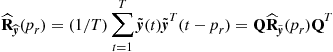 (21.114)
for a preselected set of time lags (![]() ) or bandpass filters
) or bandpass filters ![]() .
.
3. Perform JAD: ![]() , i.e., estimate the orthogonal matrix
, i.e., estimate the orthogonal matrix ![]() using one of the available numerical algorithms.
using one of the available numerical algorithms.
4. Estimate the source signals as ![]() , and then the mixing matrix as
, and then the mixing matrix as ![]() .
.
The main advantage of the SOBI algorithm is its robustness with respect to additive noise if number of covariance matrices is sufficiently large (typically, ![]() ).
).
Several extensions and modifications of the SOBI algorithm have been proposed, e.g., Robust SOBI [14], thinICA [87], and WASOBI [88,89] (the weights-adjusted variant of SOBI), which is asymptotically optimal (in separating Gaussian parametric processes). The WASOBI for the separation of independent stationary sources is modeled as Auto-Regressive (AR) random processes. The matrices are computed for the case of Gaussian sources, for which the resulting separation would be asymptotically optimal approaching the corresponding Cramer-Rao bound (CRB) for the best possible separation [88,90].
1.21.3.3 ICA based on higher order statistics (HOS)
The ICA of a random vector ![]() can be performed by finding an
can be performed by finding an ![]() , (with
, (with ![]() ), full rank separating (transformation) matrix
), full rank separating (transformation) matrix ![]() , such that the output signal vector
, such that the output signal vector ![]() (components) estimated by
(components) estimated by
![]() (21.115)
(21.115)
are as independent as possible as evaluated by an information-theoretic cost function such as the minimum of the Kullback-Leibler divergence [14,17,91,92].
The statistical independence of random variables is a more general concept than decorrelation. Roughly speaking, we say that the random variables ![]() and
and ![]() are statistically independent if knowledge of the value of
are statistically independent if knowledge of the value of ![]() provides no information about the values of
provides no information about the values of ![]() . Mathematically, the independence of
. Mathematically, the independence of ![]() and
and ![]() can be expressed by the relationship
can be expressed by the relationship
![]() (21.116)
(21.116)
where ![]() denotes the probability density function (pdf) of the random variable x. In other words, signals are independent if their joint pdf can be factorized.
denotes the probability density function (pdf) of the random variable x. In other words, signals are independent if their joint pdf can be factorized.
If independent signals are zero-mean, then the generalized covariance matrix of ![]() and
and ![]() , where
, where ![]() and
and ![]() are different, odd nonlinear activation functions (e.g.,
are different, odd nonlinear activation functions (e.g., ![]() and
and ![]() for super-Gaussian sources) is a non-singular diagonal matrix:
for super-Gaussian sources) is a non-singular diagonal matrix:
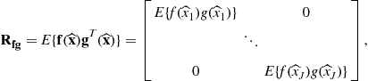 (21.117)
i.e., the covariances ![]() are all zero. It should be noted that for odd
are all zero. It should be noted that for odd ![]() and
and ![]() , if the probability density function of each zero-mean source signal is even, then the terms of the form
, if the probability density function of each zero-mean source signal is even, then the terms of the form ![]() equal zero. The true general condition for the statistical independence of signals is the vanishing of all high-order cross-cumulants [93–95]. The diagonalization principle can be expressed as
equal zero. The true general condition for the statistical independence of signals is the vanishing of all high-order cross-cumulants [93–95]. The diagonalization principle can be expressed as
![]() (21.118)
(21.118)
where ![]() is any diagonal positive definite matrix (typically,
is any diagonal positive definite matrix (typically, ![]() ). By pre-multiplying the above equation by the matrices
). By pre-multiplying the above equation by the matrices ![]() and
and ![]() , we obtain:
, we obtain:
![]() (21.119)
(21.119)
which suggests the following simple iterative multiplicative learning algorithm [96]
![]() (21.120)
(21.120)
![]() (21.121)
(21.121)
where the last equation represents the symmetric orthogonalization that keeps the algorithm stable. The above algorithm is very simple, but it needs the prewhitening of the sensor data and it is sensitive to noise [14,97].
Assuming prior knowledge of the source distributions ![]() , we can estimate
, we can estimate ![]() by using maximum likelihood (ML):
by using maximum likelihood (ML):
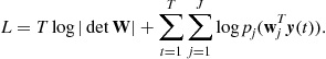 (21.122)
Using the gradient descent of the likelihood we obtain the infomax update rule
 (21.123)
where ![]() and
and ![]() is an entry-wise nonlinear score function defined by:
is an entry-wise nonlinear score function defined by:
![]() (21.124)
(21.124)
Using the natural gradient descent to increase the likelihood we get [98]:
 (21.125)
Alternatively, for signals corrupted by additive Gaussian noise, we can use higher order matrix cumulants. As an illustrative example, let us consider the following cost function which is a measure of independence [99]:
![]() (21.126)
(21.126)
where we use the following notations: ![]() denotes the q-order cumulants of the signal
denotes the q-order cumulants of the signal ![]() and
and ![]() denotes the cross-cumulant matrix whose elements are
denotes the cross-cumulant matrix whose elements are ![]() .
.
The first term in (21.126) assures that the determinant of the global matrix will not approach zero. By including this term we avoid the trivial solution ![]() . The second term forces the output signals to be as far as possible from Gaussianity, since the higher order cumulants are a natural measure of non-Gaussianity and they will vanish for Gaussian signals. It can be shown that for such a cost function, we can derive the following equivariant and robust (with respect to the Gaussian noise) algorithm [87,99,102]
. The second term forces the output signals to be as far as possible from Gaussianity, since the higher order cumulants are a natural measure of non-Gaussianity and they will vanish for Gaussian signals. It can be shown that for such a cost function, we can derive the following equivariant and robust (with respect to the Gaussian noise) algorithm [87,99,102]
![]() (21.127)
(21.127)
where ![]() and
and ![]() .
.
A wide class of equivariant algorithms for ICA can be expressed in a general form as (see Table 21.1) [14]
![]() (21.128)
(21.128)
where ![]() and the matrix
and the matrix ![]() can take different forms, for example
can take different forms, for example ![]() with suitably chosen nonlinearities
with suitably chosen nonlinearities ![]() and
and ![]() [14,95,96,99].
[14,95,96,99].
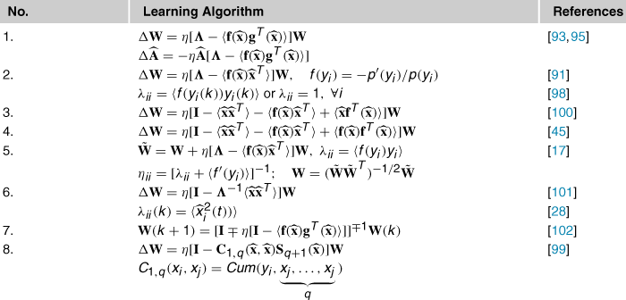
It should be noted that ICA based on HOS can perform blind source separation, i.e., allows us to estimate the true sources only if they are all statistically independent and are non Gaussian (except possibly of one) [14,91].
1.21.3.4 Blind source extraction
There are two main approaches to solve the problem of blind source separation. The first approach, which was mentioned briefly in the previous section, is to simultaneously separate all sources. In the second approach, we extract the sources sequentially in a blind fashion, one by one, rather than separating them all simultaneously. In many applications a large number of sensors (electrodes, sensors, microphones or transducers) are available but only a very few source signals are the subject of interest. For example, in the modern EEG or MEG devices, we typically observe more than 100 sensor signals, but only a few source signals are interesting; the rest can be considered as interfering noise. In another example, the cocktail party problem, it is usually essential to extract the voices of specific persons rather than separate all the source signals of all speakers available (in mixing form) from an array of microphones. For such applications it is essential to apply reliable, robust and effective learning algorithms which enable us to extract only a small number of source signals that are potentially interesting and contain useful information.
The blind source extraction (BSE) approach has several advantages over the simultaneous blind separation/deconvolution, such as