
Random Signals and Stochastic Processes
Luiz Wagner Pereira Biscainho, DEL/Poli & PEE/COPPE, Universidade Federal do Rio de Janeiro, Rio de Janeiro, Brazil
Abstract
This chapter is divided in three main parts. First, the main concepts of Probability are introduced. In the sequence, they are encapsulated into the Random Variable framework; a brief discussion of estimators is provided as an application example. At last, Random Processes and Sequences are tackled. After their detailed presentation, noise models, and modulation, spectral characterization and sampling of random processes are briefly discussed. The description of linear time-invariant processing of stationary processes and sequences leads to applications like Wiener filtering and special models for random signals.
Keywords
Probability; Random variable; Random process; Random sequence; Linear time-invariant system
Acknowledgements
The author thanks Dr. Paulo A.A. Esquef for carefully reviewing this manuscript and Leonardo de O. Nunes for kindly preparing the illustrations.
1.04.1 Introduction
Probability is an abstract concept useful to model chance experiments. The definition of a numerical representation for the outcomes of such experiments (the random variable) is essential to build a complete and general framework for probabilistic models. Such models can be extended to non-static outcomes in the form of time signals,1 leading to the so-called stochastic process, which can evolve along continuous or discrete time. Its complete description is usually too complicated to be applied to practical situations. Fortunately, a well-accepted set of simplifying properties like stationarity and ergodicity allows the modeling of many problems in so different areas as Biology, Economics, and Communications.
There are plenty of books on random processes,2 each one following some preferred order and notation, but covering essentially the same topics. This chapter is just one more attempt to present the subject in a compact manner. It is structured in the usual way: probability is first introduced, then described through random variables; within this framework, stochastic processes are presented, then associated with processing systems. Due to space limitations, proofs were avoided, and examples were kept at a minimum. No attempt was made to cover many families of probability distributions, for example. The preferred path was to define clear and unambiguously the concepts and entities associated to the subject and whenever possible give them simple and intuitive interpretations. Even risking to seem redundant, the author decided to explicitly duplicate the formulations related to random processes and sequences (i.e., continuous- and discrete-time random processes); the idea was to provide always a direct response to a consulting reader, instead of suggesting modifications in the given expressions.
Writing technical material always poses a difficult problem: which level of detail and depth will make the text useful? Our goal was making the text approachable for an undergraduate student as well as a consistent reference for more advanced students or even researchers (re)visiting random processes. The author tried to be especially careful with the notation consistence throughout the chapter in order to avoid confusion and ambiguity (which may easily occur in advanced texts). The choices of covered topics and order of presentation reflect several years of teaching the subject, and obviously match those of some preferred books. A selected list of didactic references on statistics [1,2], random variables and processes [3,4], and applications [5,6] is given at the end of the chapter. We hope you enjoy the reading.
1.04.2 Probability
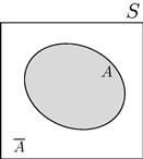
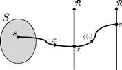
Probabilistic models are useful to describe and study phenomena that cannot be precisely predicted. To establish a precise framework for the concept of probability, one should define a chance experiment, of which each trial yields an outcome s. The set of all possible outcomes is the sample space S. In this context, one speaks of the probability that one trial of the experiment yields an outcome s that belongs to a desired set ![]() (when one says the event A has occurred), as illustrated in Figure 4.1.
(when one says the event A has occurred), as illustrated in Figure 4.1.

There are two different views of probability: the subjectivist and the objectivist. For subjectivists, the probability measures someone’s degree of belief on the occurrence of a given event, while for objectivists it results from concrete reality. Polemics aside, objectivism can be more rewarding didactically.
From the objectivist view point, one of the possible ways to define probability is the so-called classical or a priori approach: given an experiment whose possible outcomes s are equally likely, the probability of an event A is defined as the ratio between the number ![]() of acceptable outcomes (elements of A) and the number
of acceptable outcomes (elements of A) and the number ![]() of possible outcomes (elements of S):
of possible outcomes (elements of S):
![]() (4.1)
(4.1)
The experiment of flipping a fair coin, with ![]() , is an example in which the probabilities of both individual outcomes can be theoretically set:
, is an example in which the probabilities of both individual outcomes can be theoretically set: ![]() .
.
Another way to define probability is the relative frequency or a posteriori approach: the probability that the event A occurs after one trial of a given experiment can be obtained by taking the limit of the ratio between the number ![]() of successes (i.e., occurrences of A) and the number n of experiment trials, when the repeats go to infinity:
of successes (i.e., occurrences of A) and the number n of experiment trials, when the repeats go to infinity:
![]() (4.2)
(4.2)
In the ideal coin flip experiment, one is expected to find equal probabilities for head and tail. On the other hand, this pragmatic approach allows modeling the non-ideal case, provided the experiment can be repeated.
A pure mathematical definition can provide a sufficiently general framework to encompass every conceptual choice: the axiomatic approach develops a complete probability theory from three axioms:
Referring to an experiment with sample space S:
• The events ![]() , are said to be mutually exclusive when the occurrence of one prevents the occurrence of the others. They are the subject of the third axiom.
, are said to be mutually exclusive when the occurrence of one prevents the occurrence of the others. They are the subject of the third axiom.
• The complement![]() of a given event A, illustrated in Figure 4.2, is determined by the non-occurrence of A, i.e.,
of a given event A, illustrated in Figure 4.2, is determined by the non-occurrence of A, i.e., ![]() . From this definition,
. From this definition, ![]() . Complementary events are also mutually exclusive.
. Complementary events are also mutually exclusive.
It should be emphasized that all events A related to a given experiment are completely determined by the sample space S, since by definition ![]() . Therefore, a set B of outcomes not in S is mapped to an event
. Therefore, a set B of outcomes not in S is mapped to an event ![]() . For instance, for the experiment of rolling a fair die,
. For instance, for the experiment of rolling a fair die, ![]() ; the event corresponding to
; the event corresponding to ![]() (showing a 7) is
(showing a 7) is ![]() .
.
According to the experiment, sample spaces may be countable or uncountable.3 For example, the sample space of the coin flip experiment is countable. On the other hand, the sample space of the experiment that consists in sampling with no preference any real number from the interval ![]() is uncountable. Given an individual outcome
is uncountable. Given an individual outcome ![]() , defining
, defining ![]() ,
,
 (4.3)
(4.3)
As a consequence, one should not be surprised to find an event ![]() with
with ![]() or an event
or an event ![]() with
with ![]() . In the
. In the ![]() interval sampling experiment,
interval sampling experiment, ![]() has
has ![]() ; and
; and ![]() has
has ![]() .
.
1.04.2.1 Joint, conditional, and total probability—Bayes’ rule
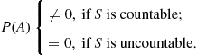
The joint probability of a set of events ![]() , is the probability of their simultaneous occurrence
, is the probability of their simultaneous occurrence ![]() . Referring to Figure 4.3, given two events A and B, their joint probability can be found as
. Referring to Figure 4.3, given two events A and B, their joint probability can be found as
![]() (4.4)
(4.4)
By rewriting this equation as
![]() (4.5)
(4.5)
one finds an intuitive result: the term ![]() is included twice in
is included twice in ![]() , and should thus be discounted. Moreover, when A and B are mutually exclusive, we arrive at the third axiom. In the die experiment, defining
, and should thus be discounted. Moreover, when A and B are mutually exclusive, we arrive at the third axiom. In the die experiment, defining ![]() and
and ![]() , and
, and ![]() .
.
The conditional probability![]() is the probability of event A conditioned to the occurrence of event B, and can be computed as
is the probability of event A conditioned to the occurrence of event B, and can be computed as
![]() (4.6)
(4.6)
The value of ![]() accounts for the uncertainty of both A and B; the term
accounts for the uncertainty of both A and B; the term ![]() discounts the uncertainty of B, since it is certain in this context. In fact, the conditioning event B is the new (reduced) sample space for the experiment. By rewriting this equation as
discounts the uncertainty of B, since it is certain in this context. In fact, the conditioning event B is the new (reduced) sample space for the experiment. By rewriting this equation as
![]() (4.7)
(4.7)
one gets another interpretation: the joint probability of A and B combines the uncertainty of B with the uncertainty of A when B is known to occur. Using the example in the last paragraph, ![]() in sample space
in sample space ![]() .
.
Since ![]() , the Bayes Rule follows straightforwardly:
, the Bayes Rule follows straightforwardly:
![]() (4.8)
(4.8)
This formula allows computing one conditional probability ![]() from its reverse
from its reverse ![]() . Using again the example in the last paragraph, one would arrive at the same result for
. Using again the example in the last paragraph, one would arrive at the same result for ![]() using
using ![]() in sample space
in sample space ![]() in the last equation.
in the last equation.
If the sample space S is partitioned into M disjoint sets ![]() , such that
, such that ![]() , then any event
, then any event ![]() can be written as
can be written as ![]() . Since
. Since ![]() , are disjoint sets,
, are disjoint sets,
 (4.9)
(4.9)
which is called the total probability of B.
For a single event of interest A, for example, the application of Eq. (4.9) to Eq. (4.8) yields
![]() (4.10)
(4.10)
Within the Bayes context, ![]() and
and ![]() are usually known as the a priori and a posteriori probabilities of A, respectively;
are usually known as the a priori and a posteriori probabilities of A, respectively; ![]() is called likelihood in the estimation context, and also transition probability in the communications context. In the latter case,
is called likelihood in the estimation context, and also transition probability in the communications context. In the latter case, ![]() could refer to a symbol a sent by the transmitter and
could refer to a symbol a sent by the transmitter and ![]() , to a symbol b recognized by the receiver. Knowing
, to a symbol b recognized by the receiver. Knowing ![]() , the probability of recognizing b when a is sent (which models the communication channel), and
, the probability of recognizing b when a is sent (which models the communication channel), and ![]() , the a priori probability of the transmitter to send a, allows to compute
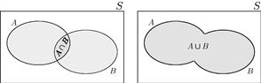
, the a priori probability of the transmitter to send a, allows to compute ![]() , the probability of a having been sent given that b has been recognized. In the case of binary communication, we could partition the sample space either in the events TX0 (0 transmitted) and TX1 (1 transmitted), or in the events RX0 (0 recognized) and RX1 (1 recognized), as illustrated in Figure 4.4; the event “error” would be
, the probability of a having been sent given that b has been recognized. In the case of binary communication, we could partition the sample space either in the events TX0 (0 transmitted) and TX1 (1 transmitted), or in the events RX0 (0 recognized) and RX1 (1 recognized), as illustrated in Figure 4.4; the event “error” would be ![]() .
.
1.04.2.2 Probabilistic independence
The events ![]() are said to be mutually independent when the occurrence of one does not affect the occurrence of any combination of the others.
are said to be mutually independent when the occurrence of one does not affect the occurrence of any combination of the others.
For two events A and B, three equivalent tests can be employed: they are independent if and only if.
The first two conditions follow directly from the definition of independence. Using any of them in Eq. (4.6) one arrives at the third one. The reader is invited to return to Eq. (4.7) and conclude that B and ![]() are independent events. Consider the experiment of rolling a special die with the numbers 1, 2, and 3 stamped in black on three faces and stamped in red on the other three; the events
are independent events. Consider the experiment of rolling a special die with the numbers 1, 2, and 3 stamped in black on three faces and stamped in red on the other three; the events ![]() and
and ![]() are mutually independent.
are mutually independent.
Algorithmically, the best choice for testing the mutual independence of more than two events is using the third condition for every combination of ![]() events among
events among ![]() .
.
As a final observation, mutually exclusive events are not mutually independent; on the contrary, one could say they are maximally dependent, since the occurrence of one precludes the occurrence of the other.
1.04.2.3 Combined experiments—Bernoulli trials
The theory we have discussed so far can be applied when more than one experiment is performed at a time. The generalization to the multiple experiment case can be easily done by using cartesian products.
Consider the experiments ![]() with their respective sample spaces
with their respective sample spaces ![]() . Define the combined experiment E such that each of its trials is composed by one trial of each
. Define the combined experiment E such that each of its trials is composed by one trial of each ![]() . An outcome of E is the M-tuple
. An outcome of E is the M-tuple ![]() , where
, where ![]() , and the sample space of E can be written as
, and the sample space of E can be written as ![]() . Analogously, any event of E can be expressed as
. Analogously, any event of E can be expressed as ![]() , where
, where ![]() is a properly chosen event of
is a properly chosen event of ![]() .
.
In the special case when the sub-experiments are mutually independent, i.e., the outcomes of one do not affect the outcomes of the others, we have ![]() . However, this is not the general case. Consider the experiment of randomly selecting a card from a 52-card deck, repeated twice: if the first card drawn is replaced, the sub-experiments are independent; if not, the first outcome affects the second experiment. For example, for
. However, this is not the general case. Consider the experiment of randomly selecting a card from a 52-card deck, repeated twice: if the first card drawn is replaced, the sub-experiments are independent; if not, the first outcome affects the second experiment. For example, for ![]() if the first card is replaced, and
if the first card is replaced, and ![]() if not.
if not.
At this point, an interesting counting experiment (called Bernoulli trials) can be defined. Take a random experiment E with sample space S and a desired event A (success) with ![]() , which also defines
, which also defines ![]() (failure) with
(failure) with ![]() . What is the probability of getting exactly k successes in N independent repeats of E? The solution can be easily found by noticing that the desired result is composed by k successes and
. What is the probability of getting exactly k successes in N independent repeats of E? The solution can be easily found by noticing that the desired result is composed by k successes and ![]() failures, which may occur in
failures, which may occur in ![]() different orders. Then,
different orders. Then,
 (4.11)
![]() (4.12)
(4.12)
Returning to the card deck experiment (with replacement): the probability of selecting exactly 2 aces of spades after 300 repeats is approximately 5.09% according to Eq. (4.11), while Eq. (4.12) provides the approximate value 5.20%. In a binary communication system where 0 and 1 are randomly transmitted with equal probabilities, the probability that exactly 2 bits 1 are sent among 3 bits transmitted is 0.25%; this result can be easily checked by inspection of Figure 4.5.

1.04.3 Random variable
Mapping each outcome of a random experiment to a real number provides a different framework for the study of probabilistic models, amenable to simple interpretation and easy mathematical manipulation. This mapping is performed by the so-called random variable.
Given a random experiment with sample space S, a random variable is any function ![]() that maps each
that maps each ![]() into some
into some ![]() (see Figure 4.6). The image of this transformation with domain S and co-domain
(see Figure 4.6). The image of this transformation with domain S and co-domain ![]() , which results of the convenient choice of the mapping function, can be seen as the sample space of
, which results of the convenient choice of the mapping function, can be seen as the sample space of ![]() ; any event A of
; any event A of ![]() can be described as a subset of
can be described as a subset of ![]() ; and each mapped outcome x is called a sample of
; and each mapped outcome x is called a sample of ![]() . The following conditions should be satisfied by a random variable
. The following conditions should be satisfied by a random variable ![]() :
:
We will see later that these conditions allow the proper definition of the cumulative probability distribution function of ![]() .
.

As seen in Section 1.04.2, sample spaces (and events) can be countable or uncountable, according to the nature of the random experiment’s individual outcomes. After mapped into subsets of ![]() , countable events remain countable—e.g., one could associate with the coin flip experiment a random variable
, countable events remain countable—e.g., one could associate with the coin flip experiment a random variable ![]() such that
such that ![]() and
and ![]() . On the other hand, uncountable events may or may not remain uncountable. Consider the following four distinct definitions of a random variable
. On the other hand, uncountable events may or may not remain uncountable. Consider the following four distinct definitions of a random variable ![]() associated with the
associated with the ![]() interval experiment described immediately before Eq. (4.3):
interval experiment described immediately before Eq. (4.3):


The sample space of:
The classification of sample spaces as countable or uncountable leads directly to the classification of random variables as discrete, continuous, or mixed. A discrete random variable ![]() has a countable sample space
has a countable sample space ![]() , and has
, and has ![]() —this is the case of
—this is the case of ![]() and
and ![]() defined above. A continuous random variable
defined above. A continuous random variable ![]() has an uncountable sample space
has an uncountable sample space ![]() , and (to avoid ambiguity) has
, and (to avoid ambiguity) has ![]() —this is the case of
—this is the case of ![]() defined above. A mixed variable
defined above. A mixed variable ![]() has a sample space
has a sample space ![]() composed by the union of real intervals with continuously distributed probabilities, within which
composed by the union of real intervals with continuously distributed probabilities, within which ![]() , and discrete real values with finite probabilities
, and discrete real values with finite probabilities ![]() —this is the case of
—this is the case of ![]() and
and ![]() defined above. Specifically, since
defined above. Specifically, since ![]() ,
, ![]() should rather be treated as part uncountable, part countable than as simply uncountable.
should rather be treated as part uncountable, part countable than as simply uncountable.
1.04.3.1 Probability distributions
From the conditions that must be satisfied by any random variable ![]() , an overall description of its probability distribution can be provided by the so-called cumulative probability distribution function (shortened to CDF),
, an overall description of its probability distribution can be provided by the so-called cumulative probability distribution function (shortened to CDF),
![]() (4.13)
(4.13)
Since ![]() . It is obvious that
. It is obvious that ![]() ; but since
; but since ![]() . Moreover,
. Moreover, ![]() and is a non-decreasing function of x, i.e.,
and is a non-decreasing function of x, i.e., ![]() . Also,
. Also, ![]() , i.e.,
, i.e., ![]() is continuous from the right; this will be important in the treatment of discrete random variables. A typical CDF is depicted in Figure 4.7. One can use the CDF to calculate probabilities by noticing that
is continuous from the right; this will be important in the treatment of discrete random variables. A typical CDF is depicted in Figure 4.7. One can use the CDF to calculate probabilities by noticing that
![]() (4.14)
(4.14)
For the random variable ![]() whose distribution is described in Figure 4.7, one can easily check by inspection that
whose distribution is described in Figure 4.7, one can easily check by inspection that ![]() .
.

The CDF of the random variable ![]() associated above with the
associated above with the ![]() interval sampling experiment is
interval sampling experiment is
 (4.15)
The CDF of the random variable ![]() associated above with the coin flip experiment is
associated above with the coin flip experiment is
 (4.16)
Given a random variable ![]() , any single value
, any single value ![]() such that
such that ![]() contributes a step4 of amplitude p to
contributes a step4 of amplitude p to ![]() . Then, it is easy to conclude that for a discrete random variable
. Then, it is easy to conclude that for a discrete random variable ![]() with
with ![]() ,
,
![]() (4.17)
(4.17)
An even more informative function that can be derived from the CDF to describe the probability distribution of a random variable ![]() is the so-called probability density function (shortened to PDF),
is the so-called probability density function (shortened to PDF),
![]() (4.18)
(4.18)
Since ![]() is a non-decreasing function of x, it follows that
is a non-decreasing function of x, it follows that ![]() . From the definition,
. From the definition,
![]() (4.19)
(4.19)
Then,
![]() (4.20)
(4.20)
The PDF corresponding to the CDF shown in Figure 4.7 is depicted in Figure 4.8. One can use the PDF to calculate probabilities by noticing that
![]() (4.21)
(4.21)
Again, for the random variable ![]() whose distribution is described in Figure 4.8, one can easily check by inspection that
whose distribution is described in Figure 4.8, one can easily check by inspection that ![]() .
.
The PDF of the random variable ![]() associated above with the
associated above with the ![]() interval sampling experiment is
interval sampling experiment is
 (4.22)
The PDF of the random variable ![]() associated above with the coin flip experiment is
associated above with the coin flip experiment is
 (4.23)
which is not well-defined. But coherently with what has been seen for the CDF, given a random variable ![]() , any single value
, any single value ![]() such that
such that ![]() contributes an impulse5 of area p to
contributes an impulse5 of area p to ![]() . Then, it is easy to conclude that for a discrete random variable
. Then, it is easy to conclude that for a discrete random variable ![]() with
with ![]() ,
,
![]() (4.24)
(4.24)
In particular, for the coin flip experiment the PDF is ![]() .
.
In the case of discrete random variables, in order to avoid the impulses in the PDF, one can operate directly on the so-called mass probability function6:
![]() (4.25)
(4.25)
In this case,
![]() (4.26)
(4.26)
This chapter favors an integrate framework for continuous and discrete variables, based on CDFs and PDFs.
It is usual in the literature referring (for short) to the CDF as “the distribution” and to the PDF as “the density” of the random variable. This text avoids this loose terminology, since the word “distribution” better applies to the overall probabilistic behavior of the random variable, no matter in the form of a CDF or a PDF.
1.04.3.2 Usual distributions
The simplest continuous distribution is the so-called uniform. A random variable ![]() is said to be uniformly distributed between a and
is said to be uniformly distributed between a and ![]() if its PDF is
if its PDF is
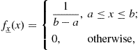 (4.27)
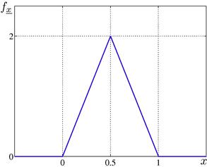
depicted in Figure 4.9. Notice that the inclusion or not of the interval bounds is unimportant here, since the variable is continuous. The error produced by uniform quantization of real numbers is an example of uniform random variable.

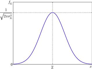
Perhaps the most recurrent continuous distribution is the so-called Gaussian (or normal). A Gaussian random variable ![]() is described by the PDF
is described by the PDF
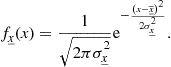 (4.28)
As seen in Figure 4.10, this function is symmetrical around ![]() , with spread controlled by
, with spread controlled by ![]() . These parameters, respectively called statistical mean and standard deviation of
. These parameters, respectively called statistical mean and standard deviation of ![]() , will be precisely defined in Section 1.04.3.4. The Gaussian distribution arises from the combination of several independent random phenomena, and is often associated with noise models.
, will be precisely defined in Section 1.04.3.4. The Gaussian distribution arises from the combination of several independent random phenomena, and is often associated with noise models.
There is no closed expression for the Gaussian CDF, which is usually tabulated for a normalized Gaussian random variable ![]() with
with ![]() and
and ![]() such that
such that
![]() (4.29)
(4.29)
In order to compute ![]() for a Gaussian random variable
for a Gaussian random variable ![]() , one can build an auxiliary variable
, one can build an auxiliary variable ![]() such that
such that ![]() , which can then be approximated by tabulated values of
, which can then be approximated by tabulated values of ![]() .
.
Example 1
The values r of a 10-% resistor series produced by a component industry can be modeled by a Gaussian random variable ![]() with
with ![]() . What is the probability of producing a resistor within
. What is the probability of producing a resistor within ![]() of
of ![]() ?
?
Solution 1
The normalized counterpart of ![]() is
is ![]() . Then,
. Then,
![]() (4.30)
(4.30)
Notice once more that since the variable is continuous, the inclusion or not of the interval bounds has no influence on the result.
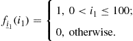
In Section 1.04.2.3, an important discrete random variable was implicitly defined. A random variable ![]() that follows the so-called binomial distribution is described by
that follows the so-called binomial distribution is described by
 (4.31)
and counts the number of occurrences of an event A which has probability p, after N independent repeats of a random experiment. Games of chance are related to binomial random variables.
The so-called Poisson distribution, described by
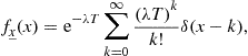 (4.32)
counts the number of occurrences of an event A that follows a mean rate of ![]() occurrences per unit time, during the time interval T. Traffic studies are related to Poisson random variables.
occurrences per unit time, during the time interval T. Traffic studies are related to Poisson random variables.
It is simple to derive the Poisson distribution from the binomial distribution. If an event A may occur with no preference anytime during a time interval ![]() , the probability that A occurs within the time interval
, the probability that A occurs within the time interval ![]() is
is ![]() . If A occurs N times in
. If A occurs N times in ![]() , the probability that it falls exactly k times in
, the probability that it falls exactly k times in ![]() is
is 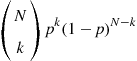 . If
. If ![]() ; if A follows a mean rate of
; if A follows a mean rate of ![]() occurrences per unit time, then
occurrences per unit time, then ![]() and the probability of exact k occurrences in a time interval of duration T becomes
and the probability of exact k occurrences in a time interval of duration T becomes ![]() , where
, where ![]() substituted for Np. If a central office receives 100 telephone calls per minute in the mean, the probability that more than 1 call arrive during 1s is
substituted for Np. If a central office receives 100 telephone calls per minute in the mean, the probability that more than 1 call arrive during 1s is ![]() .
.
Due to space restrictions, this chapter does not detail other random distributions, which can be easily found in the literature.
1.04.3.3 Conditional distribution
In many instances, one is interested in studying the behavior of a given random variable ![]() under some constraints. A conditional distribution can be built to this effect, if the event
under some constraints. A conditional distribution can be built to this effect, if the event ![]() summarizes those constraints. The corresponding CDF of
summarizes those constraints. The corresponding CDF of ![]() conditioned to B can be computed as
conditioned to B can be computed as
![]() (4.33)
(4.33)
The related PDF is simply
![]() (4.34)
(4.34)
Conditional probabilities can be straightforwardly computed from conditional CDFs or PDFs.
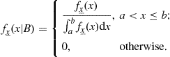
When the conditioning event is an interval ![]() , it can be easily deduced that
, it can be easily deduced that
 (4.35)
and
 (4.36)
Both sentences in Eq. (4.36) can be easily interpreted:
• Within ![]() , the conditional PDF has the same shape of the original one; the normalization factor
, the conditional PDF has the same shape of the original one; the normalization factor ![]() ensures
ensures ![]() in the restricted sample space
in the restricted sample space ![]() .
.
• By definition, there is null probability of getting x outside ![]() .
.
As an example, the random variable H defined by the non-negative outcomes of a normalized Gaussian variable follows the PDF
![]() (4.37)
(4.37)
The results shown in this section can be promptly generalized to any conditioning event.
1.04.3.4 Statistical moments
The concept of mean does not need any special introduction: the single value that substituted for each member in a set of numbers produces the same total. In the context of probability, following a frequentist path, one could define the arithmetic mean of infinite samples of a random variable ![]() as its statistical mean
as its statistical mean![]() or its expected value
or its expected value![]() .
.
Recall the random variable ![]() associated with the fair coin flip experiment, with
associated with the fair coin flip experiment, with ![]() . After infinite repeats of the experiment, one gets 50% of heads (
. After infinite repeats of the experiment, one gets 50% of heads (![]() ) and 50% of tails (
) and 50% of tails (![]() ); then, the mean outcome will be7
); then, the mean outcome will be7![]() . If another variable
. If another variable ![]() is associated with an unfair coin with probabilities
is associated with an unfair coin with probabilities ![]() and
and ![]() , the same reasoning leads to
, the same reasoning leads to ![]() . Instead of averaging infinite outcomes, just summing the possible values of the random variable weighted by their respective probabilities also yields its statistical mean. Thus we can state that for any discrete random variable
. Instead of averaging infinite outcomes, just summing the possible values of the random variable weighted by their respective probabilities also yields its statistical mean. Thus we can state that for any discrete random variable ![]() with sample space
with sample space ![]() ,
,
![]() (4.38)
(4.38)
This result can be generalized. Given a continuous random variable ![]() , the probability of drawing a value in the interval
, the probability of drawing a value in the interval ![]() around
around ![]() is given by
is given by ![]() . The weighted sum of every
. The weighted sum of every ![]() is simply
is simply
![]() (4.39)
(4.39)
By substituting the PDF of a discrete variable ![]() (see Eq. (4.24)) into this expression, one arrives at Eq. (4.38). Then, Eq. (4.39) is the analytic expression for the expected value of any random variable
(see Eq. (4.24)) into this expression, one arrives at Eq. (4.38). Then, Eq. (4.39) is the analytic expression for the expected value of any random variable ![]() .
.
Suppose another random variable ![]() is built as a function of
is built as a function of ![]() . Since the probability of getting the value
. Since the probability of getting the value ![]() is the same as getting the respective
is the same as getting the respective ![]() , we can deduce that
, we can deduce that
![]() (4.40)
(4.40)
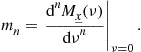
A complete family of measures based on expected values can be associated with a random variable. The so-called nth-order moment of ![]() (about the origin) is defined as
(about the origin) is defined as
![]() (4.41)
(4.41)
The first two moments of ![]() are:
are:
A modified family of parameters can be formed by computing the moments about the mean. The so-called nth-order central moment of ![]() is defined as
is defined as
![]() (4.42)
(4.42)
Subtracting the statistical mean from a random variable can be interpreted as disregarding its “deterministic” part (represented by its statistical mean) Three special cases:
• ![]() , known as the variance of
, known as the variance of ![]() , which measures the spread of
, which measures the spread of ![]() around
around ![]() . The so-called standard deviation
. The so-called standard deviation![]() is a convenient measure with the same dimension of
is a convenient measure with the same dimension of ![]() .
.
• ![]() , whose standardized version
, whose standardized version ![]() is the so-called skewness of
is the so-called skewness of ![]() , which measures the asymmetry of
, which measures the asymmetry of ![]() .
.
• ![]() , whose standardized version8 minus three
, whose standardized version8 minus three ![]() is the so-called kurtosis of
is the so-called kurtosis of ![]() , which measures the peakedness of
, which measures the peakedness of ![]() . One can say the distributions are measured against the Gaussian, which has a null kurtosis.
. One can say the distributions are measured against the Gaussian, which has a null kurtosis.
Of course, analogous definitions apply to the moments computed over conditional distributions.
A useful expression, which will be recalled in the context of random processes, relates three of the measures defined above:
![]() (4.43)
(4.43)
Rewritten as
![]() (4.44)
(4.44)
it allows to split the overall “intensity” of ![]() , measured by its mean square value, into a deterministic part, represented by
, measured by its mean square value, into a deterministic part, represented by ![]() , and a random part, represented by
, and a random part, represented by ![]() .
.
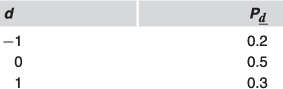
As an example, consider a discrete random variable ![]() distributed as shown in Table 4.1. Their respective parameters are:
distributed as shown in Table 4.1. Their respective parameters are:
• mean ![]() , indicating the PDF of
, indicating the PDF of ![]() is shifted to the right of the origin;
is shifted to the right of the origin;
• mean square value ![]() , which measures the intensity of
, which measures the intensity of ![]() ;
;
• variance ![]() , which measures the random part of the intensity of
, which measures the random part of the intensity of ![]() ;
;
• standard deviation ![]() , which measures the spread of
, which measures the spread of ![]() around its mean;
around its mean;
• skewness ![]() , indicating the PDF of
, indicating the PDF of ![]() is left-tailed;
is left-tailed;
• kurtosis ![]() , indicating the PDF of
, indicating the PDF of ![]() is less peaky than the PDF of a Gaussian variable.
is less peaky than the PDF of a Gaussian variable.
At this point, we can discuss two simple transformations of a random variable ![]() whose effects can be summarized by low-order moments:
whose effects can be summarized by low-order moments:
• A random variable ![]() can be formed by adding a fixed offset
can be formed by adding a fixed offset ![]() to each sample of
to each sample of ![]() . As a consequence of this operation, the new PDF is a shifted version of the original one:
. As a consequence of this operation, the new PDF is a shifted version of the original one: ![]() , thus adding
, thus adding ![]() to the mean of
to the mean of ![]() :
: ![]() .
.
• A random variable ![]() can be formed by scaling by
can be formed by scaling by ![]() each sample of
each sample of ![]() . As a consequence of this operation, the new PDF is a scaled version of the original one:
. As a consequence of this operation, the new PDF is a scaled version of the original one: ![]() , thus scaling by
, thus scaling by ![]() the standard deviation of
the standard deviation of ![]() :
: ![]() .
.
Such transformations do not change the shape (and therefore the type) of the original distribution. In particular, one can generate:
• a zero-mean version of ![]() by making
by making ![]() , which disregards the deterministic part of
, which disregards the deterministic part of ![]() ;
;
• a unit-standard deviation version of ![]() by making
by making ![]() , which enforces a standard statistical variability to
, which enforces a standard statistical variability to ![]() ;
;
• a normalized version of ![]() by making
by making ![]() , which combines both effects.
, which combines both effects.
We already defined a normalized Gaussian distribution in Section 1.04.3.2. The normalized version ![]() of the random variable
of the random variable ![]() of the last example would be distributed as shown in Table 4.2.
of the last example would be distributed as shown in Table 4.2.

The main importance of these expectation-based parameters is to provide a partial description of an underlying distribution without the need to resource to the PDF. In a practical situation in which only a few samples of a random variable are available, as opposed to its PDF and related moments, it is easier to get more reliable estimates for the latter (especially low-order ones) than for the PDF itself. The same rationale applies to the use of certain auxiliary inequalities that avoid the direct computation of probabilities on a random variable (which otherwise would require the knowledge or estimation of its PDF) by providing upper bounds for them based on low-order moments. Two such inequalities are:
The derivation of Markov’s inequality is quite simple:
 (4.45)
Chebyshev’s inequality follows directly by substituting ![]() for
for ![]() in Markov’s inequality. As an example, the probability of getting a sample
in Markov’s inequality. As an example, the probability of getting a sample ![]() from the normalized Gaussian random variable
from the normalized Gaussian random variable ![]() is
is ![]() ; Chebyshev’s inequality predicts
; Chebyshev’s inequality predicts ![]() , an upper bound almost 100 times greater than the actual probability.
, an upper bound almost 100 times greater than the actual probability.
Two representations of the distribution of a random variable in alternative domains provide interesting links with its statistical moments. The so-called characteristic function of a random variable ![]() is defined as
is defined as
![]() (4.46)
(4.46)
and inter-relates the moments ![]() by successive differentiations:
by successive differentiations:
 (4.47)
The so-called moment generating function of a random variable ![]() is defined as
is defined as
![]() (4.48)
(4.48)
and provides a more direct way to compute ![]() :
:
 (4.49)
1.04.3.5 Transformation of random variables
Consider the problem of describing a random variable ![]() obtained by transformation of another random variable
obtained by transformation of another random variable ![]() , illustrated in Figure 4.11. By definition,
, illustrated in Figure 4.11. By definition,
![]() (4.50)
(4.50)
If ![]() is a continuous random variable and
is a continuous random variable and ![]() is a differentiable function, the sentence
is a differentiable function, the sentence ![]() is equivalent to a set of sentences in the form
is equivalent to a set of sentences in the form ![]() . Since
. Since ![]() , then
, then ![]() can be expressed as a function of
can be expressed as a function of ![]() .
.
Fortunately, an intuitive formula expresses ![]() as a function of
as a function of ![]() :
:
 (4.51)
Given that the transformation ![]() is not necessarily monotonic,
is not necessarily monotonic, ![]() are all possible values mapped to y; therefore, their contributions must be summed up. It is reasonable that
are all possible values mapped to y; therefore, their contributions must be summed up. It is reasonable that ![]() must be directly proportional to
must be directly proportional to ![]() : the more frequent a given
: the more frequent a given ![]() , the more frequent its respective
, the more frequent its respective ![]() . By its turn, the term
. By its turn, the term ![]() accounts for the distortion imposed to
accounts for the distortion imposed to ![]() by
by ![]() . For example, if this transformation is almost constant in a given region, no matter if increasing or decreasing, then
. For example, if this transformation is almost constant in a given region, no matter if increasing or decreasing, then ![]() in the denominator will be close to zero; this just reflects the fact that a wide range of
in the denominator will be close to zero; this just reflects the fact that a wide range of ![]() values will be mapped into a narrow range of values of
values will be mapped into a narrow range of values of ![]() , which will then become denser than
, which will then become denser than ![]() in thar region.
in thar region.
As an example, consider that a continuous random variable ![]() is transformed into a new variable
is transformed into a new variable ![]() . For the CDF of
. For the CDF of ![]() ,
,
![]() (4.52)
(4.52)
By Eq. (4.51), or by differentiation of Eq. (4.52), one arrives at the PDF of ![]() :
:
![]() (4.53)
(4.53)
The case when real intervals of ![]() are mapped into single values of
are mapped into single values of ![]() requires an additional care to treat the nonzero individual probabilities of the resulting values of the new variable. However, the case of a discrete random variable
requires an additional care to treat the nonzero individual probabilities of the resulting values of the new variable. However, the case of a discrete random variable ![]() with
with ![]() being transformed is trivial:
being transformed is trivial:
![]() (4.54)
(4.54)
Again, ![]() are all possible values mapped to
are all possible values mapped to ![]() .
.
An interesting application of transformations of random variables is to obtain samples of a given random variable ![]() from samples of another random variable
from samples of another random variable ![]() , both with known distributions. Assume that exists
, both with known distributions. Assume that exists ![]() such that
such that ![]() . Then,
. Then, ![]() , which requires only the invertibility of
, which requires only the invertibility of ![]() .
.
1.04.3.6 Multiple random variable distributions
A single random experiment E (composed or not) may give rise to a set of N random variables, if each individual outcome ![]() is mapped into several real values
is mapped into several real values ![]() . Consider, for example, the random experiment of sampling the climate conditions at every point on the globe; daily mean temperature
. Consider, for example, the random experiment of sampling the climate conditions at every point on the globe; daily mean temperature ![]() and relative air humidity
and relative air humidity ![]() can be considered as two random variables that serve as numerical summarizing measures. One must generalize the probability distribution descriptions to cope with this multiple random variable situation: it should be clear that the set of N individual probability distribution descriptions, one for each distinct random variable, provides less information than their joint probability distribution description, since the former cannot convey information about their mutual influences.
can be considered as two random variables that serve as numerical summarizing measures. One must generalize the probability distribution descriptions to cope with this multiple random variable situation: it should be clear that the set of N individual probability distribution descriptions, one for each distinct random variable, provides less information than their joint probability distribution description, since the former cannot convey information about their mutual influences.
We start by defining a multiple or vector random variable as the function ![]() that maps
that maps ![]() into
into ![]() , such that
, such that
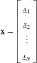 (4.55)
and
 (4.56)
Notice that ![]() are jointly sampled from
are jointly sampled from ![]() .
.
The joint cumulative probability distribution function of ![]() , or simply the CDF of
, or simply the CDF of ![]() , can be defined as
, can be defined as
![]() (4.57)
(4.57)
The following relevant properties of the joint CDF can be easily deduced:
Define ![]() containing
containing ![]() variables of interest among the random variables in
variables of interest among the random variables in ![]() , and leave the remaining
, and leave the remaining ![]() nuisance variables in
nuisance variables in ![]() . The so-called marginal CDF of
. The so-called marginal CDF of ![]() separately describes these variables’ distribution from the knowledge of the CDF of
separately describes these variables’ distribution from the knowledge of the CDF of ![]() :
:
![]() (4.58)
(4.58)
One says the variables ![]() have been marginalized out: the condition
have been marginalized out: the condition ![]() simply means they must be in the sample space, thus one does not need to care about them anymore.
simply means they must be in the sample space, thus one does not need to care about them anymore.
The CDF of a discrete random variable ![]() with
with ![]() , analogously to the single variable case, is composed by steps at the admissible N-tuples:
, analogously to the single variable case, is composed by steps at the admissible N-tuples:
![]() (4.59)
(4.59)
The joint probability density function of ![]() , or simply the PDF of
, or simply the PDF of ![]() , can be defined as
, can be defined as
![]() (4.60)
(4.60)
Since ![]() is a non-decreasing function of
is a non-decreasing function of ![]() , it follows that
, it follows that ![]() . From the definition,
. From the definition,
![]() (4.61)
(4.61)
![]() (4.62)
(4.62)
The probability of any event ![]() can be computed as
can be computed as
![]() (4.63)
(4.63)
Once more we can marginalize the nuisance variables ![]() to obtain the marginal PDF of
to obtain the marginal PDF of ![]() from the PDF of
from the PDF of ![]() :
:
![]() (4.64)
(4.64)
Notice that if ![]() and
and ![]() are statistically dependent, the marginalization of
are statistically dependent, the marginalization of ![]() does not “eliminate” the effect of
does not “eliminate” the effect of ![]() on
on ![]() : the integration is performed over
: the integration is performed over ![]() , which describes their mutual influences. For a discrete random variable
, which describes their mutual influences. For a discrete random variable ![]() with
with ![]() consists of impulses at the admissible N-tuples:
consists of impulses at the admissible N-tuples:
![]() (4.65)
(4.65)
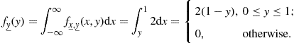
Suppose, for example, that we want to find the joint and marginal CDFs and PDFs of two random variables ![]() and
and ![]() jointly uniformly distributed in the region
jointly uniformly distributed in the region ![]() , i.e., such that
, i.e., such that
 (4.66)
The marginalization of ![]() yields
yields
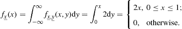 (4.67)
The marginalization of ![]() yields
yields
 (4.68)
By definition,
 (4.69)
The reader is invited to sketch the admissible region ![]() on the
on the ![]() plane and try to solve Eq. (4.69) by visual inspection. The marginal CDF of x is given by
plane and try to solve Eq. (4.69) by visual inspection. The marginal CDF of x is given by
 (4.70)
which could also have been obtained by direct integration of ![]() . The marginal CDF of y is given by
. The marginal CDF of y is given by
 (4.71)
which could also have been obtained by direct integration of ![]() .
.
Similarly to the univariate case discussed in Section 1.04.3.3, the conditional distribution of a vector random variable ![]() restricted by a conditioning event
restricted by a conditioning event ![]() can be described by its respective CDF
can be described by its respective CDF
![]() (4.72)
(4.72)
and PDF
![]() (4.73)
(4.73)
A special case arises when B imposes a point conditioning: Define ![]() containing
containing ![]() variables among those in
variables among those in ![]() , such that
, such that ![]() . It can be shown that
. It can be shown that
![]() (4.74)
(4.74)
an intuitive result in light of Eq. (4.6)—to which one may directly refer in the case of discrete random variables. Returning to the last example, the point-conditioned PDFs can be shown to be
 (4.75)
and
 (4.76)
1.04.3.7 Statistically independent random variables
Based on the concept of statistical independence, discussed in Section 1.04.2.2, the mutual statistical independence of a set of random variables means that the probabilistic behavior of each one is not affected by the probabilistic behavior of the others. Formally, the random variables ![]() are independent if any of the following conditions is fulfilled:
are independent if any of the following conditions is fulfilled:
Returning to the example developed in Section 1.04.3.6, x and y are clearly statistically dependent. However, if they were jointly uniformly distributed in the region defined by ![]() , they would be statistically independent—this verification is left to the reader.
, they would be statistically independent—this verification is left to the reader.
The PDF of a random variable ![]() composed by the sum of N independent variables
composed by the sum of N independent variables ![]() can be computed as9
can be computed as9
![]() (4.77)
(4.77)
1.04.3.8 Joint statistical moments
The definition of statistical mean can be directly extended to a vector random variable ![]() with known PDF. The expected value of a real scalar function
with known PDF. The expected value of a real scalar function ![]() is given by:
is given by:
![]() (4.78)
(4.78)
We can analogously proceed to the definition of N-variable joint statistical moments. However, due to the more specific usefulness of the ![]() cases, only 2-variable moments will be presented.
cases, only 2-variable moments will be presented.
An ![]() th-order joint moment of
th-order joint moment of ![]() and
and ![]() (about the origin) has the general form
(about the origin) has the general form
![]() (4.79)
(4.79)
The most important case corresponds to ![]() :
: ![]() is called the statistical correlation between
is called the statistical correlation between ![]() and
and ![]() . Under a frequentist perspective,
. Under a frequentist perspective, ![]() is the average of infinite products of samples x and y jointly drawn from
is the average of infinite products of samples x and y jointly drawn from ![]() , which links the correlation to an inner product between the random variables. Indeed, when
, which links the correlation to an inner product between the random variables. Indeed, when ![]() ,
, ![]() and
and ![]() are called orthogonal. One can say the correlation quantifies the overall linear relationship between the two variables. Moreover, when
are called orthogonal. One can say the correlation quantifies the overall linear relationship between the two variables. Moreover, when ![]() ,
, ![]() and
and ![]() are called mutually uncorrelated; this “separability” in the mean is weaker than the distribution separability implied by the independence. In fact, if
are called mutually uncorrelated; this “separability” in the mean is weaker than the distribution separability implied by the independence. In fact, if ![]() and
and ![]() are independent,
are independent,
 (4.80)
i.e., they are also uncorrelated. The converse is not necessarily true.
An ![]() th-order joint central moment of
th-order joint central moment of ![]() and
and ![]() , computed about the mean, has the general form
, computed about the mean, has the general form
![]() (4.81)
(4.81)
Once more, the case ![]() is specially important:
is specially important: ![]() is called the statistical covariance between
is called the statistical covariance between ![]() and
and ![]() , which quantifies the linear relationship between their random parts. Since10
, which quantifies the linear relationship between their random parts. Since10![]() ,
, ![]() and
and ![]() are uncorrelated when
are uncorrelated when ![]() . If
. If ![]() , one says
, one says ![]() and
and ![]() are positively correlated, i.e., the variations of their statistical samples tend to occur in the same direction; if
are positively correlated, i.e., the variations of their statistical samples tend to occur in the same direction; if ![]() , one says
, one says ![]() and
and ![]() are negatively correlated, i.e., the variations of their statistical samples tend to occur in opposite directions. For example, the age and the annual medical expenses of an individual are expected to be positively correlated random variables. A normalized covariance can be computed as the correlation between the normalized versions of
are negatively correlated, i.e., the variations of their statistical samples tend to occur in opposite directions. For example, the age and the annual medical expenses of an individual are expected to be positively correlated random variables. A normalized covariance can be computed as the correlation between the normalized versions of ![]() and
and ![]() :
:
 (4.82)
known as the correlation coefficient between ![]() and
and ![]() ,
, ![]() , and can be interpreted as the percentage of correlation between x and y. Recalling the inner product interpretation, the correlation coefficient can be seen as the cosine of the angle between the statistical variations of the two random variables.
, and can be interpreted as the percentage of correlation between x and y. Recalling the inner product interpretation, the correlation coefficient can be seen as the cosine of the angle between the statistical variations of the two random variables.
Consider, for example, the discrete variables ![]() and
and ![]() jointly distributed as shown in Table 4.3. Their joint second-order parameters are:
jointly distributed as shown in Table 4.3. Their joint second-order parameters are:
• correlation ![]() , indicating
, indicating ![]() and
and ![]() are not orthogonal;
are not orthogonal;
• covariance ![]() , indicating
, indicating ![]() and
and ![]() tend to evolve in opposite directions;
tend to evolve in opposite directions;
• correlation coefficient ![]() , indicating this negative correlation is relatively strong.
, indicating this negative correlation is relatively strong.

Returning to N-dimensional random variables, the characteristic function of a vector random variable ![]() is defined as
is defined as
![]() (4.83)
(4.83)
and inter-relates the moments of order ![]() by:
by:
 (4.84)
The moment generating function of a vector random variable ![]() is defined as
is defined as
![]() (4.85)
(4.85)
and allows the computation of ![]() as:
as:
 (4.86)
1.04.3.9 Central limit theorem
A result that partially justifies the ubiquitous use of Gaussian models, the Central Limit Theorem (CLT) states that (under mild conditions in practice) the distribution of a sum ![]() of N independent variables
of N independent variables ![]() approaches a Gaussian distribution as
approaches a Gaussian distribution as ![]() . Having completely avoided the CLT proof, we can at least recall that in this case,
. Having completely avoided the CLT proof, we can at least recall that in this case, ![]() (see Eq. (4.77). Of course,
(see Eq. (4.77). Of course, ![]() and, by the independence property,
and, by the independence property, ![]() .
.
Gaussian approximations for finite-N models are useful for sufficiently high N, but due to the shape of the Gaussian distribution, the approximation error grows as y distances from ![]() .
.
The reader is invited to verify the validity of the approximation provided by the CLT for successive sums of independent ![]() uniformly distributed in
uniformly distributed in ![]() .
.
Interestingly, the CLT also applies to the sum of discrete distributions: even if ![]() remains impulsive, the shape of
remains impulsive, the shape of ![]() approaches the shape of the CDF of a Gaussian random variable as N grows.
approaches the shape of the CDF of a Gaussian random variable as N grows.
1.04.3.10 Multivariate Gaussian distribution
The PDF of an N-dimensional Gaussian variable is defined as
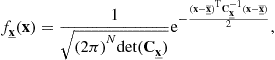 (4.87)
where ![]() is an
is an ![]() vector with elements
vector with elements ![]() , and
, and ![]() is an
is an ![]() matrix with elements
matrix with elements ![]() , such that any related marginal distribution remains Gaussian. As a consequence, by Eq. (4.74), any conditional distribution
, such that any related marginal distribution remains Gaussian. As a consequence, by Eq. (4.74), any conditional distribution ![]() with point conditioning B is also Gaussian.
with point conditioning B is also Gaussian.
By this definition, we can see the Gaussian distribution is completely defined by its first- and second-order moments, which means that if N jointly distributed random variables are known to be Gaussian, estimating their mean-vector![]() and their covariance-matrix
and their covariance-matrix![]() is equivalent to estimate their overall PDF. Moreover, if
is equivalent to estimate their overall PDF. Moreover, if ![]() and
and ![]() are mutually uncorrelated,
are mutually uncorrelated, ![]() , then
, then ![]() is diagonal, and the joint PDF becomes
is diagonal, and the joint PDF becomes ![]() , i.e.,
, i.e., ![]() will be mutually independent. This is a strong result inherent to Gaussian distributions.
will be mutually independent. This is a strong result inherent to Gaussian distributions.
1.04.3.11 Transformation of vector random variables
The treatment of a general multiple random variable ![]() resulting from the application of the transformation
resulting from the application of the transformation ![]() to the multiple variable
to the multiple variable ![]() always starts by enforcing
always starts by enforcing ![]() , with
, with ![]() .
.
The special case when ![]() is invertible, i.e.,
is invertible, i.e., ![]() (or
(or ![]() ), follows a closed expression:
), follows a closed expression:
![]() (4.88)
(4.88)
where
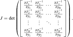 (4.89)
The reader should notice that this expression with ![]() reduces to Eq. (4.51) particularized to the invertible case.
reduces to Eq. (4.51) particularized to the invertible case.
Given the multiple random variable ![]() with known mean-vector
with known mean-vector ![]() and covariance-matrix
and covariance-matrix ![]() , its linear transformation
, its linear transformation ![]() will have:
will have:
It is possible to show that the linear transformation ![]() of an N-dimensional Gaussian random variable
of an N-dimensional Gaussian random variable ![]() is also Gaussian. Therefore, in this case the two expressions above completely determine the PDF of the transformed variable.
is also Gaussian. Therefore, in this case the two expressions above completely determine the PDF of the transformed variable.
The generation of samples that follow a desired multivariate probabilistic distribution from samples that follow another known multivariate probabilistic distribution applies the same reasoning followed in the univariate case to the multivariate framework. The reader is invited to show that given the pair ![]() of samples from the random variables
of samples from the random variables ![]() , jointly uniform in the region
, jointly uniform in the region ![]() , it is possible to generate the pair
, it is possible to generate the pair ![]() of samples from the random variables
of samples from the random variables ![]() , jointly Gaussian with the desired parameters
, jointly Gaussian with the desired parameters ![]() by making
by making
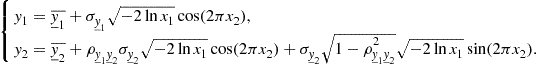 (4.90)
1.04.3.12 Complex random variables
At first sight, defining a complex random variable ![]() may seem impossible, since the seminal event
may seem impossible, since the seminal event ![]() makes no sense. However, in the vector random variable framework this issue can be circumvented if one jointly describes the real and imaginary parts (or magnitude and phase) of
makes no sense. However, in the vector random variable framework this issue can be circumvented if one jointly describes the real and imaginary parts (or magnitude and phase) of ![]() .
.
The single complex random variable ![]() , is completely represented by
, is completely represented by ![]() , which allows one to compute the expected value of a scalar function
, which allows one to compute the expected value of a scalar function ![]() as
as ![]() . Moreover, we can devise general definitions for the mean and variance of
. Moreover, we can devise general definitions for the mean and variance of ![]() as, respectively:
as, respectively:
An N-dimensional complex random variable ![]() can be easily tackled through a properly defined joint distribution, e.g.,
can be easily tackled through a properly defined joint distribution, e.g., ![]() . The individual variables
. The individual variables ![]() ,
, ![]() , will be independent when
, will be independent when
 (4.91)
The following definitions must be generalized to cope with complex random variables:
Now, ![]() . As before,
. As before, ![]() and
and ![]() will be:
will be:
1.04.3.13 An application: estimators
One of the most encompassing applications of vector random variables is the so-called parameter estimation, per se an area supported by its own theory. The typical framework comprises using a finite set of measured data from a given phenomenon to estimate the parameters11 of its underlying model.
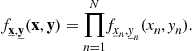
A set ![]() of N independent identically distributed (iid) random variables such that
of N independent identically distributed (iid) random variables such that
 (4.92)
can describe an N-size random sample of a population modeled by ![]() . Any function
. Any function ![]() (called a statistic of
(called a statistic of ![]() ) can constitute a point estimator
) can constitute a point estimator![]() of some parameter
of some parameter ![]() such that given an N-size sample
such that given an N-size sample ![]() of
of ![]() , one can compute an estimate
, one can compute an estimate ![]() of
of ![]() .
.
A classical example of point estimator for a fixed parameter is the so-called sample mean, which estimates ![]() by the arithmetic mean of the available samples
by the arithmetic mean of the available samples ![]() :
:
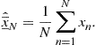 (4.93)
Not always defining a desired estimator is trivial task as in the previous example. In general, resorting to a proper analytical criterion is necessary. Suppose we are given the so-called likelihood function of ![]() ,
, ![]() , which provides a probabilistic model for
, which provides a probabilistic model for ![]() as an explicit function of
as an explicit function of ![]() . Given the sample
. Given the sample ![]() , the so-called maximum likelihood (ML) estimator
, the so-called maximum likelihood (ML) estimator ![]() computes an estimate of
computes an estimate of ![]() by direct maximization of
by direct maximization of ![]() . This operation is meant to find the value of
. This operation is meant to find the value of ![]() that would make the available sample
that would make the available sample ![]() most probable.
most probable.
Sometimes the parameter ![]() itself can be a sample of a random variable
itself can be a sample of a random variable ![]() described by an a priori PDF
described by an a priori PDF ![]() . For example, suppose one wants to estimate the mean value of a shipment of components received from a given factory; since the components may come from several production units, we can think of a statistical model for their nominal values. In such situations, any reliable information on the parameter distribution can be taken in account to better tune the estimator formulation; these so-called Bayesian estimators rely on the a posteriori PDF of
. For example, suppose one wants to estimate the mean value of a shipment of components received from a given factory; since the components may come from several production units, we can think of a statistical model for their nominal values. In such situations, any reliable information on the parameter distribution can be taken in account to better tune the estimator formulation; these so-called Bayesian estimators rely on the a posteriori PDF of ![]() :
:
![]() (4.94)
(4.94)
Given a sample ![]() , the so-called maximum a posteriori (MAP) estimator
, the so-called maximum a posteriori (MAP) estimator ![]() computes an estimate of
computes an estimate of ![]() as the mode of
as the mode of ![]() . This choice is meant to find the most probable
. This choice is meant to find the most probable ![]() that would have produced the available data
that would have produced the available data ![]() . Several applications favor the posterior mean estimator, which for a given sample
. Several applications favor the posterior mean estimator, which for a given sample ![]() computes
computes ![]() , over the MAP estimator.
, over the MAP estimator.
The quality of an estimator ![]() can be assessed through some of its statistical properties.12 An overall measure of the estimator performance is its mean square error
can be assessed through some of its statistical properties.12 An overall measure of the estimator performance is its mean square error![]() , which can be decomposed in two parts:
, which can be decomposed in two parts:
![]() (4.95)
(4.95)
where ![]() is the estimator bias and
is the estimator bias and ![]() is its variance. The bias measures the deterministic part of the error, i.e., how much the estimates deviate from the target in the mean, thus providing an accuracy measure: the smaller its bias, the more accurate the estimator. The variance, by its turn, measures the random part of the error, i.e., how much the estimates spread about their mean, thus providing a precision measure: the smaller its variance, the more precise the estimator. Another property attributable to an estimator is consistence13:
is its variance. The bias measures the deterministic part of the error, i.e., how much the estimates deviate from the target in the mean, thus providing an accuracy measure: the smaller its bias, the more accurate the estimator. The variance, by its turn, measures the random part of the error, i.e., how much the estimates spread about their mean, thus providing a precision measure: the smaller its variance, the more precise the estimator. Another property attributable to an estimator is consistence13: ![]() is said to be consistent when
is said to be consistent when ![]() . Using the Chebyshev inequality (see Section 1.04.3.4), one finds that an unbiased estimator with
. Using the Chebyshev inequality (see Section 1.04.3.4), one finds that an unbiased estimator with ![]() is consistent. It can be shown that the sample mean defined in Eq. (4.93) has
is consistent. It can be shown that the sample mean defined in Eq. (4.93) has ![]() (thus is unbiased) and
(thus is unbiased) and ![]() (thus is consistent). The similarly built estimator for
(thus is consistent). The similarly built estimator for ![]() , the unbiased sample variance, computes
, the unbiased sample variance, computes
 (4.96)
The reader is invited to prove that this estimator is unbiased, while its more intuitive form with denominator N instead of ![]() is not.
is not.
One could argue how much reliable a point estimation is. In fact, if the range of ![]() is continuous, one can deduce that
is continuous, one can deduce that ![]() . However, perhaps we would feel safer if the output of an estimator were something like “
. However, perhaps we would feel safer if the output of an estimator were something like “![]() with probability p.”
with probability p.” ![]() and
and ![]() are the confidence limits and p is the confidence of this interval estimate.
are the confidence limits and p is the confidence of this interval estimate.
Example 2
Suppose we use a 10-size sample mean to estimate ![]() of a unit-variance Gaussian random variable
of a unit-variance Gaussian random variable ![]() . Determine the 95%-confidence interval for the estimates.
. Determine the 95%-confidence interval for the estimates.
Solution 2
It is easy to find that ![]() is a Gaussian random variable with
is a Gaussian random variable with ![]() and
and ![]() . We should find a such that
. We should find a such that ![]() , or
, or ![]() . For the associated normalized Gaussian random variable,
. For the associated normalized Gaussian random variable, ![]() . Then,
. Then, ![]() .
.
1.04.4 Random process
If the outcomes s of a given random experiment are amenable to variation in time t, each one can be mapped by some ![]() into a real function
into a real function ![]() . This is a direct generalization of the random variable. As a result, we get an infinite ensemble of time-varying sample functions or realizations
. This is a direct generalization of the random variable. As a result, we get an infinite ensemble of time-varying sample functions or realizations![]() which form the so-called stochastic or random process
which form the so-called stochastic or random process![]() . For a fixed
. For a fixed ![]() ,
, ![]() reduces to a single random variable, thus a random process can be seen as a time-ordered multiple random variable. An example of random process is the simultaneous observation of air humidity at every point of the globe,
reduces to a single random variable, thus a random process can be seen as a time-ordered multiple random variable. An example of random process is the simultaneous observation of air humidity at every point of the globe, ![]() : each realization
: each realization ![]() describes the humidity variation in time at a randomly chosen place on the earth whereas the random variable
describes the humidity variation in time at a randomly chosen place on the earth whereas the random variable ![]() describes the distribution of air humidity over the earth at instant
describes the distribution of air humidity over the earth at instant ![]() . A similar construction in the discrete time n domain would produce
. A similar construction in the discrete time n domain would produce ![]() composed of realizations
composed of realizations ![]() . If the hourly measures of air humidity substitute for its continuous measure in the former example, we get a new random process
. If the hourly measures of air humidity substitute for its continuous measure in the former example, we get a new random process ![]() .
.
As seen, there can be continuous- or discrete-time random processes. Since random variables have already been classified as continuous or discrete, one analogously refers to continuous-valued and discrete-valued random processes. Combining these two classifications according to time and value is bound to result ambiguous or awkwardly lengthy; when this complete categorization is necessary, one favors the nomenclature random process for the continuous-time case and random sequence for the discrete-time case, using the words “continuous” and “discrete” only with reference to amplitude values.14 In the former examples, the continuous random process ![]() and random sequence
and random sequence ![]() would model the idealized actual air humidity as a physical variable, whereas the practical digitized measures of air humidity would be modeled by their discrete counterparts.
would model the idealized actual air humidity as a physical variable, whereas the practical digitized measures of air humidity would be modeled by their discrete counterparts.
1.04.4.1 Distributions of random processes and sequences
One could think of the complete description of a random process or sequence as a joint CDF (or PDF) encompassing every possible instant of time t or n, respectively, which is obviously impractical. However, their partial representation by Lth-order distributions (employing a slightly modified notation to include the reference to time) can be useful. The CDF of a random process ![]() can be defined as
can be defined as
![]() (4.97)
(4.97)
![]() (4.98)
(4.98)
The CDF of a random sequence ![]() can be defined as
can be defined as
![]() (4.99)
(4.99)
with an associated PDF
![]() (4.100)
(4.100)
This convention can be easily extended to the joint distributions of M random processes ![]() (sequences
(sequences ![]() ), as will be seen in the next subsection. The notation for point-conditioned distributions can also be promptly inferred (see Section 1.04.4.12).
), as will be seen in the next subsection. The notation for point-conditioned distributions can also be promptly inferred (see Section 1.04.4.12).
1.04.4.2 Statistical independence
As with random variables, the mutual independence of random processes or sequences is tested by the complete separability of their respective distributions. The random processes ![]() , are independent when
, are independent when
 (4.101)
for any choice of time instants. Similarly, the random sequences ![]() , are independent when
, are independent when
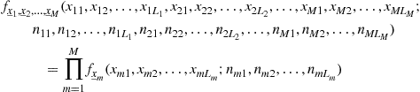 (4.102)
for any choice of time instants.
1.04.4.3 First- and second-order moments for random processes and sequences
It is not necessary to redefine moments in the context of random processes and sequences, since we will always be tackling a set of random variables as in Section 1.04.3.8. But it is useful to revisit the first- and second-order cases with a slightly modified notation to include time information.
For a random process ![]() , the following definitions apply:
, the following definitions apply:
As seen for random variables,
![]() (4.103)
(4.103)
which means that the mean instantaneous power of the process is the sum of a deterministic parcel with a random parcel.
Analogously, for a random sequence ![]() , the following definitions apply:
, the following definitions apply:
Again,
![]() (4.104)
(4.104)
i.e., the mean instantaneous power of the sequence is the sum of a deterministic parcel with a random parcel.
Given two random processes ![]() and
and ![]() , one defines:
, one defines:
The processes ![]() and
and ![]() are said to be mutually:
are said to be mutually:
The mean instantaneous power of ![]() is given by
is given by
![]() (4.105)
(4.105)
which suggests the definition of ![]() as the mean instantaneous cross power between
as the mean instantaneous cross power between ![]() and
and ![]() .
.
Analogously, given two random sequences ![]() and
and ![]() , one defines:
, one defines:
The sequences ![]() and
and ![]() are said to be mutually:
are said to be mutually:
The mean instantaneous power of ![]() is given by
is given by
![]() (4.106)
(4.106)
which suggests the definition of ![]() as the mean instantaneous cross power between
as the mean instantaneous cross power between ![]() and
and ![]() .
.
The interpretation of this “cross power” is not difficult: it accounts for the constructive or destructive interaction of the two involved processes (sequences) as dictated by their mutual correlation.
We will dedicate some space later to the properties of second-order moments.
1.04.4.4 Stationarity
The stationarity of random processes and sequences refers to the time-invariance of their statistical properties, which turns their treatment considerably easier.
Strict-sense is the strongest class of stationarity. A strict-sense stationary (SSS) random process ![]() (sequence
(sequence ![]() ) bears exactly the same statistical properties as
) bears exactly the same statistical properties as ![]() (
(![]() ), which means that its associated joint distribution for any set of time instants does not change when they are all shifted by the same time lag. A random process (sequence) in which each realization is a constant sampled from some statistical distribution in time is SSS.
), which means that its associated joint distribution for any set of time instants does not change when they are all shifted by the same time lag. A random process (sequence) in which each realization is a constant sampled from some statistical distribution in time is SSS.
Under this perspective, we can define that a random process ![]() is Lth-order stationary when
is Lth-order stationary when
![]() (4.107)
(4.107)
or, alternatively,
![]() (4.108)
(4.108)
Analogously, a random sequence ![]() is Lth-order stationary when
is Lth-order stationary when
![]() (4.109)
(4.109)
or, alternatively,
![]() (4.110)
(4.110)
We can say that an SSS random process or sequence is stationary for any order L. Moreover, Lth-order stationarity implies ![]() th-order stationarity, by marginalization at both sides of any of the four equations above.
th-order stationarity, by marginalization at both sides of any of the four equations above.
First-order stationarity says the statistical distribution at any individual instant of time t (n) is the same, i.e., ![]() does not depend on t (
does not depend on t (![]() does not depend on n). A natural consequence is the time-invariance of its statistical mean:
does not depend on n). A natural consequence is the time-invariance of its statistical mean: ![]()
![]() . Second-order stationarity says the joint statistical distribution at any two time instants t and
. Second-order stationarity says the joint statistical distribution at any two time instants t and ![]() for a fixed
for a fixed ![]() (n and
(n and ![]() for a fixed k) is the same. A natural consequence is the time-invariance of its auto-correlation, which can depend only of the time lag between the two time instants:
for a fixed k) is the same. A natural consequence is the time-invariance of its auto-correlation, which can depend only of the time lag between the two time instants: ![]()
![]() .
.
A weaker class of stationarity called wide-sense is much used in practice for its simple testability. A random process ![]() (sequence
(sequence ![]() ) is said to be wide-sense stationary (WSS) when its mean and auto-correlation are time-invariant. Such conditions do not imply stationarity of any order, although second-order stationarity implies wide-sense stationarity. As an extension of such definition, one says that two processes
) is said to be wide-sense stationary (WSS) when its mean and auto-correlation are time-invariant. Such conditions do not imply stationarity of any order, although second-order stationarity implies wide-sense stationarity. As an extension of such definition, one says that two processes ![]() and
and ![]() (sequences
(sequences ![]() and
and ![]() ) are jointly WSS when they are individually WSS and their cross-correlation is time-invariant, i.e., can depend only of the time lag between the two time instants:
) are jointly WSS when they are individually WSS and their cross-correlation is time-invariant, i.e., can depend only of the time lag between the two time instants: ![]()
![]() .
.
1.04.4.5 Properties of correlation functions for WSS processes and sequences
Wide-sense stationarity in random processes and sequences induces several interesting properties, some of which are listed below. For processes,
For sequences,
Even if the properties are not proven here, some interesting observations can be traced about them:
• The statistical behavior of the process (sequence) at a given instant of time is maximally correlated with itself, an intuitive result.
• The autocorrelation commutes.
• The statistical behaviors of a WSS process (sequence) with no periodic components at two time instants separated by ![]() are uncorrelated. Then, the autocorrelation tends to the product of two identical statistical means.
are uncorrelated. Then, the autocorrelation tends to the product of two identical statistical means.
• Periodic components in the process (sequence) cause the correlation maximum and surrounding behavior to repeat at each fundamental period.
• The arithmetic and geometric mean properties are in a certain sense linked to the first property. The second property is more stringent than the first.
1.04.4.6 Time averages of random processes and sequences
The proper use of random processes and sequences to model practical problems depends on the careful understanding of both their statistical and time variations. The main difference between these two contexts, which must be kept in mind, is the fact that time is inexorably ordered, thus allowing the inclusion in the model of some deterministic (predictable) time-structure. When we examine the statistical auto-correlation between two time instants of a random process or sequence, we learn how the statistical samples taken at those instants follow each other. In a WSS process or sequence, this measure for different lags can convey an idea of statistical periodicity.15 But what if one is concerned with the time structure and characteristics of each (or some) individual realization of a given process or sequence? The use of time averages can provide this complementary description.
The time average of a given continuous-time function ![]() can be defined as
can be defined as
![]() (4.111)
(4.111)
Given the random process ![]() , the time average of any of its realizations
, the time average of any of its realizations ![]() is
is
![]() (4.112)
(4.112)
The average power of ![]() is
is
![]() (4.113)
(4.113)
The time auto-correlation of ![]() for a lag
for a lag ![]() is defined as
is defined as
![]() (4.114)
(4.114)
The time cross-correlation between the realizations ![]() of process
of process ![]() and
and ![]() of process
of process ![]() for a lag
for a lag ![]() is defined as
is defined as
![]() (4.115)
(4.115)
As in the statistical case, an average cross power between ![]() and
and ![]() , which accounts for their mutual constructive or destructive interferences due to their time structure, can be defined as
, which accounts for their mutual constructive or destructive interferences due to their time structure, can be defined as
![]() (4.116)
(4.116)
Computed for the complete ensemble, such measures produce the random variables ![]() ,
, ![]() ,
, ![]() ,
, ![]() , and
, and ![]() , respectively. Under mild convergence conditions,
, respectively. Under mild convergence conditions,
![]() (4.117)
(4.117)
![]() (4.118)
(4.118)
![]() (4.119)
(4.119)
![]() (4.120)
(4.120)
![]() (4.121)
(4.121)
which are respectively the overall mean value, mean power, and auto-correlation (for lag ![]() ) of process
) of process ![]() , and cross-correlation (for lag
, and cross-correlation (for lag ![]() ) and mean cross power between processes
) and mean cross power between processes ![]() and
and ![]() .
.
The time average of a given discrete-time function ![]() can be defined as
can be defined as
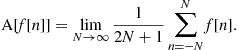 (4.122)
Given the random sequence ![]() , the time average of any of its realizations
, the time average of any of its realizations ![]() is
is
![]() (4.123)
(4.123)
The average power of ![]() is
is
![]() (4.124)
(4.124)
The time auto-correlation of ![]() for lag k is defined as
for lag k is defined as
![]() (4.125)
(4.125)
The time cross-correlation between the realizations ![]() of sequence
of sequence ![]() and
and ![]() of sequence
of sequence ![]() for lag k is defined as
for lag k is defined as
![]() (4.126)
(4.126)
As in the statistical case, an average cross power between ![]() and
and ![]() , which accounts for their mutual constructive or destructive interferences due to their time structure, can be defined as
, which accounts for their mutual constructive or destructive interferences due to their time structure, can be defined as
![]() (4.127)
(4.127)
Computed for the complete ensemble, such measures produce the random variables ![]() ,
, ![]() ,
, ![]() , and
, and ![]() , respectively. Under mild convergence conditions,
, respectively. Under mild convergence conditions,
![]() (4.128)
(4.128)
![]() (4.129)
(4.129)
![]() (4.130)
(4.130)
![]() (4.131)
(4.131)
and
![]() (4.132)
(4.132)
which are respectively the overall mean value, mean power, and auto-correlation (for lag k) of sequence ![]() , and cross-correlation (for lag k) and mean cross power between sequences
, and cross-correlation (for lag k) and mean cross power between sequences ![]() and
and ![]() .
.
As an example, consider that a deterministic signal ![]() (with
(with ![]() ) is additively contaminated by random noise
) is additively contaminated by random noise ![]() which can be modeled as a realization of the WSS random process
which can be modeled as a realization of the WSS random process ![]() (with
(with ![]() and
and ![]() ), thus yielding the random signal
), thus yielding the random signal ![]() . The corresponding process
. The corresponding process ![]() is obviously not WSS, since
is obviously not WSS, since ![]() . Furthermore, (following the nomenclature we have adopted) we can compute its:
. Furthermore, (following the nomenclature we have adopted) we can compute its:
Defining the signal-to-noise ratio (SNR) as the ratio between signal and noise powers, we can conclude that ![]() .
.
Now, suppose that two differently contaminated versions of ![]() are available:
are available: ![]() and
and ![]() , and that the underlying noise processes
, and that the underlying noise processes ![]() and
and ![]() are jointly WSS and uncorrelated, with
are jointly WSS and uncorrelated, with ![]() ,
, ![]() , and
, and ![]() . If an average signal
. If an average signal ![]() is computed, we can guarantee
is computed, we can guarantee ![]() and
and ![]() (i.e., noise is reduced) as long as
(i.e., noise is reduced) as long as ![]() .
.
1.04.4.7 Ergodicity
The so-called ergodicity is a property that allows interchanging statistic and temporal characteristics of some random processes (sequences)—which are then called ergodic. There are several levels of ergodicity, some of which are discussed below.
A random process ![]() with constant statistical mean is said to be mean-ergodic when any time average
with constant statistical mean is said to be mean-ergodic when any time average ![]() is equal to
is equal to ![]() with probability 1, which requires
with probability 1, which requires ![]() . If
. If ![]() is WSS, a necessary and sufficient condition for mean-ergodicity is
is WSS, a necessary and sufficient condition for mean-ergodicity is
![]() (4.133)
(4.133)
A random process ![]() with time-invariant auto-correlation is said to be auto-correlation-ergodic when any time auto-correlation
with time-invariant auto-correlation is said to be auto-correlation-ergodic when any time auto-correlation ![]() is equal to
is equal to ![]() with probability 1, which requires
with probability 1, which requires ![]() . Two processes
. Two processes ![]() and
and ![]() with time-invariant cross-correlation are cross-correlation-ergodic when any time cross-correlation
with time-invariant cross-correlation are cross-correlation-ergodic when any time cross-correlation ![]() is equal to
is equal to ![]() with probability 1, which requires
with probability 1, which requires ![]() . Conditions for correlation-ergodicity of random processes involve 4th-order moments.
. Conditions for correlation-ergodicity of random processes involve 4th-order moments.
A random sequence ![]() with constant statistical mean is said to be mean-ergodic when any time average
with constant statistical mean is said to be mean-ergodic when any time average ![]() is equal to
is equal to ![]() with probability 1, which requires
with probability 1, which requires ![]() . If
. If ![]() is WSS, a necessary and sufficient condition for mean-ergodicity is
is WSS, a necessary and sufficient condition for mean-ergodicity is
 (4.134)
A random sequence ![]() with time-invariant auto-correlation is said to be auto-correlation-ergodic when any time auto-correlation
with time-invariant auto-correlation is said to be auto-correlation-ergodic when any time auto-correlation ![]() is equal to
is equal to ![]() with probability 1, which requires
with probability 1, which requires ![]() . Two sequences
. Two sequences ![]() and
and ![]() with time-invariant cross-correlation are cross-correlation-ergodic when any time cross-correlation
with time-invariant cross-correlation are cross-correlation-ergodic when any time cross-correlation ![]() is equal to
is equal to ![]() with probability 1, which requires
with probability 1, which requires ![]() . Conditions for correlation-ergodicity of random sequences involve 4th-order moments.
. Conditions for correlation-ergodicity of random sequences involve 4th-order moments.
A process (sequence) that is mean- and auto-correlation-ergodic is called wide-sense ergodic. Two wide-sense ergodic processes (sequences) that are cross-correlation-ergodic are called jointly wide-sense ergodic.
A process (sequence) is distribution-ergodic when is ergodic for every moment.
The SSS random process (sequence) formed by random constant realizations is not ergodic in any sense. From Eqs. (4.133) and (4.134), a WSS process ![]() (sequence
(sequence ![]() ), statistically uncorrelated at any different time instants
), statistically uncorrelated at any different time instants ![]() and
and ![]() (
(![]() and
and ![]() ), i.e., with
), i.e., with ![]() (
(![]() ), is mean-ergodic.
), is mean-ergodic.
In practical real-life situations, quite often just a single realization of an underlying random process (sequence) is available. In such cases, if the latter is known to be ergodic, we can make use of the complete powerful statistical modeling framework described in this chapter. But how can one guarantee the property is enjoyed by a process (sequence) of which an only sample function is known? This is not so stringent a requirement: in fact, one needs just to be sure that there can be an ergodic process (sequence) of which that time function is a realization. Strictly speaking, a given music recording ![]() additively contaminated by background noise
additively contaminated by background noise ![]() cannot be modeled as a realization of a mean-ergodic process,16 since each member of the ensemble would combine the same
cannot be modeled as a realization of a mean-ergodic process,16 since each member of the ensemble would combine the same ![]() with a different
with a different ![]() . The random process which describes the noisy signal can be written as
. The random process which describes the noisy signal can be written as ![]() ; thus,
; thus, ![]() , while in practice we know that
, while in practice we know that ![]() .
.
1.04.4.8 An encompassing example
Define the random sequences ![]() and
and ![]() , such that:
, such that:
• ![]() is a random variable with mean
is a random variable with mean ![]() and variance
and variance ![]() ;
;
• ![]() is a random variable with mean
is a random variable with mean ![]() and variance
and variance ![]() ;
;
• ![]() rad/sample is a real constant;
rad/sample is a real constant;
• ![]() is a random variable uniformly distributed between
is a random variable uniformly distributed between ![]() and
and ![]() rad;
rad;
• ![]() is a random variable uniformly distributed between
is a random variable uniformly distributed between ![]() and
and ![]() rad;
rad;
Compute their time and statistical means, mean powers, auto-correlations, cross-correlations, and mean cross-powers; and discuss their correlation, orthogonality, stationarity, and ergodicity.
Solution 3
Time-averages:
![]() (4.135)
(4.135)
![]() (4.136)
(4.136)
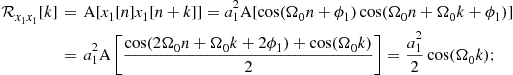 (4.137)
then,
![]() (4.138)
(4.138)
 (4.139)
then,
![]() (4.140)
(4.140)
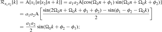 (4.141)
then,
![]() (4.142)
(4.142)
Expected values:
 (4.143)
 (4.144)
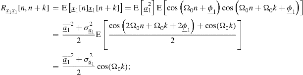 (4.145)
then,
![]() (4.146)
(4.146)
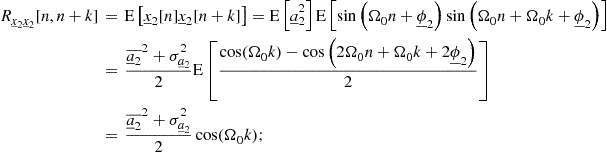 (4.147)
then,
![]() (4.148)
(4.148)
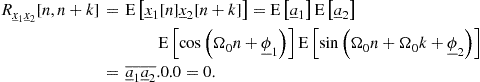 (4.149)
Conclusions:
1.04.4.9 Gaussian processes and sequences
A very special case of random processes (sequences) are the Gaussian-distributed. The corresponding Lth-order PDFs can be written (see Section 1.04.3.10).
 (4.150)
where ![]() is the
is the ![]() mean-vector with elements
mean-vector with elements ![]() , for
, for ![]() , and
, and ![]() is the
is the ![]() covariance-matrix with elements
covariance-matrix with elements ![]() , for
, for ![]() ;
;
 (4.151)
where ![]() is the
is the ![]() mean-vector with elements
mean-vector with elements ![]() , for
, for ![]() , and
, and ![]() is the
is the ![]() covariance-matrix with elements
covariance-matrix with elements ![]() , for
, for ![]() .
.
From the definition above:
• A WSS Gaussian random process (sequence) is SSS: Since the PDF of a Gaussian process (sequence) is entirely described by first- and second-order moments, if these moments do not depend on t (n), the PDF itself does not depend on t (n).
• Uncorrelated Gaussian processes (sequences) are independent: A joint PDF of two uncorrelated Gaussian processes (sequences) can be easily factorized as the product of their individual PDFs, since the covariance-matrix becomes block diagonal.
These two strong properties turn Gaussian models mathematically simpler to tackle, and the strict-sense stationarity and independence conditions easier to meet in practice.
The reader is invited to show that a stationary Gaussian process (sequence) whose auto-correlation is absolutely integrable in ![]() (summable in k) is ergodic.
(summable in k) is ergodic.
1.04.4.10 Poisson random process
Poisson is an example of discrete random process that we have already defined in Section 1.04.3.2. Each realization ![]() of
of ![]() counts the occurrences along time of a certain event whose mean occurrence rate is
counts the occurrences along time of a certain event whose mean occurrence rate is ![]() per time unit, provided that.
per time unit, provided that.
It can model the entry of clients in a store, for example. By convention:
Time origin can be shifted if necessary.
From Eq. (4.32), the first-order PDF of a Poisson process is given by
 (4.152)
Applying the definition iteratively, one can show that for ![]() , the corresponding Lth-order PDF is
, the corresponding Lth-order PDF is
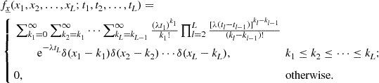 (4.153)
1.04.4.11 Complex random processes and sequences
Analogously to what has been done for random variables, real random processes and sequences can be generalized to handle the complex case.
A complex random process can be described as ![]() , where
, where ![]() and
and ![]() are real random processes. It is stationary in some sense as long as
are real random processes. It is stationary in some sense as long as ![]() e
e ![]() are jointly stationary in that sense. The remaining definitions related to process stationarity are kept the same.
are jointly stationary in that sense. The remaining definitions related to process stationarity are kept the same.
For a complex random process ![]() , the following definitions apply:
, the following definitions apply:
Given two random processes ![]() and
and ![]() , one defines:
, one defines:
The processes ![]() and
and ![]() are said to be mutually:
are said to be mutually:
For a random sequence ![]() , the following definitions apply:
, the following definitions apply:
Given two random processes ![]() and
and ![]() , one defines:
, one defines:
The processes ![]() and
and ![]() are said to be mutually:
are said to be mutually:
1.04.4.12 Markov chains
The simplest random processes (sequences) are those whose statistics at a given time are independent from every other time: a first-order distribution suffices to describe them. A less trivial model is found when the statistical time interdependency assumes a special recursive behavior such that the knowledge of a past conditioning state summarizes all previous history of the process (sequence). For the so-called Markov random process (sequence), the knowledge of the past does not affect the expectation of the future when the present is known.
Mathematically, a random process ![]() is said to be a Markov process when for
is said to be a Markov process when for ![]() ,
,
![]() (4.154)
(4.154)
or for ![]() ,
,
![]() (4.155)
(4.155)
We will restrict ourselves to the discrete-time case. A random sequence ![]() is said to be a Markov sequence when
is said to be a Markov sequence when
![]() (4.156)
(4.156)
which can be seen as a transition PDF. From the definition, one arrives at the chain rule
![]() (4.157)
(4.157)
which means that the overall Markov sequence can be statistically described for ![]() from the knowledge of its distribution at
from the knowledge of its distribution at ![]() and its subsequent transition distributions. Some interesting properties can be deduced from the expressions above:
and its subsequent transition distributions. Some interesting properties can be deduced from the expressions above:
A much important property of Markov sequences is the so-called Chapman-Kolmogorov equation: for ![]() ,
,
![]() (4.158)
(4.158)
which provides a recursive way to compute arbitrary transition PDFs.
We can say a Markov sequence ![]() is stationary when
is stationary when ![]() and
and ![]() are shift-invariant. In this case, the overall sequence can be obtained from
are shift-invariant. In this case, the overall sequence can be obtained from ![]() . A less trivial (and quite useful) model is provided by homogeneous Markov sequences, which are characterized only by a shift-invariant transition distribution; they are not stationary in general, but can be asymptotically stationary (i.e., for
. A less trivial (and quite useful) model is provided by homogeneous Markov sequences, which are characterized only by a shift-invariant transition distribution; they are not stationary in general, but can be asymptotically stationary (i.e., for ![]() ) under certain conditions.
) under certain conditions.
Discrete Markov processes and sequences are called Markov chains, which can assume a countable number of random states ![]() described by their state probabilities (
described by their state probabilities (![]() for sequences) and transition probabilities (
for sequences) and transition probabilities (![]() for sequences). Discrete-time Markov chains enjoy the following properties, for
for sequences). Discrete-time Markov chains enjoy the following properties, for ![]() :
:
• ![]() , which totalizes all possible ways to left state
, which totalizes all possible ways to left state ![]() in
in ![]() ;
;
• ![]() , which totalizes all possible ways to arrive at state
, which totalizes all possible ways to arrive at state ![]() in
in ![]() ;
;
If the chain has a finite number of states, a matrix notation can be employed. The state probability vector ![]() , with elements
, with elements ![]() , and the transition probability matrix
, and the transition probability matrix ![]() , with elements
, with elements ![]() , are related by
, are related by ![]() .
.
The special class of homogeneous Markov chains enjoys the following additional properties:
Accordingly, the transition probability matrix becomes ![]() . Defining
. Defining ![]() ,
,
![]() (4.159)
(4.159)
i.e., ![]() . When asymptotic stationarity is reachable, one can find the steady-state probability vector
. When asymptotic stationarity is reachable, one can find the steady-state probability vector![]() such that
such that ![]() .
.
Consider, for example, the homogeneous Markov chain ![]() depicted in Figure 4.12, with states 1 and 2, state probabilities
depicted in Figure 4.12, with states 1 and 2, state probabilities ![]() and
and ![]() , and transition probabilities
, and transition probabilities ![]() and
and ![]() . Its corresponding one-sample transition matrix is
. Its corresponding one-sample transition matrix is
 (4.160)
such that
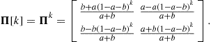 (4.161)
It can also be shown that the chain reaches the steady-state probability vector
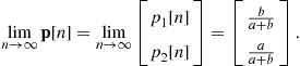 (4.162)

1.04.4.13 Spectral description of random processes and sequences
At first sight, the direct conversion of each realization ![]() (
(![]() ) to the frequency domain seems the easiest way to spectrally characterize a random process
) to the frequency domain seems the easiest way to spectrally characterize a random process ![]() (sequence
(sequence ![]() ). However, it is difficult to guarantee the existence of the Fourier transform
). However, it is difficult to guarantee the existence of the Fourier transform
![]() (4.163)
(4.163)
(in the case os random processes) or
![]() (4.164)
(4.164)
(in the case of random sequences) for every realization. And even if possible, we would get a random spectrum of limited applicability. In Section 1.04.4.5, we have found that the auto-correlation conveys information about every sinusoidal component found in the process (sequence). A correct interpretation of the Fourier transform17 suggests that the auto-correlation in fact conveys information about the overall spectrum of the process (sequence). Furthermore, it is a better behaved function than the individual realizations, and thus amenable to be Fourier transformed.
In Section 1.04.4.6, Eq. (4.118), we defined the overall mean power of the random process ![]() , which for the general complex case, becomes
, which for the general complex case, becomes
![]() (4.165)
(4.165)
It can be shown that
![]() (4.166)
(4.166)
where
![]() (4.167)
(4.167)
and
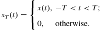 (4.168)
We can then define a power spectral density
![]() (4.169)
(4.169)
such that ![]() . Some additional algebraic manipulation yields
. Some additional algebraic manipulation yields
![]() (4.170)
(4.170)
which directly relates the auto-correlation to the power spectral density of the process, as predicted. From the expressions above, ![]() is a non-negative real function of
is a non-negative real function of ![]() . Furthermore, if
. Furthermore, if ![]() is real, then
is real, then ![]() is an even function of
is an even function of ![]() .
.
In Section 1.04.4.6, Eq. (4.121), we also defined the overall mean cross-power between the processes ![]() and
and ![]() , which for the general complex case, becomes
, which for the general complex case, becomes
![]() (4.171)
(4.171)
Following the same steps as above, we arrive at
![]() (4.172)
(4.172)
where ![]() is defined as before,
is defined as before,
![]() (4.173)
(4.173)
and
 (4.174)
We can then define the corresponding cross-power spectral density
![]() (4.175)
(4.175)
such that ![]() . In terms of the cross-correlation, the cross-power spectral density can be written as
. In terms of the cross-correlation, the cross-power spectral density can be written as
![]() (4.176)
(4.176)
As expected, the cross-power density of orthogonal processes is zero. From the expressions above, ![]() . Furthermore, if
. Furthermore, if ![]() and
and ![]() are real, then the real part of
are real, then the real part of ![]() is even and the imaginary part of
is even and the imaginary part of ![]() is odd.
is odd.
It should be noticed that in the WSS case, ![]() ,
, ![]() ,
, ![]() , and
, and ![]() .
.
A similar development can be done for random sequences. In Section 1.04.4.6, Eq. (4.129), we defined the overall mean power of the random sequence ![]() , which for the general complex case, becomes
, which for the general complex case, becomes
![]() (4.177)
(4.177)
It can be shown that
![]() (4.178)
(4.178)
where
![]() (4.179)
(4.179)
and
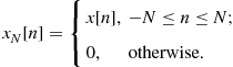 (4.180)
We can then define a power spectral density
![]() (4.181)
(4.181)
such that ![]() . Some additional algebraic manipulation yields
. Some additional algebraic manipulation yields
![]() (4.182)
(4.182)
which directly relates the auto-correlation to the power spectral density of the random sequence, as expected. From the expressions above, ![]() is a non-negative real function of
is a non-negative real function of ![]() . Furthermore, if
. Furthermore, if ![]() is real, then
is real, then ![]() is an even function of
is an even function of ![]() .
.
In Section 1.04.4.6, Eq. (4.132), we also defined the overall mean cross-power between the random sequences ![]() and
and ![]() , which for the general complex case, becomes
, which for the general complex case, becomes
![]() (4.183)
(4.183)
Following the same steps as above, we arrive at
![]() (4.184)
(4.184)
where ![]() is defined as before,
is defined as before,
![]() (4.185)
(4.185)
and
 (4.186)
We can then define the corresponding cross-power spectral density
![]() (4.187)
(4.187)
such that ![]() . In terms of the cross-correlation, the cross-power spectral density can be written as
. In terms of the cross-correlation, the cross-power spectral density can be written as
![]() (4.188)
(4.188)
As expected, the cross-power density of orthogonal processes is zero. From the expressions above, ![]() . Furthermore, if
. Furthermore, if ![]() and
and ![]() are real, then the real part of
are real, then the real part of ![]() is even and the imaginary part of
is even and the imaginary part of ![]() is odd.
is odd.
1.04.4.14 White and colored noise
One usually refers to a disturbing signal ![]()
![]() as noise. Since noise signals are typically unpredictable, they are preferably modeled as realizations of some noise random process
as noise. Since noise signals are typically unpredictable, they are preferably modeled as realizations of some noise random process ![]() (sequence
(sequence ![]() ).
).
A very special case is the so-called white noise (by analogy with white light), which is a uniform combination of all frequencies.
Continuous-time white noise ![]() is sampled from a random process
is sampled from a random process ![]() characterized by the following properties:
characterized by the following properties:
From the last property, continuous-time white noise is not physically realizable. Furthermore, WSS continuous-time white noise has ![]() .
.
Discrete-time white noise ![]() is sampled from a random sequence
is sampled from a random sequence ![]() characterized by the following properties:
characterized by the following properties:
For WSS discrete-time white noise, ![]() ,
, ![]() , and
, and ![]() .
.
Unless differently stated, white noise is implicitly assumed to be generated by a WSS random process (sequence). Notice, however, that the sequence ![]() , where
, where ![]() rad and
rad and ![]() is WSS white noise with unit variance, for example, satisfies all conditions to be called white noise, even if
is WSS white noise with unit variance, for example, satisfies all conditions to be called white noise, even if ![]() .
.
A common (more stringent) model of white noise imposes that values at different time instants of the underlying process (sequence) be statistically i.i.d.
Any random noise whose associated power spectral density is not constant is said to be colored noise. One can find in the literature several identified colored noises (pink, grey, etc.), each one with a pre-specified spectral behavior. It should also be noticed that any band-limited approximation of white noise destroys its non-correlation property. Consider ![]() generated by a WSS random process
generated by a WSS random process ![]() such that
such that
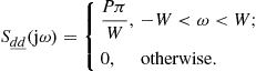 (4.189)
It is common practice to call ![]() “white noise” of bandwidth W and overall mean power P. Since its auto-correlation is
“white noise” of bandwidth W and overall mean power P. Since its auto-correlation is
![]() (4.190)
(4.190)
1.04.4.15 Applications: modulation, “Bandpass” and band-limited processes, and sampling
An interesting application of the spectral description of random processes is modeling of AM (amplitude modulation). Assuming a carrier signal ![]() modulated by a real random signal
modulated by a real random signal ![]() sampled from a process
sampled from a process ![]() , the resulting modulated random process
, the resulting modulated random process ![]() has auto-correlation
has auto-correlation
![]() (4.191)
(4.191)
If ![]() is WSS, then
is WSS, then
![]() (4.192)
(4.192)
and the corresponding power spectral density is
![]() (4.193)
(4.193)
We conclude that the AM constitution of ![]() carries through its auto-correlation, which provides a simple statistical model for AM.
carries through its auto-correlation, which provides a simple statistical model for AM.
Quite often we find ourselves dealing with band-limited random signals. In the AM discussion above, typically ![]() has bandwidth
has bandwidth ![]() . For a random process
. For a random process ![]() whose spectrum is at least concentrated around
whose spectrum is at least concentrated around ![]() (baseband process), we can attribute it an RMS (root-mean-squared) bandwidth
(baseband process), we can attribute it an RMS (root-mean-squared) bandwidth![]() such that
such that
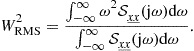 (4.194)
If the spectrum is concentrated around a centroid
![]() (4.195)
(4.195)
![]() is given by
is given by
 (4.196)
If the process bandwidth excludes ![]() , it is called18 a “bandpass” process.
, it is called18 a “bandpass” process.
It can be shown that if a band-limited baseband WSS random process ![]() with bandwidth W, i.e., such that
with bandwidth W, i.e., such that ![]() for
for ![]() , is sampled at rate
, is sampled at rate ![]() to generate the random sequence
to generate the random sequence
![]() (4.197)
(4.197)
then ![]() can be recovered from
can be recovered from ![]() with zero mean-squared-error. This is the stochastic version of the Nyquist criterion for lossless sampling.
with zero mean-squared-error. This is the stochastic version of the Nyquist criterion for lossless sampling.
1.04.4.16 Processing of random processes and sequences
Statistical signal modeling is often employed in the context of signal processing, and thus the interaction between random signals and processing systems calls for a systematic approach. In this chapter, we will restrict ourselves to linear time-invariant (LTI) systems.
A system defined by the operation ![]() between input x and output y is called linear if any linear combination of m inputs produce as output the same linear combination of their m corresponding outputs:
between input x and output y is called linear if any linear combination of m inputs produce as output the same linear combination of their m corresponding outputs:
For a linear system, one can define an impulse response h as the system output to a unit impulse ![]() applied to the system input at a given time instant:
applied to the system input at a given time instant:
• for a continuous-time system, a unit impulse ![]() applied at instant
applied at instant ![]() , produces an impulse response
, produces an impulse response ![]() ,
,
• for a discrete-time system, a unit impulse19![]() applied at instant k, produces an impulse response
applied at instant k, produces an impulse response ![]() .
.
A system is called time-invariant if a given input x applied at different time instants produces the same output y accordingly time-shifted:
The output of an LTI system to any input x is the convolution![]() between the input and the impulse response h of the system:
between the input and the impulse response h of the system:
In the frequency domain, the output Y is related to the input X by the system frequency response H:
The product XH brings the concept of filtering: H defines how much of each frequency component of input X passes to the output Y. From now on, when referring to the processing of a random process (sequence) by a system we imply that each process realization is filtered by that system.
The filtering of a random process ![]() by an LTI system with impulse response
by an LTI system with impulse response ![]() results in another random process
results in another random process ![]() such that
such that ![]() . Assuming
. Assuming ![]() WSS and possibly complex, so as
WSS and possibly complex, so as ![]() , then
, then ![]() will be also WSS and20:
will be also WSS and20:
The processing of a random sequence ![]() by an LTI system with impulse response
by an LTI system with impulse response ![]() results in another random sequence
results in another random sequence ![]() such that
such that ![]() . Assuming
. Assuming ![]() WSS and possibly complex, so as
WSS and possibly complex, so as ![]() , then
, then ![]() will be also WSS and21:
will be also WSS and21:
Among the above results, one of the most important is the effect of filtering on the power spectral density ![]() of the input WSS random process (sequence): it is multiplied by the squared magnitude
of the input WSS random process (sequence): it is multiplied by the squared magnitude ![]() of the frequency response of the LTI system to produce the power spectral density
of the frequency response of the LTI system to produce the power spectral density ![]() of the output WSS random process (sequence). As a direct consequence, any WSS random process (sequence) with known power spectral density S can be modeled by the output of an LTI system with squared magnitude response
of the output WSS random process (sequence). As a direct consequence, any WSS random process (sequence) with known power spectral density S can be modeled by the output of an LTI system with squared magnitude response ![]() whose input is white noise.
whose input is white noise.
In order to qualitatively illustrate this filtering effect:
• Figure 4.13 shows 200 samples of white noise ![]() ;
;
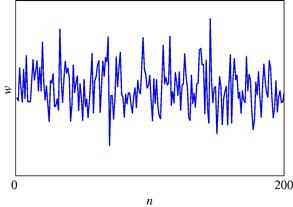
• Figure 4.14 shows 200 samples of ![]() , a slowly evolving signal obtained by low-pass filtering of
, a slowly evolving signal obtained by low-pass filtering of ![]() to 20% of its original bandwidth;
to 20% of its original bandwidth;
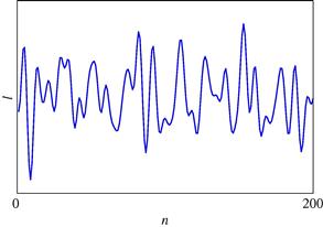
• Figure 4.15 shows 200 samples of ![]() , an almost sinusoidal signal obtained by band-pass filtering of
, an almost sinusoidal signal obtained by band-pass filtering of ![]() to the central 4% of its original bandwidth.
to the central 4% of its original bandwidth.
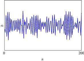
From the area of optimum filtering, whose overall goal is finding the best filter to perform a defined task, we can bring an important application of the concepts presented in this section. The general discrete Wiener filter H, illustrated in Figure 4.16, is the linear time-invariant filter which minimizes the mean quadratic value ![]() of the error
of the error ![]() between the desired signal
between the desired signal ![]() and the filtered version
and the filtered version ![]() of the input signal
of the input signal ![]() . Assuming that
. Assuming that ![]() and
and ![]() are realizations of two jointly WSS random sequences
are realizations of two jointly WSS random sequences ![]() and
and ![]() , if the optimum filter is not constrained to be causal, one finds that it must satisfy the equation
, if the optimum filter is not constrained to be causal, one finds that it must satisfy the equation
![]() (4.198)
(4.198)
i.e., its frequency response is
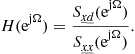 (4.199)
If one needs a causal FIR solution, a different but equally simple solution can be found for ![]() .
.
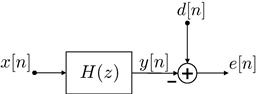
We can solve a very simple example where we compute an optimum zero-order predictor for a given signal of which a noisy version is available. In this case, ![]() (a simple gain to be determined), the input
(a simple gain to be determined), the input ![]() (signal
(signal ![]() additively corrupted by noise
additively corrupted by noise ![]() ) and
) and ![]() . The solution is
. The solution is
![]() (4.200)
(4.200)
which yields the minimum mean quadratic error
 (4.201)
Notice that if no noise is present,
![]() (4.202)
(4.202)
and
![]() (4.203)
(4.203)
The reader should be aware that this example studies a theoretical probabilistic model, which may therefore depend on several parameters which probably would not be available in practice and should rather be estimated. In fact, it points out the solution a practical system should pursue.
The Wiener filter is a kind of benchmark for adaptive filters [7], which optimize themselves recursively.
1.04.4.17 Characterization of LTI systems and WSS random processes
A direct way to find the impulse response ![]() of an LTI system is to apply white noise
of an LTI system is to apply white noise ![]() with power spectral density
with power spectral density ![]() to the system input, which yields
to the system input, which yields ![]() . From an estimate
. From an estimate ![]() of the cross-correlation, one can obtain an estimate of the desired impulse response:
of the cross-correlation, one can obtain an estimate of the desired impulse response: ![]() . In practice, assuming ergodicity, the following approximations are employed:
. In practice, assuming ergodicity, the following approximations are employed:
Furthermore, the operations are often performed in the discrete-time domain.
The effective bandwidth of an LTI system with frequency response ![]() can be estimated by its noise bandwidth
can be estimated by its noise bandwidth![]() . For a low-pass system, one looks for an equivalent ideal low-pass filter with bandwidth
. For a low-pass system, one looks for an equivalent ideal low-pass filter with bandwidth ![]() around
around ![]() with bandpass gain
with bandpass gain ![]() ;
; ![]() is computed to guarantee that both systems deliver the same mean output power when the same white noise is applied to their both inputs. A straightforward algebraic development yields
is computed to guarantee that both systems deliver the same mean output power when the same white noise is applied to their both inputs. A straightforward algebraic development yields
![]() (4.204)
(4.204)
For a band-pass system with magnitude response centered about ![]() , one looks for an ideal band-pass filter equivalent with bandwidth
, one looks for an ideal band-pass filter equivalent with bandwidth ![]() around
around ![]() with bandpass gain
with bandpass gain ![]() is computed to guarantee that both systems delivers the same mean output power when the same equal white noise is applied to their both inputs. For this case,
is computed to guarantee that both systems delivers the same mean output power when the same equal white noise is applied to their both inputs. For this case,
![]() (4.205)
(4.205)
A real “bandpass” random process (see Section 1.04.4.15) about center frequency ![]() can be expressed as
can be expressed as ![]() , where the envelope
, where the envelope ![]() and the phase
and the phase ![]() are both baseband random processes. We can write
are both baseband random processes. We can write
![]() (4.206)
(4.206)
where ![]() and
and ![]() are the quadrature components of
are the quadrature components of ![]() . In the typical situation where
. In the typical situation where ![]() is a zero-mean WSS random process with auto-correlation
is a zero-mean WSS random process with auto-correlation ![]() , we can explicitly find the first and second-order moments of the quadrature components that validate the model. First define the Hilbert transform of a given signal
, we can explicitly find the first and second-order moments of the quadrature components that validate the model. First define the Hilbert transform of a given signal ![]() as
as ![]() , where
, where
 (4.207)
From ![]() , we can find
, we can find ![]() and proceed to write:
and proceed to write:
In the frequency domain, if we define
 (4.208)
then
In the particular case where ![]() is Gaussian, it can be shown that
is Gaussian, it can be shown that ![]() and
and ![]() are Gaussian, and thus completely defined by their first- and second-order moments above.
are Gaussian, and thus completely defined by their first- and second-order moments above.
1.04.4.18 Statistical modeling of signals: random sequence as the output of an LTI system
A discrete-time signal ![]() with spectrum
with spectrum ![]() can be modeled as the output of a linear time-invariant system whose frequency response is equal to
can be modeled as the output of a linear time-invariant system whose frequency response is equal to ![]() when excited by a unit impulse
when excited by a unit impulse ![]() . In this case, the impulse response of the system is expected to be
. In this case, the impulse response of the system is expected to be ![]() .
.
In the context of statistic models, an analogous model can be built: now, we look for a linear time-invariant system which produces at its output the WSS random sequence ![]() with power spectral density
with power spectral density ![]() , when excited by a unit-variance random sequence
, when excited by a unit-variance random sequence ![]() of white noise. As before, the frequency response of the system alone is expected to shape the output spectrum, yet this time in the mean power sense, i.e., the system must be such that
of white noise. As before, the frequency response of the system alone is expected to shape the output spectrum, yet this time in the mean power sense, i.e., the system must be such that ![]() .
.
Assume the overall modeling system is described by the difference equation
![]() (4.209)
(4.209)
where ![]() is white noise with
is white noise with ![]() . The corresponding transfer function is
. The corresponding transfer function is
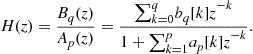 (4.210)
The output ![]() of this general system model with
of this general system model with ![]() at its input is called ARMA (auto-regressive moving-average22) process of order
at its input is called ARMA (auto-regressive moving-average22) process of order ![]() . It can be described by the following difference equation in terms of its auto-correlation:
. It can be described by the following difference equation in terms of its auto-correlation:
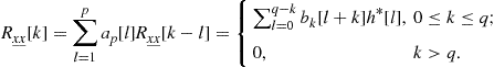 (4.211)
The values of ![]() for
for ![]() can be easily found by symmetry.
can be easily found by symmetry.
If one restricts the system to be FIR (i.e., to have a finite-duration impulse response), then ![]() , i.e.,
, i.e., ![]() for
for ![]() , and
, and
![]() (4.212)
(4.212)
The output of this “all-zero”23 system model with ![]() at its input is called an MA (moving-average) process of order q. Its auto-correlation can be found to be
at its input is called an MA (moving-average) process of order q. Its auto-correlation can be found to be
 (4.213)
In this case, ![]() for
for ![]() or
or ![]() . This model is more suited for modeling notches in the random sequence power spectrum.
. This model is more suited for modeling notches in the random sequence power spectrum.
If one restricts the system to be “all-pole,”24 then ![]() , i.e.,
, i.e., ![]() for
for ![]() , and
, and
![]() (4.214)
(4.214)
The output of this system model with ![]() at its input is called an AR (auto-regressive) process of order p. Its auto-correlation follows the difference equation below:
at its input is called an AR (auto-regressive) process of order p. Its auto-correlation follows the difference equation below:
 (4.215)
Again, the values of ![]() for
for ![]() can be easily found by symmetry. This model is more suited for modeling peaks in the random sequence power spectrum, which is typical of quasi-periodic signals (as audio signals, for example). It should be noticed that, differently from the ARMA and MA cases, the equation for the AR process auto-correlation is linear in the system coefficients, which makes their estimation easier. If
can be easily found by symmetry. This model is more suited for modeling peaks in the random sequence power spectrum, which is typical of quasi-periodic signals (as audio signals, for example). It should be noticed that, differently from the ARMA and MA cases, the equation for the AR process auto-correlation is linear in the system coefficients, which makes their estimation easier. If ![]() is known for
is known for ![]() , and recalling that
, and recalling that ![]() , one can:
, one can:
• solve the pth-order linear equation system obtained by substituting ![]() in Eq. (4.215) to find
in Eq. (4.215) to find ![]() ;
;
• compute ![]() from Eq. (4.215) with
from Eq. (4.215) with ![]() .
.
All-pole modeling of audio signals is extensively used in restoration systems [8].
Relevant Theory: Signal Processing Theory
References
1. Deep R. Probability and Statistics. San Diego: Academic; 2006.
2. Casella G, Berger RL. Statistical Inference. second ed. Pacific Grove: Duxbury; 2001.
3. Papoulis A, Unnikrishna P. Probability, Random Variables and Stochastic Processes. fourth ed. New York: McGraw-Hill; 2002.
4. Peebles Jr PZ. Probability, Random Variables and Random Signal Principles. fourth ed. New York: McGraw-Hill; 2001.
5. Shanmugan KS, Breipohl AM. Random Signals: Detection, Estimation and Data Analysis. New York: Wiley; 1988.
6. Hayes MH. Statistical Digital Signal Processing and Modeling. Hoboken: Wiley; 1996.
7. Diniz PSR. Adaptive Filtering: Algorithms and Practical Implementation. New York: Springer; 2012.
8. Godsill SJ, Rayner JW. Digital Audio Restoration: A Statistical Model Based Approach. London: Springer; 1988.
1Of course, other independent variables (e.g., space) can substitute for time in this context.
2Even if the literature sometimes prefers to employ “stochastic” for processes and “random” for signals, the expression “random processes” became common use and will be used throughout the chapter.
3One could think of mixed cases, but this discussion is better conveyed in the random variable framework, which comprises every possible mapping from the original experiment to a subset of the real numbers.
4Unit step function: 
5Unit impulse distribution, or Dirac delta: For ![]() and
and ![]() .
.
6This unusual notation is employed here for the sake of compatibility with the other definitions.
7Notice that the expected value of a random variable is not necessarily meaningful for the associated experiment.
8The classical definition does not subtracts three.
9Convolution integral: ![]() .
.
10Equation (4.43) can be seen as the next expression computed for ![]() , since
, since ![]() and
and ![]() .
.
11We will tackle only scalar parameters, without loss of generality.
12For the sake of simplicity, we refer only to the estimation of a fixed parameter ![]() .
.
13There are other definitions of consistence.
14In this text, for completeness we opted for always explicitly writing both formulations, for processes and sequences.
15We hinted this point when discussing the properties of second-order moments, in Section 1.04.4.5.
16Even if the author has done so many times.
17The Fourier transform represents a time signal as a linear combination of continuously distributed sinusoids.
18With considerable freedom of nomenclature.
19Unit impulse function, or Kronecker delta: For ![]() , and
, and ![]() .
.
20Where notation ![]() was used.
was used.
21Where notation ![]() was used.
was used.
22Auto-regressive for its output feedback, moving average for its weighted sum of past input samples.
23This is a misname, since the poles of the system are at the origin. In fact, the zeros are the only responsible for shaping the frequency response of the system.
24This is another misname, since the zeros of the system are at the origin. In fact, the poles are the only responsible for shaping the frequency response of the system.