
Online Learning in Reproducing Kernel Hilbert Spaces
Konstantinos Slavakis*, Pantelis Bouboulis† and Sergios Theodoridis†, *University of Peloponnese, Department of Telecommunications Science and Technology, Karaiskaki St., Tripolis 22100, Greece, †University of Athens, Department of Informatics and Telecommunications, Ilissia, Athens 15784, Greece
Abstract
Online learning has been at the center of focus in signal processing learning tasks for many decades, since the early days of the LMS and Kalman filtering and it has already found its place in a wide range of diverse applications and practical systems. More recently, together with the birth of new disciplines, such as information retrieval and bioinformatics, a new necessity for online learning techniques has emerged. The number of the available data as well as the dimensionality of the involved spaces can become excessively large for what batch processing techniques can cope with. In batch processing, all data have to be known prior to the start of the learning process and have to be stored in the memory. This is also true for batch techniques that use the data sequentially. In the online techniques to be described in this chapter, every data point is used only for a limited number of times. Besides their computational advantages, such techniques can easily accommodate modifications so that to deal with time varying statistics and produce estimates that can adapt to such variations. This is the reason that such techniques are also known as adaptive or time-adaptive techniques, especially in the signal processing community jargon.
As it is most often the case, when an application has a multidisciplinary flavor, a number of contributors, with a different background and experience, yet working on similar, if not the same, tasks, are involved who may be using different names and sometimes not referring to each other. Information retrieval and bioinformatics are such typical examples. One of the goals of this current chapter was to search within different communities and try to systematize, to the extend possible, various online schemes that have appeared and try to put them under a common umbrella.
Moreover, since the world of machine learning is not the same as it used to be before the SVM “era,” we have developed all our setting in general Reproducing Kernel Hilbert spaces (RKHS), and we have also tried to provide some brief historical review of this powerful mathematical tool as well as some basic definitions and properties, for the sake of completeness. It is worth pointing out that although in a wide range of machine learning tasks, such as pattern recognition, RKHS spaces have been widely adopted, the signal processing community, in spite of its very rich history and experience with nonlinear processing from the early days of Gabor and Wiener, still has been very reluctant to adopt such techniques. Another goal of this chapter is to make such techniques more familiar to this community, especially in their online/adaptive face, which is something that this community cares a lot.
The chapter focuses on parametric learning, serving the needs of both, pattern recognition and regression tasks, since these are the two main directions of modeling learning tasks that embrace a large number of applications.
We made an effort to build up the chapter with an increasing level of mathematical complexity. Starting from the simpler techniques and moving to the ones, which although they are simple to implement, their derivation needs mathematical tools that go beyond the standard university level curriculum courses. We have made an effort to use a lot of geometry in order to provide some further “physical” understanding of these methods, hence the reader, who is not interested in proofs, to be able to grasp the basic reasoning that runs across their spine.
Keywords
Online learning; Adaptive signal processing; Reproducing kernels; Hilbert spaces; Convexity; Metric projections; Proximal mappings; Nonexpansive mappings; Fixed point theory
Nomenclature
Training Data A set of input-output measurements that are used to train a specific learning machine
Online Learning A learning task, where the data points arrive sequentially and used only once
Batch Learning A learning task, where the training data are known beforehand
Regression Task A learning task that estimates a parametric input-output relationship that best fits the available data
Classification Task A learning task that classifies the data into one or more classes
Overfitting A common notion in the Machine Learning literature. If the adopted model is too complex then the learning algorithm tends to fit to the training data as much as possible (e.g., it fits even the noisy data) and cannot perform well when new data arrive
Regularization A technique that biases the solution towards a smoother result. This is usually achieved by adding the norm of the solution to the cost function of the minimization task
Sparsification A method that biases the solution towards a result, that the least significant components are pushed to zero
Reproducing Kernel Hilbert Spaces (RKHS) An inner product space of functions that is complete and has a special structure
Kernel A positive definite function of two variables that is associated to a specific RKHS
Fréchet Differentiation A mathematical framework that generalizes the notion of the standard derivative, to more general function spaces
Least Mean Squares This is a class of stochastic online learning tasks, which aim to find the parameters of an input-output relation by minimizing the least mean squares of the error at each iteration (difference between the desired and the actual output), using a gradient descent rationale
Recursive Least Squares A class of deterministic online learning tasks, which aim to find the parameters of an input-output relation by minimizing the least mean squares of the total error (the sum of differences between the desired and the actual output up to the current iteration) using a recursive Newton-like method
Adaptive Projected Subgradient Method (APSM) A convex analytic framework for online learning. Based on set theoretic estimation arguments, and fixed point theory, the APSM is tailored to attack online learning problems related to general, convexly constrained, non-smooth optimization tasks
Wirtinger’s Calculus A methodology for computing gradients of real valued functions that are defined on complex domains, using the standard rules of differentiation
1.17.1 Introduction
A large class of Machine Learning tasks becomes equivalent with estimating an unknown functional dependence that relates the so called input (cause) to the output (effect) variables. Most often, this function is chosen to be of a specific type, e.g., linear, quadratic, etc., and it is described by a set of unknown parameters. There are two major paths in dealing with this set of parameters.
The first one, known as Bayesian Inference, treats the parameters as random variables, [1]. According to this approach, the dependence between the input and output variables is expressed via a set of pdfs. The task of learning is to obtain estimates of the pdf that relates the input-output variables as well as the pdf that describes the random nature of the parameters. However, the main concern of the Bayesian Inference approach is not in obtaining specific values for the parameters. Bayesian Inference can live without this information. In contrast, the alternative path, which will be our focus in this paper, considers the unknown parameters to be deterministic and its major concern is to obtain specific estimates for their values.
Both trends share a common trait; they dig out the required information, in order to build up their estimates, from an available set of input-output measurements known as the training set. The stage of estimating the pdfs/parameters is known as training and this philosophy of learning is known as supervised learning. This is not the only approach which Machine Learning embraces in order to “learn” from data. Unsupervised and semi-supervised learning are also major learning directions, [2]. In the former, no measurements of the output variable(s) are available in the training data set. In the latter, there are only a few. In this paper, we will focus on the supervised learning of a set of deterministically treated parameters. We will refer to this task as parameter estimation.
In the parameter estimation task, depending on the adopted functional dependence, different models result. At this point, it has to be emphasized that the only “truth” that the designer has at his/her disposal is the set of training data. The model that the designer attempts to “fit” in the data is just a concept in an effort to be able to exploit and use the available measurements for his/her own benefit; that is, to be able to make useful predictions of the output values in the future, when new measurements of the inputs, outside the training set, become available. The ultimate goal of the obtained predictions is to assist the designer to make decisions, once the input measurements are disclosed to him/her. In nature, one can never know if there is a “true” model associated with the data. Our confidence in “true” models only concerns simulated data. In real life, one is obliged to adopt a model and a training method to learn its parameters so that the resulting predictions can be useful in practice. The designed Machine Learning system can be used till it is substituted by another, which will be based on a new model and/or a new training method, that leads to improved predictions and which can be computed with affordable computational resources.
In this paper, we are concerned with the more general case of nonlinear models. Obviously, different nonlinearities provide different models. Our approach will be in treating a large class of nonlinearities, which are usually met in practice, in a unifying way by mobilizing the powerful tool of Reproducing Kernel Hilbert Spaces (RKHS). This is an old concept, that was gradually developed within the functional analysis discipline [3] and it was, more recently, popularized in Machine Learning in the context of Support Vector Machines. This methodology allows one to treat a wide class of different nonlinearities in a unifying way, by solving an equivalent linear task in a space different than the one where the original measurements lie. This is done by adopting an implicit mapping from the input space to the so called feature space. In the realm of RKHSs, one needs not to bother about the specific nature of this space, not even about its dimensionality. Once the parametric training has been completed, the designer can “try” different implicit mappings, which correspond to different nonlinearities and keep the one that fits best his/her needs. This is achieved during the so-called validation stage. Ideally, this can be done by testing the performance of the resulting estimator using a data set that is independent of the one used for training. In case this is not possible, then various techniques are available in order to exploit a single data set, both for training and validation, [2].
Concerning the estimation process, once a parametric modeling has been adopted, the parameter estimation task relies on adopting, also, a criterion that measures the quality of fit between the predicted values and the measured ones, over the training set. Different criteria result in different estimates and it is up to the designer to finally adopt the one that better fits his/her needs. In the final step of parameter estimation, an algorithm has to be chosen to optimize the criterion. There are two major philosophies that one has to comply with. The more classical one is the so-called batch processing approach. The training data are available in “one go.” The designer has access to all of them simultaneously, which are then used for the optimization. In some scenarios, algorithms are developed so that to consider one training point at a time and consider all of them sequentially, and this process goes on till the algorithm converges. Sometimes, such schemes are referred to as online; however, these schemes retain their batch processing flavor, in the sense that the training data set is fixed and the number of the points in it is known before the training starts. Hence, we will refer to these as batch techniques and keep the term online for something different.
All batch schemes suffer from a major disadvantage. Once a new measurement becomes available, after the training has been completed, the whole training process has to start from scratch, with a new training set that has been enriched by the extra measurement. No doubt, this is an inefficient way to attack the task. The most efficient way is to have methods that perform the optimization recursively, in the sense of updating the current estimate every time a new measurement is received, by considering only this newly received information and the currently available estimate of the parameters. The previously used training data will never be needed again. They have become part of the history; all information that they had to contribute to the training process now resides in the current estimate. We will refer to such schemes as online or adaptive, although many authors call them time-recursive or sequential. The term Adaptive Learning is mainly used in Signal Processing and such schemes have also been used extensively in Communications, System Theory and Automatic Control from the early sixties, in the context of the LMS, RLS and Kalman Filtering, e.g., [4–6]. The driving force behind the need for such schemes was the need for the training mechanism to be able to accommodate slow time variations of the learning environment and slowly forget the past. As a matter of fact, such a philosophy imitates better the way that human brain learns and tries to adapt to new situations. Online learning mechanisms have recently become very popular in applications such as Data Mining and Bioinformatics and more general in cases where data reside in large data bases, with massive number of training points, which cannot be stored in the memory and have to be considered one at a time. It is this path of online parameter estimation learning that we will pursue in this paper. As we will see, it turns out that very efficient schemes, of even linear complexity per iteration with respect to the number of the unknown parameters, are now available.
Our goal in this overview is to make an effort to collect a number of online/adaptive algorithms, which have been proposed over a number of decades, in a systematic way under a common umbrella; they are schemes that basically stem from only a few generic recurrences. It is interesting to note that some of these algorithms have been discovered and used under different names in different research communities, without one being referring to the other.
In an overview paper, there is always the dilemma how deep one can go in proofs. Sometimes proofs are completely omitted. We decided to keep some proofs, associated with the generic schemes; those which do not become too technical. Proofs give the newcomer to the field the flavor of the required mathematical tools and also give him/her the feeling of what is behind the performance of an algorithm; in simple words, why the algorithm works. For those who are not interested in proofs, simply, they can bypass them. It was for the less mathematically inclined readers, that we decided to describe first two structurally simple algorithms, the LMS and the RLS. We left the rest, which are derived via convex analytic arguments, for the later stage. As we move on, the treatment may look more mathematically demanding, although we made an effort to simplify things as much as we could. After all, talking about algorithms one cannot just use “words” and a “picture” of an algorithm. Although sometimes this is a line that is followed, the authors of this paper belong to a different school. Thus, this paper may not address the needs of a black-box user of the algorithms.
1.17.2 Parameter estimation: The regression and classification tasks
In the sequel, ![]() , and
, and ![]() will stand for the set of all real numbers, non-negative and positive integers, respectively.
will stand for the set of all real numbers, non-negative and positive integers, respectively.
Two of the major pillars in parametric modeling in Machine Learning are the regression and classification tasks. These are two closely related, yet different tasks.
In regression, given a set of training points, ![]() ,4 the goal is to establish the input-output relationship via a model of the form
,4 the goal is to establish the input-output relationship via a model of the form
![]() (17.1)
(17.1)
where ![]() is a noise, unobservable, sequence and the nonlinear function is modeled in the form
is a noise, unobservable, sequence and the nonlinear function is modeled in the form
 (17.2)
where ![]() , comprise the set of the unknown parameters, and
, comprise the set of the unknown parameters, and ![]() are preselected nonlinear functions
are preselected nonlinear functions
![]()
The input vectors are also known as regressors. Combining (17.1) and (17.2) we obtain
 (17.3)
where
![]()
![]() is known as the bias or the intercept and it has been absorbed in
is known as the bias or the intercept and it has been absorbed in ![]() by simultaneously adding 1 as the last element in
by simultaneously adding 1 as the last element in ![]() . The goal of the parameter estimation task is to obtain estimates
. The goal of the parameter estimation task is to obtain estimates ![]() of
of ![]() using the available training set. Once
using the available training set. Once ![]() has been obtained and given a value of
has been obtained and given a value of ![]() , the prediction of the corresponding output value is computed according to the model
, the prediction of the corresponding output value is computed according to the model
![]() (17.4)
(17.4)
Figure 17.1 shows the graphs of (17.4) for two different cases of training data, ![]() . In Figure 17.1a, the fitted model is
. In Figure 17.1a, the fitted model is
![]()
and for the case of Figure 17.1b, the model is
![]()
![]()
The figures also reveal the main goal of regression, which is to “explain” the generation mechanism of the data, and the graph of the curve defined in (17.4) should be designed so that to follow the spread of the data in the ![]() space as close as possible.
space as close as possible.

In classification, the task is slightly different. The output variables are of a discrete/qualitative nature. That is, ![]() , where D is a finite set of discrete values. For example, for the simple case of a two-class classification problem, one may select
, where D is a finite set of discrete values. For example, for the simple case of a two-class classification problem, one may select ![]() or
or ![]() . The output values are also known as class labels. The input vectors,
. The output values are also known as class labels. The input vectors, ![]() , are known as feature vectors, and they are chosen so that the respective components to encapsulate as much class-discriminatory information as possible. The goal of a classification task is to design a function (or in the more general case a set of functions), known as the classifier, so that the corresponding (hyper)surface
, are known as feature vectors, and they are chosen so that the respective components to encapsulate as much class-discriminatory information as possible. The goal of a classification task is to design a function (or in the more general case a set of functions), known as the classifier, so that the corresponding (hyper)surface ![]() , in the
, in the ![]() space, to separate the points that belong to different classes as much as possible. That is, the purpose of a classifier is to divide the input space into regions, where each one of the regions is associated with one and only one of the classes. The surface (and let us stay here in the simple case of the two-class problem with a single function) that is realized in the input space is known as decision surface. In this paper, we will consider functions of the same form as in (17.2). Hence, once more, designing a classifier is cast as a parameter estimation task. Once estimates of the unknown parameters are computed, say,
space, to separate the points that belong to different classes as much as possible. That is, the purpose of a classifier is to divide the input space into regions, where each one of the regions is associated with one and only one of the classes. The surface (and let us stay here in the simple case of the two-class problem with a single function) that is realized in the input space is known as decision surface. In this paper, we will consider functions of the same form as in (17.2). Hence, once more, designing a classifier is cast as a parameter estimation task. Once estimates of the unknown parameters are computed, say, ![]() , given a feature vector
, given a feature vector ![]() , which results from a pattern whose class label, y, is unknown, the predicted label is obtained as
, which results from a pattern whose class label, y, is unknown, the predicted label is obtained as
![]() (17.5)
(17.5)
where ![]() is a nonlinear indicator function, which indicates on which side of
is a nonlinear indicator function, which indicates on which side of ![]() the pattern
the pattern ![]() lies; typically
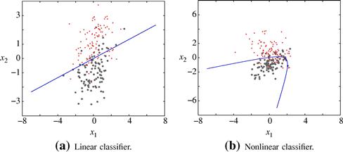
lies; typically ![]() , that is, the sign function. Figure 17.2a shows examples of two classifiers. In Figure 17.2 the classifier is linear, i.e.,
, that is, the sign function. Figure 17.2a shows examples of two classifiers. In Figure 17.2 the classifier is linear, i.e.,
![]()
and in Figure 17.2b is a nonlinear one
![]()
where

Note that, as it is apparent from both examples, the classes cannot, in general, be completely separated by the classifiers and errors in predicting the class labels are unavoidable. Tasks with separable classes are possible to occur, yet this is rather the exception than the rule.
Regression and Classification are two typical Machine Learning tasks, and a wide range of learning applications can be formulated as either one of the two. Moreover, we discussed that both tasks can be cast as parameter estimations problems, which comprise the focus of the current paper. Needless to say that both problems can also be attacked via alternative paths. For example, the k-nearest neighbor method is another possibility, which does not involve any parameter estimation phase; the only involved parameter, k, is determined via cross validation, e.g., [2].
Let us now put our parameter estimation task in a more formal setting. We are given a set of training points ![]() . For classification tasks, we replace
. For classification tasks, we replace ![]() with D. We adopt a parametric class of functions,
with D. We adopt a parametric class of functions,
![]() (17.6)
(17.6)
Our goal is to find a function in ![]() , denoted as
, denoted as ![]() , such that, given a measured value of
, such that, given a measured value of ![]() and an adopted prediction model (e.g., (17.4) for regression or (17.5) for classification), it approximates the respective output value,
and an adopted prediction model (e.g., (17.4) for regression or (17.5) for classification), it approximates the respective output value, ![]() , in an optimal way. Obviously, the word optimal paves the way to look for an optimizing criterion. To this end, a loss function is selected, from an available palette of non-negative functions,
, in an optimal way. Obviously, the word optimal paves the way to look for an optimizing criterion. To this end, a loss function is selected, from an available palette of non-negative functions,
![]() (17.7)
(17.7)
and compute ![]() so that to minimize the total loss over all the training data points, i.e.,
so that to minimize the total loss over all the training data points, i.e.,
![]() (17.8)
(17.8)
where
 (17.9)
assuming that a minimum exists. In an adaptive setting, minimizing the cost function takes place iteratively in the form
![]() (17.10)
(17.10)
as n increases. Different class of functions ![]() and different loss functions result in different estimators. In practice, for fixed number of training points, one uses cross validation to determine the “best” choice. Of course, in practice, when adaptive techniques are used and n is left to vary, cross validation techniques loose their meaning, especially when the statistical properties of the environment are slowly time varying. In such cases, the choice of the class of functions as well as the loss functions, which now has to be minimized adaptively, are empirically chosen. The critical factors, as we will see, for such choices are (a) computational complexity, (b) convergence speed, (c) tracking agility, (d) robustness to noise and to numerical error accumulation. In this paper, a number of different class functions as well as loss functions will be considered and discussed.
and different loss functions result in different estimators. In practice, for fixed number of training points, one uses cross validation to determine the “best” choice. Of course, in practice, when adaptive techniques are used and n is left to vary, cross validation techniques loose their meaning, especially when the statistical properties of the environment are slowly time varying. In such cases, the choice of the class of functions as well as the loss functions, which now has to be minimized adaptively, are empirically chosen. The critical factors, as we will see, for such choices are (a) computational complexity, (b) convergence speed, (c) tracking agility, (d) robustness to noise and to numerical error accumulation. In this paper, a number of different class functions as well as loss functions will be considered and discussed.
1.17.3 Overfitting and regularization
A problem of major importance in any Machine Learning task is that of overfitting. This is related to the complexity of the adopted model. If the model is too complex, with respect to the number of training points, N, then is tends to learn too much from the specific training set on which it is trained. For example, in regression, it tries to learn not only the useful information associated with the input data but also the contribution of the noise. So, if the model is too complex, it tends to fit very well the data points of the training set, but it does not cope well with data outside the training set; as we say, it cannot generalize well. In classification, the source of overfitting lies in the class overlap. A complex classifier will attempt to classify correctly all the points of the training set, and this is quite common in practice when very complex classifiers are employed. However, most of the class discriminatory information lies in the points lying in the “non-overlapping” regions. This is the information that a classifier has to learn in order to be able to generalize well, when faced with data outside the training set. A classifier which is designed to give very low error rates on the training set, usually results in large errors when faced with unseen data.
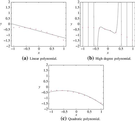
On the other hand, if our model is too simple it does not have the ability to learn even the useful information, which is contributed by the input data themselves, hence leading to very poor predictions. In practice, one seeks for a tradeoff, see, e.g., [2]. Figure 17.3 shows three cases of fitting by a very simple, a very complex and the correct model (that corresponds to the model which generated the data points). The first one is a linear model, the second one corresponds to a polynomial of high degree, i.e., 80, and the third one to a quadratic polynomial. Note that for the case of Figure 17.3b, the resulting curve passes through all the points. However, this is not what we want, since the points we have are the result of a noisy process, and the curve “follows” a path which is the combined result of the useful as well as the noise-contributed information. In practice, the performance of the resulting estimator is measured as the misfit, using a loss criterion (e.g., mean squared error, probability of error) between the predicted values and the true ones, over an independent set of data or using cross-validation techniques; for example, the resulting misfit is expected to be larger for the case of fitting the high order polynomial compared to the one corresponding to the quadratic polynomial of Figure 17.3c.
The reader may have noticed that we have avoided to define the term “complex” and we used it in a rather vague context. Complexity is often directly related to the number of the unknown parameters. However, this is not always the case. Complexity is a more general property and sometimes we may have classifiers in, even, infinite dimensional spaces, trained with a finite number of points, which generalize very well, [7].
A way to cope with the overfitting problem is to employ the regularization method. This is an elegant mathematical tool, that simultaneously cares to serve both desires; to keep the contribution of the loss function term as small as possible, since this accounts for the accuracy of the estimator, but at the same time to retain the fitted model as less complex as possible. This is achieved by adding a second term in the cost function in (17.9), whose goal is to keep the norm of the parameters as small as possible, i.e.,
 (17.11)
where ![]() is a strictly increasing monotonic non-negative function and
is a strictly increasing monotonic non-negative function and ![]() is a norm, e.g., the Euclidean
is a norm, e.g., the Euclidean ![]() or the
or the ![]() norms. The parameter
norms. The parameter ![]() is known as the regularization parameter and it controls the relative significance of the two terms in the cost function. For fixed
is known as the regularization parameter and it controls the relative significance of the two terms in the cost function. For fixed ![]() is usually determined via cross-validation. In a time varying adaptive mode of operation, when cross-validation is not possible, then empirical experience comes to assist or some adhoc techniques can be mobilized, to make
is usually determined via cross-validation. In a time varying adaptive mode of operation, when cross-validation is not possible, then empirical experience comes to assist or some adhoc techniques can be mobilized, to make ![]() , i.e., time varying. Take as an example the case where the environment does not change and the only reason that we use an adaptive algorithm is due to complexity reasons. Then, as
, i.e., time varying. Take as an example the case where the environment does not change and the only reason that we use an adaptive algorithm is due to complexity reasons. Then, as ![]() , the value of
, the value of ![]() should go to zero. For very large values of N, overfitting is no problem, since the complexity remains a small portion of the data and only the loss-related term in the cost function is sufficient. As a matter of fact, the regularization term, in this case, will only do harm by biasing the solution away from the optimum, this time without reason.
should go to zero. For very large values of N, overfitting is no problem, since the complexity remains a small portion of the data and only the loss-related term in the cost function is sufficient. As a matter of fact, the regularization term, in this case, will only do harm by biasing the solution away from the optimum, this time without reason.
Very often, ![]() is chosen so that
is chosen so that
the latter being the ![]() norm, which has been popularized in the context of sparsity-aware learning/compressed sensing. Note that, usually, the bias term is not included in the norm, since it can make the solution sensitive to the shifts of the origin. This can easily be checked out for the case of the Least Squares loss function
norm, which has been popularized in the context of sparsity-aware learning/compressed sensing. Note that, usually, the bias term is not included in the norm, since it can make the solution sensitive to the shifts of the origin. This can easily be checked out for the case of the Least Squares loss function
![]()
In practice, very often, if the mean values are not zero, we use centered data by subtracting from ![]() its sample mean, and then we can neglect
its sample mean, and then we can neglect ![]() . Besides the norm, other functions have also been used as regularizers, e.g., [8].
. Besides the norm, other functions have also been used as regularizers, e.g., [8].
Using (17.2) and plugging it in the loss function-related term (17.11), then after minimization and due to the presence of the norm-related term, some of the components of ![]() are pushed towards zero. This pushing towards zero is more aggressive when the
are pushed towards zero. This pushing towards zero is more aggressive when the ![]() norm is used, see, e.g., [9]. Obviously, the terms which are pushed to zero are those whose elimination affects the least the loss function term, which implicitly results in less complex models.
norm is used, see, e.g., [9]. Obviously, the terms which are pushed to zero are those whose elimination affects the least the loss function term, which implicitly results in less complex models.
Sparsification is another term used to indicate that the adopted estimation method has the ability to push the least significant, from the accuracy point of view (as this is measured my the loss function-related term in the regularized cost function) to zero. This is a way to guard against overfitting. Regularization techniques gain in importance and become unavoidable within a certain class of nonlinear modeling.
Consider the following modeling,
![]() (17.12)
(17.12)
![]() (17.13)
(17.13)
which, dressed with some properties, as we will soon see, is known as kernel. In other words, the expansion of our nonlinear function in (17.2) involves as many terms as our training data points, and each term in the expansion is related with one point from the training set, that is,
 (17.14)
Such models are met in the context of Support Vector Machines as well as in Relevance Vector Machines, [1,2,7]. As we will soon see, this class of models has a strong theoretical justification. In any case, such models demand drastic sparsification, otherwise they will suffer for strong overfitting. Moreover, besides overfitting, in the adaptive case, where N keeps increasing, such a model would soon become unmanageable. This paper will discuss a number of related sparsification techniques.
1.17.4 Mapping a nonlinear to a linear task
Let us now look at the expansion in (17.2) in conjunction with our prediction models given in (17.4) for the regression and (17.5) for the classification tasks. Basically, all that such a modeling says is that if we map our original input l-dimensional space into a new K-dimensional space,
![]() (17.15)
(17.15)
we expect our task to be sufficiently well modeled by adopting a linear model in this new space. It is only up to us to choose the proper functions, ![]() , as well as the appropriate dimensionality of the new space, K. For the classification task, such a procedure has a strong theoretical support from Cover’s theorem, which states that: Consider N randomly located points in an l-dimensional space and use a mapping to map these points into a higher dimensional space. Then the probability of locating them, in the new space, in linearly separable groupings tends to one as the dimensionality, K, of the new space tends to infinity. Figure 17.4 illustrates how an appropriate mapping can transform a nonlinearly separable task to a linearly separable one. Notice that nature cannot be fooled. After the mapping in the higher 2-dimensional space, the points continue to live in an l-dimensional manifold [10] (paraboloid in this case). The mapping gives the opportunity to our l-dimensional points to take advantage of the freedom, which a higher dimensional space provides, so that to move around and be placed in linearly separable positions, while retaining their original l-dimensional (true degrees of freedom) nature; a paraboloid in the 2-dimensional space can be fully described in terms of one free parameter.
, as well as the appropriate dimensionality of the new space, K. For the classification task, such a procedure has a strong theoretical support from Cover’s theorem, which states that: Consider N randomly located points in an l-dimensional space and use a mapping to map these points into a higher dimensional space. Then the probability of locating them, in the new space, in linearly separable groupings tends to one as the dimensionality, K, of the new space tends to infinity. Figure 17.4 illustrates how an appropriate mapping can transform a nonlinearly separable task to a linearly separable one. Notice that nature cannot be fooled. After the mapping in the higher 2-dimensional space, the points continue to live in an l-dimensional manifold [10] (paraboloid in this case). The mapping gives the opportunity to our l-dimensional points to take advantage of the freedom, which a higher dimensional space provides, so that to move around and be placed in linearly separable positions, while retaining their original l-dimensional (true degrees of freedom) nature; a paraboloid in the 2-dimensional space can be fully described in terms of one free parameter.

Figure 17.4 Transforming linearly non-separable learning tasks to separable ones by using nonlinear mappings to higher dimensional spaces. The original data, i.e., two “squares” and a “circle,” are placed on the 1-dimensional space, ![]() , rendering thus the linear classification task intractable. However, by using the polynomial function
, rendering thus the linear classification task intractable. However, by using the polynomial function ![]() , we are able to map the original data to a manifold which lies in the 2-dimensional space
, we are able to map the original data to a manifold which lies in the 2-dimensional space ![]() . The mapped data can be now easily linearly separated, as this can be readily verified by the linear classifier which is illustrated by the straight, black, solid line of the figure.
. The mapped data can be now easily linearly separated, as this can be readily verified by the linear classifier which is illustrated by the straight, black, solid line of the figure.
Although such a method sounds great, it has its practical drawbacks. To transform a problem into a linear one, we may have to map the original space to a very high dimensional one, and this can lead to a huge number of unknown parameters to be estimated. However, the mathematicians have, once more, offered to us an escape route that has been developed many years ago. The magic name is Reproducing Kernel Hilbert Spaces. Choosing to map to such spaces, and some of them can even be of infinite dimension, makes computations much easier; moreover, there is an associated strong theorem that justifies the expansion in (17.14). Assume that we have selected a mapping
![]() (17.16)
(17.16)
where ![]() is RKHS. Then, the following statements are valid:
is RKHS. Then, the following statements are valid:
• The Kernel Trick: Let ![]() be two points in our original l-dimensional space and
be two points in our original l-dimensional space and ![]() their respective images in an RKHS,
their respective images in an RKHS, ![]() . Since
. Since ![]() is a Hilbert space, an inner product,
is a Hilbert space, an inner product, ![]() , is associated with it, by the definition of Hilbert spaces. As we will more formally see in the next section, the inner product of any RKHS is uniquely defined in terms of the so called kernel function,
, is associated with it, by the definition of Hilbert spaces. As we will more formally see in the next section, the inner product of any RKHS is uniquely defined in terms of the so called kernel function, ![]() and the following holds true
and the following holds true
![]() (17.17)
(17.17)
This is a remarkable property, since it allows to compute inner products in a (high dimensional) RKHS as a function operating in the lower dimensional input space. Also, this property allows the following “black box” approach, that has extensively been exploited in Machine Learning:
– Design an algorithm, which operates in the input space and computes the estimates of the parameters of a linear modeling.
– Cast this algorithm, if of course this is possible, in terms of inner product operations only.
– Replace each inner product with a kernel operation.
Then the resulting algorithm is equivalent with solving the (linear modeling) estimation task in an RKHS, which is defined by the selected kernel. Different kernel functions correspond to different RKHSs and, consequently, to different nonlinearities; each inner product in the RKHS is a nonlinear function operation in the input space. The kernel trick was first used in [11,12].
• Representer Theorem: Consider the cost function in (17.11), and constrain the solutions to lie within an RKHS space, defined by a kernel function ![]() . Then the minimizer of (17.11) is of the form
. Then the minimizer of (17.11) is of the form
 (17.18)
This makes crystal clear the reason for the specific modeling in (17.14). In other words, if we choose to attack a nonlinear modeling by “transforming” it to a linear one, after performing a mapping of our data into a RKHS in order to exploit the advantage of efficient inner product operations, then the (linear with respect to the parameters) modeling in (17.14) results naturally from the theory. Our only concern now is to use an appropriate regularization, in order to cope with overfitting problems.
All the previously presented issues will be discussed in more detail in the sections to come. Our goal, so far, was to try to give the big picture of the paper in simple terms and focus more on the notions than on mathematics. We will become more formal in the sections to come. The reader, however, may bypass some of the sections, if his/her current focus is not on the mathematical details but on the algorithms. As said already before, we have made an effort to write the paper in such a way, so that to serve both needs: mathematical rigor and practical flavor, as much as we could.
1.17.5 Reproducing Kernel Hilbert spaces
In kernel-based methods, the notion of the Reproducing Kernel Hilbert Space (RKHS) plays a crucial role. A RKHS is a rich construct (roughly, a space of functions with an inner product), which has been proven to be a very powerful tool. Kernel-based methods are utilized in an increasingly large number of scientific areas, especially where nonlinear models are required. For example, in pattern analysis, a classification task of a set ![]() is usually reformed by mapping the data into a higher dimensional space (possibly of infinite dimension)
is usually reformed by mapping the data into a higher dimensional space (possibly of infinite dimension) ![]() , which is a Reproducing Kernel Hilbert Space (RKHS). The advantage of such a mapping is to make the task more tractable, by employing a linear classifier in the feature space
, which is a Reproducing Kernel Hilbert Space (RKHS). The advantage of such a mapping is to make the task more tractable, by employing a linear classifier in the feature space ![]() , exploiting Cover’s theorem (see [2,13]). This is equivalent with solving a nonlinear problem in the original space.
, exploiting Cover’s theorem (see [2,13]). This is equivalent with solving a nonlinear problem in the original space.
Similar approaches have been used in principal components analysis, in Fisher’s linear discriminant analysis, in clustering, regression, image processing and in many other subdisciplines. Recently, processing in RKHS is gaining in popularity within the Signal Processing community in the context of adaptive learning.
Although the kernel trick works well for most applications, it may conceal the basic mathematical steps that underlie the procedure, which are essential if one seeks a deeper understanding of the problem. These steps are: 1) Map the finite dimensionality input data from the input space X (usually ![]() ) into a higher dimensionality (possibly infinite) RKHS
) into a higher dimensionality (possibly infinite) RKHS ![]() (feature space) and 2) Perform a linear processing (e.g., adaptive filtering) on the mapped data in
(feature space) and 2) Perform a linear processing (e.g., adaptive filtering) on the mapped data in ![]() . The procedure is equivalent with a nonlinear processing (nonlinear filtering) in X (see Figure 17.5). The specific choice of the kernel
. The procedure is equivalent with a nonlinear processing (nonlinear filtering) in X (see Figure 17.5). The specific choice of the kernel ![]() defines, implicitly, an RKHS with an appropriate inner product. Moreover, the specific choice of the kernel defines the type of nonlinearity that underlies the model to be used.
defines, implicitly, an RKHS with an appropriate inner product. Moreover, the specific choice of the kernel defines the type of nonlinearity that underlies the model to be used.

1.17.5.1 A historical overview
In the past, there have been two trends in the study of these spaces by the mathematicians. The first one originated in the theory of integral equations by Mercer [14,15]. He used the term “positive definite kernel” to characterize a function of two points ![]() defined on
defined on ![]() , which satisfies Mercer’s theorem:
, which satisfies Mercer’s theorem:
 (17.19)
for any numbers ![]() , any points
, any points ![]() ,
, ![]() , and for all
, and for all ![]() . Later on, Moore [16–18] found that to such a kernel there corresponds a well determined class of functions,
. Later on, Moore [16–18] found that to such a kernel there corresponds a well determined class of functions, ![]() , equipped with a specific inner product
, equipped with a specific inner product ![]() , in respect to which the kernel
, in respect to which the kernel ![]() possesses the so called reproducing property:
possesses the so called reproducing property:
![]() (17.20)
(17.20)
for all functions ![]() and
and ![]() . Those that followed this trend used to consider a specific given positive definite kernel
. Those that followed this trend used to consider a specific given positive definite kernel ![]() and studied it in itself, or eventually applied it in various domains (such as integral equations, theory of groups, general metric theory, interpolation, etc.). The class
and studied it in itself, or eventually applied it in various domains (such as integral equations, theory of groups, general metric theory, interpolation, etc.). The class ![]() corresponding to
corresponding to ![]() was mainly used as a tool of research and it was usually introduced a posteriori. The work of Bochner [19,20], which introduced the notion of the “positive definite function” in order to apply it in the theory of Fourier transforms, also belongs to the same path as the one followed by Mercer and Moore.
was mainly used as a tool of research and it was usually introduced a posteriori. The work of Bochner [19,20], which introduced the notion of the “positive definite function” in order to apply it in the theory of Fourier transforms, also belongs to the same path as the one followed by Mercer and Moore.
On the other hand, those who followed the second trend were primarily interested in the class of functions ![]() , while the associated kernel was employed essentially as a tool in the study of the functions of this class. This trend is traced back to the works of Zaremba [21,22] during the first decade of the 20th century. He was the first to introduce the notion of a kernel, which corresponds to a specific class of functions and to state its reproducing property. However, he did not develop any general theory, nor did he gave any particular name to the kernels he introduced. In this, second trend, the mathematicians were primarily interested in the study of the class of functions
, while the associated kernel was employed essentially as a tool in the study of the functions of this class. This trend is traced back to the works of Zaremba [21,22] during the first decade of the 20th century. He was the first to introduce the notion of a kernel, which corresponds to a specific class of functions and to state its reproducing property. However, he did not develop any general theory, nor did he gave any particular name to the kernels he introduced. In this, second trend, the mathematicians were primarily interested in the study of the class of functions ![]() and the corresponding kernel
and the corresponding kernel ![]() , which satisfies the reproducing property, was used as a tool in this study. To the same trend belong also the works of Bergman [23] and Aronszajn [3]. Those two trends evolved separately during the first decades of the 20th century, but soon the links between them were noticed. After the second world war, it was known that the two concepts of defining a kernel, either as a positive definite kernel, or as a reproducing kernel, are equivalent. Furthermore, it was proved that there is a one to one correspondence between the space of positive definite kernels and the space of reproducing kernel Hilbert spaces.
, which satisfies the reproducing property, was used as a tool in this study. To the same trend belong also the works of Bergman [23] and Aronszajn [3]. Those two trends evolved separately during the first decades of the 20th century, but soon the links between them were noticed. After the second world war, it was known that the two concepts of defining a kernel, either as a positive definite kernel, or as a reproducing kernel, are equivalent. Furthermore, it was proved that there is a one to one correspondence between the space of positive definite kernels and the space of reproducing kernel Hilbert spaces.
It has to be emphasized that examples of such kernels have been known for a long time prior to the works of Mercer and Zaremba; for example, all the Green’s functions of self-adjoint ordinary differential equations belong to this type of kernels. However, some of the important properties that these kernels possess have only been realized and used in the beginning of the 20th century and since then have been the focus of research. In the following, we will give a more detailed description of these spaces and establish their main properties, focusing on the essentials that elevate them to such a powerful tool in the context of machine learning. Most of the material presented here can also be found in more detail in several other papers and textbooks, such as the celebrated paper of Aronszajn [3], the excellent introductory text of Paulsen [24] and the popular books of Schölkoph and Smola [13] and Shawe-Taylor and Cristianini [25]. Here, we attempt to portray both trends and to highlight the important links between them. Although the general theory applies to complex spaces, to keep the presentation as simple as possible, we will mainly focus on real spaces.
1.17.5.2 Definition
We begin our study with the classic definitions on positive definite matrices and kernels as they were introduced by Mercer. Given a function ![]() and
and ![]() (typically X is a compact subset of
(typically X is a compact subset of ![]() ), the square matrix
), the square matrix ![]() with elements
with elements ![]() , for
, for ![]() , is called the Gram matrix (or kernel matrix) of
, is called the Gram matrix (or kernel matrix) of ![]() with respect to
with respect to ![]() . A symmetric matrix
. A symmetric matrix ![]() satisfying
satisfying

for all ![]() ,
, ![]() , where the notation
, where the notation ![]() denotes transposition, is called positive definite. In matrix analysis literature, this is the definition of a positive semidefinite matrix. However, as positive definite matrices were originally introduced by Mercer and others in this context, we employ the term positive definite, as it was already defined. If the inequality is strict, for all non-zero vectors
denotes transposition, is called positive definite. In matrix analysis literature, this is the definition of a positive semidefinite matrix. However, as positive definite matrices were originally introduced by Mercer and others in this context, we employ the term positive definite, as it was already defined. If the inequality is strict, for all non-zero vectors ![]() , the matrix will be called strictly positive definite. A function
, the matrix will be called strictly positive definite. A function ![]() , which for all
, which for all ![]() and all
and all ![]() gives rise to a positive definite Gram matrix K, is called a positive definite kernel. In the following, we will frequently refer to a positive definite kernel simply as kernel. We conclude that a positive definite kernel is symmetric and satisfies
gives rise to a positive definite Gram matrix K, is called a positive definite kernel. In the following, we will frequently refer to a positive definite kernel simply as kernel. We conclude that a positive definite kernel is symmetric and satisfies

for all ![]() ,
, ![]() , and for all
, and for all ![]() . Formally, a Reproducing Kernel Hilbert space is defined as follows:
. Formally, a Reproducing Kernel Hilbert space is defined as follows:
Definition 1
Reproducing Kernel Hilbert Space (RKHS)
Consider a linear space ![]() of real valued functions, f, defined on a set X. Suppose, further, that in
of real valued functions, f, defined on a set X. Suppose, further, that in ![]() we can define an inner product
we can define an inner product ![]() with corresponding norm
with corresponding norm ![]() and that
and that ![]() is complete with respect to that norm, i.e.,
is complete with respect to that norm, i.e., ![]() is a Hilbert space. We call
is a Hilbert space. We call ![]() a Reproducing Kernel Hilbert Space (RKHS), if there exists a function
a Reproducing Kernel Hilbert Space (RKHS), if there exists a function ![]() with the following two important properties:
with the following two important properties:
1. For every ![]() belongs to
belongs to ![]() (or equivalently
(or equivalently ![]() spans
spans ![]() , i.e.,
, i.e., ![]() , where the overline stands for the closure of a set).
, where the overline stands for the closure of a set).
2. ![]() has the so called reproducing property, i.e.,
has the so called reproducing property, i.e.,
![]() (17.21)
(17.21)
in particular ![]() . Furthermore,
. Furthermore, ![]() is a positive definite kernel and the mapping
is a positive definite kernel and the mapping ![]() , with
, with ![]() , for all
, for all ![]() is called the feature map of
is called the feature map of ![]() .
.
![]()
To denote the RKHS associated with a specific kernel ![]() , we will also use the notation
, we will also use the notation ![]() . Furthermore, under the aforementioned notations
. Furthermore, under the aforementioned notations ![]() , i.e.,
, i.e., ![]() is the inner product of
is the inner product of ![]() and
and ![]() in the feature space. This is the essence of the kernel trick mentioned in Section 1.17.4. The feature map
in the feature space. This is the essence of the kernel trick mentioned in Section 1.17.4. The feature map ![]() transforms the data from the low dimensionality space X to the higher dimensionality feature space
transforms the data from the low dimensionality space X to the higher dimensionality feature space ![]() . Linear processing in
. Linear processing in ![]() involves inner products in
involves inner products in ![]() , which can be calculated via the kernel
, which can be calculated via the kernel ![]() disregarding the actual structure of
disregarding the actual structure of ![]() .
.
1.17.5.3 Some basic theorems
In the following, we consider the definition of a RKHS as a class of functions with specific properties (following the second trend) and show the key ideas that underlie Definition 1. To that end, consider a linear class ![]() of real valued functions, f, defined on a set X. Suppose, further, that in
of real valued functions, f, defined on a set X. Suppose, further, that in ![]() we can define an inner product
we can define an inner product ![]() with corresponding norm
with corresponding norm ![]() and that
and that ![]() is complete with respect to that norm, i.e.,
is complete with respect to that norm, i.e., ![]() is a Hilbert space. Consider, also, a linear functional T, from
is a Hilbert space. Consider, also, a linear functional T, from ![]() into the field
into the field ![]() . An important theorem of functional analysis states that such a functional is continuous, if and only if it is bounded. The space consisting of all continuous linear functionals from
. An important theorem of functional analysis states that such a functional is continuous, if and only if it is bounded. The space consisting of all continuous linear functionals from ![]() into the field
into the field ![]() is called the dual space of
is called the dual space of ![]() . In the following, we will frequently refer to the so called linear evaluation functional
. In the following, we will frequently refer to the so called linear evaluation functional ![]() . This is a special case of a linear functional that satisfies
. This is a special case of a linear functional that satisfies ![]() , for all
, for all ![]() .
.
We call ![]() a Reproducing Kernel Hilbert Space (RKHS) on X over
a Reproducing Kernel Hilbert Space (RKHS) on X over ![]() , if for every
, if for every ![]() , the linear evaluation functional,
, the linear evaluation functional, ![]() , is continuous. We will prove that such a space is related to a positive definite kernel, thus providing the first link between the two trends. Subsequently, we will prove that any positive definite kernel defines implicitly a RKHS, providing the second link and concluding the equivalent definition of RKHS (Definition 1), which is usually used in the machine learning literature. The following theorem establishes an important connection between a Hilbert space H and its dual space.
, is continuous. We will prove that such a space is related to a positive definite kernel, thus providing the first link between the two trends. Subsequently, we will prove that any positive definite kernel defines implicitly a RKHS, providing the second link and concluding the equivalent definition of RKHS (Definition 1), which is usually used in the machine learning literature. The following theorem establishes an important connection between a Hilbert space H and its dual space.
Theorem 2
Riesz Representation
Let ![]() be a general Hilbert space and let
be a general Hilbert space and let ![]() denote its dual space. Every element
denote its dual space. Every element ![]() of
of ![]() can be uniquely expressed in the form:
can be uniquely expressed in the form:
![]()
for some ![]() . Moreover,
. Moreover, ![]() .
. ![]()
Following the Riesz representation theorem, we have that for every ![]() , there exists a unique element
, there exists a unique element ![]() , such that for every
, such that for every ![]() ,
, ![]() . The function
. The function ![]() is called the reproducing kernel for the point
is called the reproducing kernel for the point ![]() and the function
and the function ![]() is called the reproducing kernel of
is called the reproducing kernel of ![]() . In addition, note that
. In addition, note that ![]() and
and ![]() .
.
Proposition 3
The reproducing kernel of ![]() is symmetric, i.e.,
is symmetric, i.e., ![]() .
. ![]()
Proof
Observe that ![]() and
and ![]() . As the inner product of
. As the inner product of ![]() is symmetric (i.e.,
is symmetric (i.e., ![]() ) the result follows.
) the result follows. ![]()
In the following, we will frequently identify the function ![]() with the notation
with the notation ![]() . Thus, we write the reproducing property of
. Thus, we write the reproducing property of ![]() as:
as:
![]() (17.22)
(17.22)
for any ![]() ,
, ![]() . Note that due to the uniqueness provided by the Riesz representation theorem,
. Note that due to the uniqueness provided by the Riesz representation theorem, ![]() is the unique function that satisfies the reproducing property. The following proposition establishes the first link between the positive definite kernels and the reproducing kernels.
is the unique function that satisfies the reproducing property. The following proposition establishes the first link between the positive definite kernels and the reproducing kernels.
Proposition 4
The reproducing kernel of ![]() is a positive definite kernel.
is a positive definite kernel. ![]()
Proof
Consider ![]() , the real numbers
, the real numbers ![]() and the elements,
and the elements, ![]() . Then
. Then
Combining Proposition 3 and the previous result, we complete the proof. ![]()
Remark 5
In general, the respective Gram matrix associated with a reproducing kernel is strictly positive definite. For if not, then there must exist at least one non zero vector ![]() such that
such that ![]() , for some finite set of points
, for some finite set of points ![]() . Hence, for every
. Hence, for every ![]() , we have that
, we have that ![]() . Thus, in this case there exists a linear dependence between the values of every function in
. Thus, in this case there exists a linear dependence between the values of every function in ![]() at some finite set of points. Such examples do exist (e.g., Sobolev spaces), but in most cases the reproducing kernels define Gram matrices that are always strictly positive and invertible.
at some finite set of points. Such examples do exist (e.g., Sobolev spaces), but in most cases the reproducing kernels define Gram matrices that are always strictly positive and invertible.
The following proposition establishes a very important fact; any RKHS, ![]() , can be generated by the respective reproducing kernel
, can be generated by the respective reproducing kernel ![]() . Note that the overline denotes the closure of a set (i.e., if A is a subset of
. Note that the overline denotes the closure of a set (i.e., if A is a subset of ![]() is the closure of A).
is the closure of A).
Proposition 6
Let ![]() be a RKHS on the set X with reproducing kernel
be a RKHS on the set X with reproducing kernel ![]() . Then the linear span of the functions
. Then the linear span of the functions ![]() ,
, ![]() , is dense in
, is dense in ![]() , i.e.,
, i.e., ![]() .
. ![]()
Proof
We will prove that the only function of ![]() orthogonal to
orthogonal to ![]() is the zero function. Let f be such a function. Then, as f is orthogonal to A, we have that
is the zero function. Let f be such a function. Then, as f is orthogonal to A, we have that ![]() , for every
, for every ![]() . This holds true if and only if
. This holds true if and only if ![]() . Thus
. Thus ![]() . Suppose that there is
. Suppose that there is ![]() such that
such that ![]() . As
. As ![]() is a closed (convex) subspace of
is a closed (convex) subspace of ![]() , there is a
, there is a ![]() which minimizes the distance between f and points in
which minimizes the distance between f and points in ![]() (theorem of best approximation). For the same g we have that
(theorem of best approximation). For the same g we have that ![]() . Thus, the non-zero function
. Thus, the non-zero function ![]() is orthogonal to
is orthogonal to ![]() . However, we proved that there isn’t any non-zero vector orthogonal to A. This leads us to conclude that
. However, we proved that there isn’t any non-zero vector orthogonal to A. This leads us to conclude that ![]() .
. ![]()
In the following we give some important properties of the specific spaces.
Proposition 7
Norm convergence implies point-wise convergence
Let ![]() be a RKHS on X and let
be a RKHS on X and let ![]() . If
. If ![]() , then
, then ![]() , for every
, for every ![]() . Conversely, if for any sequence
. Conversely, if for any sequence ![]() of a Hilbert space
of a Hilbert space ![]() , such that
, such that ![]() , we have also that
, we have also that ![]() , then
, then ![]() is a RKHS.
is a RKHS. ![]()
Proof
For every ![]() we have that
we have that
![]()
As ![]() , we have that
, we have that ![]() , for every
, for every ![]() . Hence
. Hence ![]() , for every
, for every ![]() .
.
For the converse, consider the evaluation functional ![]() for some
for some ![]() . We will prove that
. We will prove that ![]() is continuous for all
is continuous for all ![]() . To this end, consider a sequence
. To this end, consider a sequence ![]() of
of ![]() , with the property
, with the property ![]() , i.e.,
, i.e., ![]() converges to f in the norm. Then
converges to f in the norm. Then ![]() , as
, as ![]() . Thus
. Thus ![]() for all
for all ![]() and all converging sequences
and all converging sequences ![]() of
of ![]() .
. ![]()
Proposition 8
Different RKHS’s cannot have the same reproducing kernel
Let ![]() be RKHS’s on X with reproducing kernels
be RKHS’s on X with reproducing kernels ![]() . If
. If ![]() , for all
, for all ![]() , then
, then ![]() and
and ![]() for every f.
for every f. ![]()
Proof
Let ![]() and
and ![]() . As shown in Proposition 6,
. As shown in Proposition 6, ![]() . Note that for any
. Note that for any ![]() , we have that
, we have that ![]() , for some real numbers
, for some real numbers ![]() and thus the values of the function are independent of whether we regard it as in
and thus the values of the function are independent of whether we regard it as in ![]() or
or ![]() . Furthermore, for any
. Furthermore, for any ![]() , as the two kernels are identical, we have that
, as the two kernels are identical, we have that ![]() . Thus,
. Thus, ![]() , for all
, for all ![]() .
.
Finally, we turn our attention to the limit points of ![]() and
and ![]() . If
. If ![]() , then there exists a sequence of functions,
, then there exists a sequence of functions, ![]() such that
such that ![]() . Since
. Since ![]() is a converging sequence, it is Cauchy in
is a converging sequence, it is Cauchy in ![]() and thus it is also Cauchy in
and thus it is also Cauchy in ![]() . Therefore, there exists
. Therefore, there exists ![]() such that
such that ![]() . Employing proposition 7, we take that
. Employing proposition 7, we take that ![]() . Thus, every f in
. Thus, every f in ![]() is also in
is also in ![]() and by analogous argument we can prove that every
and by analogous argument we can prove that every ![]() is also in
is also in ![]() . Hence,
. Hence, ![]() and as
and as ![]() for all f in a dense subset (i.e.,
for all f in a dense subset (i.e., ![]() ), we have that the norms are equal for every f. To prove the latter, we use the relation
), we have that the norms are equal for every f. To prove the latter, we use the relation ![]() .
. ![]()
The following theorem is the converse of Proposition 4. It was proved by Moore and it gives us a characterization of reproducing kernel functions. Also, it provides the second link between the two trends that have been mentioned in Section 1.17.5.1. Moore’s theorem, together with Proposition 4, Proposition 8 and the uniqueness property of the reproducing kernel of a RKHS, establishes a one-to-one correspondence between RKHS’s on a set and positive definite functions on the set.
Theorem 9
Moore [16]
Let X be a set and let ![]() be a positive definite kernel. Then there exists a RKHS of functions on X, such that
be a positive definite kernel. Then there exists a RKHS of functions on X, such that ![]() is the reproducing kernel of
is the reproducing kernel of ![]() .
. ![]()
Proof
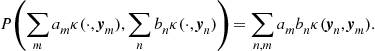
We will give only a sketch of the proof. The interested reader is referred to [24]. The first step is to define ![]() and the linear map
and the linear map ![]() such that
such that
We prove that P is well defined and that it satisfies the properties of the inner product. Then, given the vector space A and the inner product P, one may complete the space by taking equivalence classes of Cauchy sequences from A to obtain the Hilbert space ![]() . Finally, the reproducing property of the kernel
. Finally, the reproducing property of the kernel ![]() with respect to the inner product P is proved.
with respect to the inner product P is proved. ![]()
In view of the aforementioned theorems, the Definition 1 of the RKHS given in 1.17.5.2, which is usually used in the machine learning literature, follows naturally.
We conclude this section with a short description of the most important points of the theory developed by Mercer in the context of integral operators. Mercer considered integral operators ![]() generated by a kernel
generated by a kernel ![]() , i.e.,
, i.e., ![]() , such that
, such that ![]() . He concluded the following theorem [14]:
. He concluded the following theorem [14]:
Theorem 10
Mercer kernels are positive definite [14]
Let ![]() be a nonempty set and let
be a nonempty set and let ![]() be continuous. Then
be continuous. Then ![]() is a positive definite kernel, if and only if,
is a positive definite kernel, if and only if,
![]()
for all functions ![]() . Moreover, if
. Moreover, if ![]() is positive definite, the integral operator
is positive definite, the integral operator ![]() is positive definite, that is,
is positive definite, that is,
![]()
for all ![]() , and if
, and if ![]() are the normalized orthogonal eigenfunctions of
are the normalized orthogonal eigenfunctions of ![]() associated with the eigenvalues
associated with the eigenvalues ![]() then:
then:
![]()
![]()
Note that the original form of above theorem is more general, involving ![]() -algebras and probability measures. However, as in the applications concerning this manuscript such general terms are of no importance, we decided to include this simpler form. The previous theorems established that Mercer’s kernels, as they are positive definite kernels, are also reproducing kernels. Furthermore, the first part of Theorem 10 provides a useful tool of determining whether a specific function is actually a reproducing kernel.
-algebras and probability measures. However, as in the applications concerning this manuscript such general terms are of no importance, we decided to include this simpler form. The previous theorems established that Mercer’s kernels, as they are positive definite kernels, are also reproducing kernels. Furthermore, the first part of Theorem 10 provides a useful tool of determining whether a specific function is actually a reproducing kernel.
1.17.5.4 Examples of kernels
Before proceeding to some more advanced topics in the theory of RKHS, it is important to give some examples of kernels that appear more often in the literature and are used in various applications. Perhaps the most widely used reproducing kernel is the Gaussian radial basis function defined on ![]() , where
, where ![]() , as:
, as:
 (17.23)
where ![]() . Equivalently the Gaussian RBF function can be defined as:
. Equivalently the Gaussian RBF function can be defined as:
![]() (17.24)
(17.24)
for ![]() . Other well-known kernels defined in
. Other well-known kernels defined in ![]() are:
are:
• The homogeneous polynomial kernel: ![]() .
.
• The inhomogeneous polynomial kernel: ![]() , where
, where ![]() a constant.
a constant.
Note that the RKHS associated to the Gaussian RBF kernel and the Laplacian kernel are infinite dimensional, while the RKHS associated to the polynomial kernels have finite dimension [13]. Figures 17.6–17.10, show some of the aforementioned kernels together with a sample of the elements ![]() that span the respective RKHS’s for the case
that span the respective RKHS’s for the case ![]() . Figures 17.11–17.13, show some of the elements
. Figures 17.11–17.13, show some of the elements ![]() that span the respective RKHS’s for the case
that span the respective RKHS’s for the case ![]() . Interactive figures regarding the aforementioned examples can be found in http://bouboulis.mysch.gr/kernels.html. Moreover, Appendix A highlights several properties of the popular Gaussian kernel.
. Interactive figures regarding the aforementioned examples can be found in http://bouboulis.mysch.gr/kernels.html. Moreover, Appendix A highlights several properties of the popular Gaussian kernel.
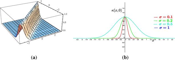
Figure 17.6 (a) The Gaussian kernel for the case ![]() ,
, ![]() . (b) The element
. (b) The element ![]() of the feature space induced by the Gaussian kernel for various values of the parameter
of the feature space induced by the Gaussian kernel for various values of the parameter ![]() .
.
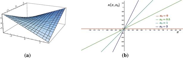
Figure 17.7 (a) The homogeneous polynomial kernel for the case ![]() ,
, ![]() . (b) The element
. (b) The element ![]() ,
, ![]() of the feature space induced by the homogeneous polynomial kernel
of the feature space induced by the homogeneous polynomial kernel ![]() for various values of
for various values of ![]() .
.

Figure 17.8 (a) The homogeneous polynomial kernel for the case ![]() ,
, ![]() . (b) The element
. (b) The element ![]() ,
, ![]() of the feature space induced by the homogeneous polynomial kernel
of the feature space induced by the homogeneous polynomial kernel ![]() for various values of
for various values of ![]() .
.

Figure 17.9 (a) The inhomogeneous polynomial kernel for the case ![]() ,
, ![]() . (b) The element
. (b) The element ![]() ,
, ![]() of the feature space induced by the inhomogeneous polynomial kernel
of the feature space induced by the inhomogeneous polynomial kernel ![]() for various values of
for various values of ![]() .
.
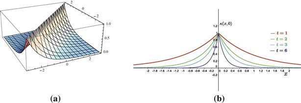
Figure 17.10 (a) The Laplacian kernel for the case ![]() ,
, ![]() . (b) The element
. (b) The element ![]() of the feature space induced by the Laplacian kernel for various values of the parameter t.
of the feature space induced by the Laplacian kernel for various values of the parameter t.


1.17.5.5 Some properties of the RKHS
In this section, we will refer to some more advanced topics on the theory of RKHS, which are useful for a deeper understanding of the underlying theory and show why RKHS’s constitute such a powerful tool. We begin our study with some properties of RKHS’s and conclude with the basic theorems that enable us to generate new kernels. As we work in Hilbert spaces, the two Parseval’s identities are an extremely helpful tool. When ![]() (where S is an arbitrary set) is an orthonormal basis for a Hilbert space
(where S is an arbitrary set) is an orthonormal basis for a Hilbert space ![]() , then for any
, then for any ![]() we have that:
we have that:
![]() (17.25)
(17.25)
![]() (17.26)
(17.26)
Note that these two identities hold for a general arbitrary set S (not necessarily ordered). The convergence in this case is defined somewhat differently. We say that ![]() , if for any
, if for any ![]() , there exists a finite subset
, there exists a finite subset ![]() , such that for any finite set
, such that for any finite set ![]() , we have that
, we have that ![]() .
.
Proposition 11
Cauchy-Schwarz Inequality
If ![]() is a reproducing kernel on X then
is a reproducing kernel on X then
![]()
![]()
Proof
The proof is straightforward, as ![]() is the inner product
is the inner product ![]() of the space
of the space ![]() .
. ![]()
Theorem 12
Every finite dimensional class of functions defined on X, equipped with an inner product, is an RKHS. Let ![]() constitute a basis of the space and the inner product is defined as follows
constitute a basis of the space and the inner product is defined as follows

for ![]() and
and ![]() , where the
, where the ![]() real matrix
real matrix ![]() is strictly positive definite. Let
is strictly positive definite. Let ![]() be the inverse of A, then the kernel of the RKHS is given by
be the inverse of A, then the kernel of the RKHS is given by
 (17.27)
![]()

The following theorem gives the kernel of a RKHS (of finite or infinite dimension) in terms of the elements of an orthonormal basis.
Theorem 13
Let ![]() be a RKHS on X with reproducing kernel
be a RKHS on X with reproducing kernel ![]() . If
. If ![]() is an orthonormal basis for
is an orthonormal basis for ![]() , then
, then ![]() , where this series converges pointwise.
, where this series converges pointwise. ![]()
Proof
For any ![]() we have that
we have that ![]() . Hence, employing Parseval’s identity (17.25), we have that
. Hence, employing Parseval’s identity (17.25), we have that ![]() , where these sums converge in the norm on
, where these sums converge in the norm on ![]() . Since the sums converge in the norm, they converge at every point. Hence,
. Since the sums converge in the norm, they converge at every point. Hence, ![]() .
. ![]()
Proposition 14
If ![]() is a RKHS on X with respective kernel
is a RKHS on X with respective kernel ![]() , then every closed subspace
, then every closed subspace ![]() is also a RKHS. In addition, if
is also a RKHS. In addition, if ![]() and
and ![]() are complementary subspaces in
are complementary subspaces in ![]() then
then ![]() .
. ![]()
Proposition 15
Let ![]() be a RKHS on X with kernel
be a RKHS on X with kernel ![]() and
and ![]() is an orthonormal system in
is an orthonormal system in ![]() . Then for any sequence of numbers
. Then for any sequence of numbers ![]() such that
such that ![]() (i.e.,
(i.e., ![]() ) we have
) we have

Proof
We have seen that ![]() and that
and that ![]() . Thus, considering that
. Thus, considering that ![]() ’s are orthonormal and taking the Parseval’s identity (17.26) for
’s are orthonormal and taking the Parseval’s identity (17.26) for ![]() with respect to the orthonormal basis, we have:
with respect to the orthonormal basis, we have:
![]()
Therefore, applying the Cauchy-Schwartz inequality we take

Theorem 16
Representer Theorem [26]
Denote by ![]() a strictly monotonic increasing function, by X a nonempty set and by
a strictly monotonic increasing function, by X a nonempty set and by ![]() an arbitrary loss function. Then each minimizer
an arbitrary loss function. Then each minimizer ![]() of the regularized minimization problem:
of the regularized minimization problem:
![]()
admits a representation of the form
 (17.28)
where ![]() , for
, for ![]() .
. ![]()
Proof
We may decompose each ![]() into a part contained in the span of the kernels centered at the training points, i.e.,
into a part contained in the span of the kernels centered at the training points, i.e., ![]() , (which is a closed linear subspace) and a part in the orthogonal complement of the previous span. Thus each f can be written as:
, (which is a closed linear subspace) and a part in the orthogonal complement of the previous span. Thus each f can be written as:
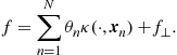
Applying the reproducing property and considering that ![]() , for
, for ![]() , we take:
, we take:

Thus, the value of the loss function ![]() depends only on the part contained in the span of the kernels centered at the training points, i.e., on
depends only on the part contained in the span of the kernels centered at the training points, i.e., on ![]() . Furthermore, for all
. Furthermore, for all ![]() we have:
we have:

Thus, for any fixed ![]() the value of the cost function is minimized for
the value of the cost function is minimized for ![]() . Hence, the solution of the minimization task will have to obey this property too.
. Hence, the solution of the minimization task will have to obey this property too. ![]()
Examples of loss functions ![]() as the ones mentioned in Theorem 16 are for example the total squared error:
as the ones mentioned in Theorem 16 are for example the total squared error:
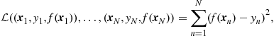
and the ![]() norm measured error
norm measured error
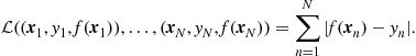
The aforementioned theorem is of great importance to practical applications. Although one might be trying to solve an optimization task in an infinite dimensional RKHS ![]() (such as the one that generated by the Gaussian kernel), the Representer Theorem states that the solution of the problem lies in the span of N particular kernels, those centered on the training points.
(such as the one that generated by the Gaussian kernel), the Representer Theorem states that the solution of the problem lies in the span of N particular kernels, those centered on the training points.
In practice, we often include a bias factor to the solution of kernel-based regularized minimization tasks, that is, we assume that f admits a representation of the form
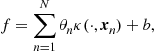 (17.29)
where ![]() . This has been shown to improve the performance of the respective algorithms [2,13,27], for two main reasons. Firstly, the introduction of the bias, b, enlarges the family of functions in which we search for a solution, thus leading to potentially better estimations. Moreover, as the regularization factor
. This has been shown to improve the performance of the respective algorithms [2,13,27], for two main reasons. Firstly, the introduction of the bias, b, enlarges the family of functions in which we search for a solution, thus leading to potentially better estimations. Moreover, as the regularization factor ![]() penalizes the values of f at the training points, the resulting solution tends to take values as close to zero as possible, for large values of
penalizes the values of f at the training points, the resulting solution tends to take values as close to zero as possible, for large values of ![]() (compare Figures 17.14b and 17.14d). At this point, another comment is of interest also. Note that it turns out that the regularization factor
(compare Figures 17.14b and 17.14d). At this point, another comment is of interest also. Note that it turns out that the regularization factor ![]() for certain types of kernel functions (e.g., Gaussian) involves the derivatives of f of all orders [13,28]. As a consequence the larger the
for certain types of kernel functions (e.g., Gaussian) involves the derivatives of f of all orders [13,28]. As a consequence the larger the ![]() is, the smoother the resulting curve becomes (compare Figures 17.14a with 17.14c and Figures 17.14b with 17.14d). The use of the bias factor is theoretically justified by the semi-parametric Representer theorem.
is, the smoother the resulting curve becomes (compare Figures 17.14a with 17.14c and Figures 17.14b with 17.14d). The use of the bias factor is theoretically justified by the semi-parametric Representer theorem.
Theorem 17
Semi-parametric Representer Theorem [13]
Suppose that in addition to the assumptions of theorem 16, we are given a set of M real valued functions ![]() , with the property that the
, with the property that the ![]() matrix
matrix ![]() has rank M. Then any
has rank M. Then any ![]() , with
, with ![]() and
and ![]() , solving
, solving
![]()
admits a representation of the form
 (17.30)
with ![]() , for all
, for all ![]() .
. ![]()

Figure 17.14 Solving the regression problem ![]() , on a set of 11 points (a), (c) with a bias, i.e., f admits the form of (17.29) and (b), (d) without a bias, i.e., f admits the form of (17.28). In all the examples the Gaussian kernel function was employed. In (a) and (b) we set
, on a set of 11 points (a), (c) with a bias, i.e., f admits the form of (17.29) and (b), (d) without a bias, i.e., f admits the form of (17.28). In all the examples the Gaussian kernel function was employed. In (a) and (b) we set ![]() ,
, ![]() . In (c) and (d) we set
. In (c) and (d) we set ![]() ,
, ![]() . Observe that for
. Observe that for ![]() , the unbiased solution takes values significantly lower compared to the values of the training points. For the smaller
, the unbiased solution takes values significantly lower compared to the values of the training points. For the smaller ![]() , the difference between (c) and (d) is reduced (compared to the case
, the difference between (c) and (d) is reduced (compared to the case ![]() ). Moreover, one may observe that for the larger value,
). Moreover, one may observe that for the larger value, ![]() , the resulting curves are smoother compared to the curves that correspond to
, the resulting curves are smoother compared to the curves that correspond to ![]() .
.
The following results can be used for the construction of new kernels.
Proposition 18
Conformal Transformations
If ![]() is any function, then
is any function, then ![]() is a reproducing kernel. Moreover, if
is a reproducing kernel. Moreover, if ![]() is any other reproducing kernel then
is any other reproducing kernel then ![]() is also a reproducing kernel.
is also a reproducing kernel. ![]()
Proof
The first part is a direct consequence of theorem 12. For the second part, consider ![]() and
and ![]() . Then
. Then

Moreover, as
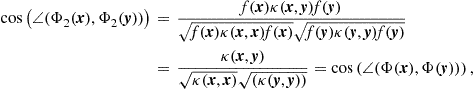
this transformation of the original kernel, preserves angles in the feature space. ![]()
Theorem 19
Restriction of a kernel
Let ![]() be a RKHS on X with respective kernel
be a RKHS on X with respective kernel ![]() . Then
. Then ![]() restricted to the set
restricted to the set ![]() is the reproducing kernel of the class
is the reproducing kernel of the class ![]() of all restrictions of functions of
of all restrictions of functions of ![]() to the subset
to the subset ![]() . The respective norm of any such restricted function
. The respective norm of any such restricted function ![]() (originating from
(originating from ![]() ) has norm
) has norm ![]() .
. ![]()
Proposition 20
Normalization of a kernel
Let ![]() be a RKHS on X with respective kernel
be a RKHS on X with respective kernel ![]() . Then
. Then
![]() (17.31)
(17.31)
is also a positive definite kernel on X. Note that ![]() , for all
, for all ![]() .
. ![]()
Proof
Let ![]() and
and ![]() be real numbers. Then
be real numbers. Then

as ![]() is a positive definite kernel.
is a positive definite kernel. ![]()
Theorem 21
Sum of kernels [3]
Let ![]() be two RKHS’s on X with respective kernels
be two RKHS’s on X with respective kernels ![]() . Then
. Then ![]() is also a reproducing kernel. The corresponding RKHS,
is also a reproducing kernel. The corresponding RKHS, ![]() , contains the functions
, contains the functions ![]() , where
, where ![]() . The respective norm is defined by
. The respective norm is defined by
![]()
![]()
Proof
It is trivial to show that ![]() is a positive definite kernel. The difficult part is to associate this kernel with the specific RKHS
is a positive definite kernel. The difficult part is to associate this kernel with the specific RKHS ![]() . Consider the Hilbert space
. Consider the Hilbert space ![]() . The respective inner product and the corresponding norm are defined as
. The respective inner product and the corresponding norm are defined as
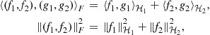
for ![]() and
and ![]() . If
. If ![]() and
and ![]() have only 0 in common, it easy to show that there is a one-to-one correspondence between F and
have only 0 in common, it easy to show that there is a one-to-one correspondence between F and ![]() , as each
, as each ![]() can be decomposed into two parts (one belonging to
can be decomposed into two parts (one belonging to ![]() and the other in
and the other in ![]() ) uniquely. The difficult part is to discover such a relation, if
) uniquely. The difficult part is to discover such a relation, if ![]() is larger than
is larger than ![]() . To make this fact clear, consider this simple example: Let
. To make this fact clear, consider this simple example: Let ![]() and
and ![]() be the linear classes of polynomials of orders up to 1 and up to 2 respectively. Obviously,
be the linear classes of polynomials of orders up to 1 and up to 2 respectively. Obviously, ![]() , as
, as ![]() . Let
. Let ![]() . Then f can be decomposed into two parts (one belonging to
. Then f can be decomposed into two parts (one belonging to ![]() and the other in
and the other in ![]() ) in more than one ways. For example
) in more than one ways. For example ![]() , or
, or ![]() , or
, or ![]() , e.t.c. Thus, the mapping between
, e.t.c. Thus, the mapping between ![]() and
and ![]() is not one-to-one. However, in such cases, we can still find a smaller subspace of F, which can be identified to
is not one-to-one. However, in such cases, we can still find a smaller subspace of F, which can be identified to ![]() .
.
To this end, define ![]() . It is clear that
. It is clear that ![]() is a linear subspace of F. We will show that it is a closed one. Consider the converging sequence in
is a linear subspace of F. We will show that it is a closed one. Consider the converging sequence in ![]() . Then
. Then ![]() and
and ![]() . Thus
. Thus ![]() and
and ![]() is in
is in ![]() . As
. As ![]() is a closed linear subspace of F, we may consider its complementary subspace
is a closed linear subspace of F, we may consider its complementary subspace ![]() .
.
As a next step, consider the linear transformation ![]() . The kernel of this transformation is the subspace
. The kernel of this transformation is the subspace ![]() . Hence, there is a one-to-one correspondence between
. Hence, there is a one-to-one correspondence between ![]() and
and ![]() . Consider the inverse transformation
. Consider the inverse transformation ![]() and let
and let ![]() , for
, for ![]() , where
, where ![]() and
and ![]() , i.e., through
, i.e., through ![]() we decompose f uniquely into two components, one in
we decompose f uniquely into two components, one in ![]() and the other in
and the other in ![]() . This decomposition enables us to define an inner product in
. This decomposition enables us to define an inner product in ![]() , i.e.,
, i.e.,
![]()
for ![]() . To prove that to this
. To prove that to this ![]() there corresponds the kernel
there corresponds the kernel ![]() , we make the following remarks:
, we make the following remarks:
![]()
and consequently ![]() . This means that
. This means that ![]() . Hence, for every
. Hence, for every ![]() we have
we have

As ![]() and
and ![]() , we conclude that
, we conclude that
![]()
This is the reproducing property.
Finally, to prove the last part of the theorem, consider again ![]() and let
and let ![]() , such that
, such that ![]() and let
and let ![]() and
and ![]() be the unique decomposition of f through
be the unique decomposition of f through ![]() . As
. As ![]() we obtain that
we obtain that ![]() , which implies that
, which implies that ![]() . Thus, we take:
. Thus, we take:

From the last relation we conclude that ![]() , if and only if
, if and only if ![]() and
and ![]() . In this case we take the minimum value of
. In this case we take the minimum value of ![]() , for all possible decompositions
, for all possible decompositions ![]() . This completes the proof.
. This completes the proof. ![]()
Despite the sum of kernels, other operations preserve reproducing kernels as well. Below, we give an extensive list of such operations. For a description of the induced RKHS and a formal proof (in the cases that are not considered here) the interested reader may refer to [3,13].
1. If ![]() is a positive definite kernel on X, then
is a positive definite kernel on X, then ![]() is also a positive definite kernel for any
is also a positive definite kernel for any ![]() . It is obvious that in this case
. It is obvious that in this case ![]() , if
, if ![]() . If
. If ![]() , then
, then ![]() .
.
2. If ![]() and
and ![]() are positive definite kernels on X, then
are positive definite kernels on X, then ![]() is also a positive definite kernel, as Theorem 21 established.
is also a positive definite kernel, as Theorem 21 established.
3. If ![]() and
and ![]() are positive definite kernels on X, then
are positive definite kernels on X, then ![]() is also a positive definite kernel.
is also a positive definite kernel.
4. If ![]() are positive definite kernels on X, such that
are positive definite kernels on X, such that ![]() , for all
, for all ![]() , then
, then ![]() is also a positive definite kernel.
is also a positive definite kernel.
5. If ![]() is a positive definite kernel on X and
is a positive definite kernel on X and ![]() is a polynomial with non-negative coefficients, then
is a polynomial with non-negative coefficients, then ![]() is also a positive definite kernel.
is also a positive definite kernel.
6. If ![]() is a positive definite kernel on X, then
is a positive definite kernel on X, then ![]() is also a positive definite kernel. To prove this, consider the Taylor expansion formula of
is also a positive definite kernel. To prove this, consider the Taylor expansion formula of ![]() , which may be considered as a limit of polynomials with non-negative coefficients.
, which may be considered as a limit of polynomials with non-negative coefficients.
7. If ![]() is a positive definite kernel on X and
is a positive definite kernel on X and ![]() is a function, then
is a function, then ![]() is a positive definite kernel on
is a positive definite kernel on ![]() .
.
8. If ![]() and
and ![]() are positive definite kernels on X and
are positive definite kernels on X and ![]() respectively, then their tensor product
respectively, then their tensor product ![]() , is a kernel on
, is a kernel on ![]() .
.
9. If ![]() and
and ![]() are positive definite kernels on X and
are positive definite kernels on X and ![]() respectively, then their direct sum
respectively, then their direct sum ![]() , is a kernel on
, is a kernel on ![]() .
.
1.17.5.6 Dot product and translation invariant kernels
There are two important classes of kernels that follow certain rules and are widely used in practice. The first one includes the dot product kernels, which are functions defined as ![]() , for some real function f. The second class are the translation invariant kernels, which are defined as
, for some real function f. The second class are the translation invariant kernels, which are defined as ![]() , for some real function f defined on X. The following theorems establish necessary and sufficient conditions for such functions to be reproducing kernels.
, for some real function f defined on X. The following theorems establish necessary and sufficient conditions for such functions to be reproducing kernels.
Theorem 22
Power Series of dot product kernels [29]
Let ![]() . A function
. A function ![]() defined on X, such that f has the power series expansion
defined on X, such that f has the power series expansion ![]() , is a positive definite kernel, if and only if we have
, is a positive definite kernel, if and only if we have ![]() for all n.
for all n. ![]()
Theorem 23
Bochner’s-Fourier Criterion for translation invariant kernels [20]
Let ![]() . A function
. A function ![]() defined on
defined on ![]() , is a positive definite kernel, if the Fourier transform
, is a positive definite kernel, if the Fourier transform
![]()
is non-negative. ![]()
Employing the tools provided in this section, one can readily prove the positivity of some of the kernels given in Section 1.17.5.4. For example:
• Homogeneous polynomial kernel: As ![]() is a positive definite kernel and
is a positive definite kernel and ![]() is a polynomial with non-negative coefficients,
is a polynomial with non-negative coefficients, ![]() is a positive definite kernel.
is a positive definite kernel.
• Inhomogeneous polynomial kernel: As ![]() is a positive definite kernel, and
is a positive definite kernel, and ![]() is a polynomial with non-negative coefficients (for positive c),
is a polynomial with non-negative coefficients (for positive c), ![]() is a positive definite kernel.
is a positive definite kernel.
• The cosine kernel: Note that ![]() . Thus the cosine kernel is the normalization of the simple kernel
. Thus the cosine kernel is the normalization of the simple kernel ![]() .
.
To prove that the Gaussian and the Laplacian are positive kernels we need another set of tools. This is the topic of Appendix A.
1.17.5.7 Differentiation in Hilbert spaces
1.17.5.7.1 Fréchet’s differentiation
In the following sections, we will develop cost functions defined on RKHS, that are suitable for minimization tasks related with adaptive filtering problems. As most minimization procedures involve computation of gradients or subgradients, we devote this section to study differentiation on Hilbert spaces. The notion of Fréchet’s Differentiability, which generalizes differentiability to general Hilbert spaces, lies at the core of this analysis.
Definition 25
Fréchet’s Differential
Let ![]() be a real Hilbert space,
be a real Hilbert space, ![]() a function, and
a function, and ![]() . The function
. The function ![]() is said to be Fréchet differentiable at f, if there exists a
is said to be Fréchet differentiable at f, if there exists a ![]() such that
such that
![]() (17.32)
(17.32)
where ![]() is the inner product of the Hilbert space
is the inner product of the Hilbert space ![]() and
and ![]() is the induced norm.
is the induced norm. ![]()
The element ![]() is called the gradient of the operator at f, and is usually denoted as
is called the gradient of the operator at f, and is usually denoted as ![]() . This relates to the standard gradient operator known by Calculus in Euclidean spaces. The Fréchet’s Differential is also known as Strong Differential. There is also a weaker definition of Differentiability, named Gâteaux’s Differential (or Weak Differential), which is a generalization of the directional derivative. The Gâteaux differential
. This relates to the standard gradient operator known by Calculus in Euclidean spaces. The Fréchet’s Differential is also known as Strong Differential. There is also a weaker definition of Differentiability, named Gâteaux’s Differential (or Weak Differential), which is a generalization of the directional derivative. The Gâteaux differential ![]() of
of ![]() at
at ![]() in the direction
in the direction ![]() is defined as
is defined as
![]() (17.33)
(17.33)
In the following, whenever we are referring to a derivative or a gradient we will mean the one produced by Fréchet’s notion of differentiability. The interested reader is addressed to [30–35], (amongst others) for a more detailed discussion on the subject. The well known properties of the derivative of a real valued function of one variable, which are known from elementary Calculus, like the product and chain rules, apply to the Fréchet’s derivatives as well.
The following simple examples demonstrate the differentiation procedure in arbitrary spaces.
Example 26
Consider the real Hilbert space ![]() , with inner product
, with inner product ![]() , and
, and ![]() , where
, where ![]() fixed. We can easily show (using Fréchet’s definition) that
fixed. We can easily show (using Fréchet’s definition) that ![]() is differentiable at any
is differentiable at any ![]() and that
and that ![]() . In the case where
. In the case where ![]() , we can easily show (using Fréchet’s definition) that
, we can easily show (using Fréchet’s definition) that ![]() is differentiable at any
is differentiable at any ![]() and that
and that ![]() .
.
1.17.6 Least squares learning algorithms
Having discussed the basic definitions and properties of RKHS we now turn to our main focus of the paper to discuss online learning schemes, which can operate in such spaces. We will start with two celebrated schemes, which are built around the Least Squares criterion, namely the LMS and the RLS.Although we can look at these algorithms as special cases of the schemes to be considered later on, in the more general setting of convex analytic tools, we chose to treat them separately. The reason is that the LMS and RLS are widely known, and the less familiar reader could follow their extension to RKHSs easier.
1.17.6.1 Least mean square (LMS)
Consider the sequence of examples ![]() , where
, where ![]() , and
, and ![]() for
for ![]() , and a parametric class of functions
, and a parametric class of functions ![]() . The goal of a typical online/adaptive learning task is to infer an input-output relationship
. The goal of a typical online/adaptive learning task is to infer an input-output relationship ![]() from the parametric class of functions
from the parametric class of functions ![]() , based on the given data, so that to minimize a certain loss function,
, based on the given data, so that to minimize a certain loss function, ![]() , that measures the error between the actual output,
, that measures the error between the actual output, ![]() , and the estimated output,
, and the estimated output, ![]() , at iteration n.
, at iteration n.
Least mean squares (LMS) algorithms are a popular class of adaptive learning systems that adopt the least mean squares error (i.e., the mean squared difference between the desired and the actual signal) to estimate the unknown coefficients ![]() . Its most typical form was invented in the 1960s by Bernard Widrow and his Ph.D. student Ted Hoff [36]. In the standard least mean square (LMS) setting, one adopts the class of linear functions, i.e.,
. Its most typical form was invented in the 1960s by Bernard Widrow and his Ph.D. student Ted Hoff [36]. In the standard least mean square (LMS) setting, one adopts the class of linear functions, i.e., ![]() and employs the mean square error,
and employs the mean square error, ![]() , as the loss function. To this end, the gradient descent rationale, e.g., [4–6], is employed and at each time instant,
, as the loss function. To this end, the gradient descent rationale, e.g., [4–6], is employed and at each time instant, ![]() , the gradient of the mean square error, i.e.,
, the gradient of the mean square error, i.e., ![]() , is approximated via its current measurement, i.e.,
, is approximated via its current measurement, i.e., ![]() , where
, where
![]()
If we define ![]() as the a-priori error, where
as the a-priori error, where ![]() is the current estimate, then the previous discussion leads naturally to the step update equation
is the current estimate, then the previous discussion leads naturally to the step update equation
![]() (17.34)
(17.34)
Another derivation of this classical recursion, through a convex analytic path, will be given in Section 1.17.7. Such a viewpoint will set the LMS as an instant of a larger family of algorithms.
Assuming that the initial ![]() , a repeated application of (17.34) gives
, a repeated application of (17.34) gives
![]() (17.35)
(17.35)
while the predicted output of the learning system at iteration n becomes
 (17.36)
There are a number of convergence criteria for the LMS algorithm [5]. Among the most popular ones are:
• The convergence of the mean property, i.e., ![]() , as
, as ![]() , where
, where ![]() and
and ![]() is the Wiener solution. Unfortunately, this is of little practical use, as any sequence of zero mean arbitrary random numbers converges in this sense.
is the Wiener solution. Unfortunately, this is of little practical use, as any sequence of zero mean arbitrary random numbers converges in this sense.
• The convergence in the mean square property: If the true input-output relation is given by ![]() , and
, and ![]() is a weakly stationary process, then
is a weakly stationary process, then ![]() , as
, as ![]() , provided that
, provided that ![]() satisfies the condition
satisfies the condition ![]() , where
, where ![]() is the largest eigenvalue of the correlation matrix
is the largest eigenvalue of the correlation matrix ![]() . We will see in Example 56 that the quantity
. We will see in Example 56 that the quantity ![]() stems also from a convex analytic point of view of the LMS-related estimation task. In practice, one usually uses
stems also from a convex analytic point of view of the LMS-related estimation task. In practice, one usually uses ![]() , where
, where ![]() denotes the trace of a matrix.
denotes the trace of a matrix.
• The Misadjustment property: The Misadjustment ratio, i.e., ![]() , where
, where
![]()
and ![]() is the minimum mean squared error associated with the optimum Wiener filter, is equal to
is the minimum mean squared error associated with the optimum Wiener filter, is equal to
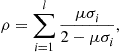
provided that the step update parameter ![]() satisfies
satisfies ![]() , where
, where ![]() are the eigenvalues of the correlation matrix
are the eigenvalues of the correlation matrix ![]() . This is a dimensionless quantity, providing a measure of closeness of the LMS algorithm from optimality in the mean square sense. The smallest
. This is a dimensionless quantity, providing a measure of closeness of the LMS algorithm from optimality in the mean square sense. The smallest ![]() is (compared to 1), the more accurate the learning system is. Usually
is (compared to 1), the more accurate the learning system is. Usually ![]() is expressed as a percentage. A misadjustment of
is expressed as a percentage. A misadjustment of ![]() is, ordinarily, considered to be satisfactory in practice [5].
is, ordinarily, considered to be satisfactory in practice [5].
LMS is sensitive to the scaling of the inputs ![]() . This makes it hard to choose a learning rate
. This makes it hard to choose a learning rate ![]() that guarantees the stability of the algorithm for various inputs. The Normalized LMS (NLMS) is a variant of the LMS designed to cope with this problem. It solves the problem by normalizing with the power of the input. Hence, the step update equation becomes
that guarantees the stability of the algorithm for various inputs. The Normalized LMS (NLMS) is a variant of the LMS designed to cope with this problem. It solves the problem by normalizing with the power of the input. Hence, the step update equation becomes
![]() (17.37)
(17.37)
where ![]() . It has been proved that the optimal learning rate of the NLMS is
. It has been proved that the optimal learning rate of the NLMS is ![]() [5,6]. We will also see in Section 1.17.7 that the NLMS has a clear geometrical interpretation; it is the repetition of a relaxed (metric) projection mapping onto a series of hyperplanes in the Euclidean space
[5,6]. We will also see in Section 1.17.7 that the NLMS has a clear geometrical interpretation; it is the repetition of a relaxed (metric) projection mapping onto a series of hyperplanes in the Euclidean space ![]() . More on the LMS family of algorithms, and more specifically, on its impact in modern signal processing, can be found in [4–6].
. More on the LMS family of algorithms, and more specifically, on its impact in modern signal processing, can be found in [4–6].
1.17.6.2 The Kernel LMS
In kernel-based algorithms, we estimate the output of the learning system by a nonlinear function f in a specific RKHS, ![]() , which is associated to a positive definite kernel
, which is associated to a positive definite kernel ![]() . The sequence of examples are transformed via the feature map
. The sequence of examples are transformed via the feature map ![]() ,
, ![]() and the LMS rationale is employed on the transforssmed data
and the LMS rationale is employed on the transforssmed data
![]()
while the estimated output at iteration n takes the form ![]() , for some
, for some ![]() . Although this is a linear algorithm in the RKHS
. Although this is a linear algorithm in the RKHS ![]() , it corresponds to a nonlinear processing in X. To calculate the gradient of the respective loss function,
, it corresponds to a nonlinear processing in X. To calculate the gradient of the respective loss function, ![]() , the Fréchet’s notion of differentiability is adopted, leading to:
, the Fréchet’s notion of differentiability is adopted, leading to: ![]() ; this, according to the LMS rationale, is approximated at each time instant by its current measurement, i.e.,
; this, according to the LMS rationale, is approximated at each time instant by its current measurement, i.e., ![]() . Consequently, following a gradient descent rationale, the step update equation of the KLMS is given by
. Consequently, following a gradient descent rationale, the step update equation of the KLMS is given by
![]() (17.38)
(17.38)
As it was stated for (17.34), the recursion (17.38) will be re-derived through convex analytic arguments in Section 1.17.7.
Assuming that ![]() , i.e., the zero function, a repeated application of (17.38) gives
, i.e., the zero function, a repeated application of (17.38) gives
![]() (17.39)
(17.39)
and the output of the filter at iteration n becomes
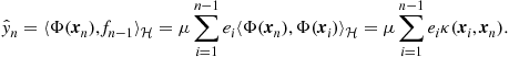 (17.40)
Equation (17.39) provides the KLMS estimate at time n. This is an expansion (in the RKHS ![]() ) in terms of the feature map function computed at each training point up to time n. Observe that, alternatively, one could derive Eq. (17.40), simply by applying the kernel trick to (17.36). It is important to emphasize that, in contrast to the standard LMS, where the solution is a vector of fixed dimension, which is updated at each time instant, in KLMS the solution is a function of
) in terms of the feature map function computed at each training point up to time n. Observe that, alternatively, one could derive Eq. (17.40), simply by applying the kernel trick to (17.36). It is important to emphasize that, in contrast to the standard LMS, where the solution is a vector of fixed dimension, which is updated at each time instant, in KLMS the solution is a function of ![]() and thus it cannot be represented by a machine. Nevertheless, as it is common in kernel-based methods, one needs not to compute the actual solution (17.39), but only the estimated output of the learning system,
and thus it cannot be represented by a machine. Nevertheless, as it is common in kernel-based methods, one needs not to compute the actual solution (17.39), but only the estimated output of the learning system, ![]() , which is given in terms of the kernel function centered at the points,
, which is given in terms of the kernel function centered at the points, ![]() , of the given sequence (Eq. (17.40)). Under this setting, the algorithm needs to store into memory two pieces of information: a) the centers (training input points),
, of the given sequence (Eq. (17.40)). Under this setting, the algorithm needs to store into memory two pieces of information: a) the centers (training input points), ![]() , of the expansion (17.39), which are stored into a dictionary
, of the expansion (17.39), which are stored into a dictionary ![]() and b) the coefficients of (17.39), i.e.,
and b) the coefficients of (17.39), i.e., ![]() , which are represented by a growing vector
, which are represented by a growing vector ![]() . Observe that (17.39) is inline with what we know by the Representer theorem given in Section 1.17.5 (Theorem 16). Algorithm 27 summarizes this procedure.
. Observe that (17.39) is inline with what we know by the Representer theorem given in Section 1.17.5 (Theorem 16). Algorithm 27 summarizes this procedure.
If in place of (17.38), we use its normalized version, i.e.,
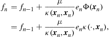 (17.41)

where ![]() , the normalized KLMS counterpart (KNLMS) results. This comprises replacing in Algorithm 27 the step
, the normalized KLMS counterpart (KNLMS) results. This comprises replacing in Algorithm 27 the step ![]() by
by ![]() , where
, where ![]() . The convergence and stability properties of KLMS is, still, a hot topic for research. One may consider that, as the KLMS is the LMS in a RKHS
. The convergence and stability properties of KLMS is, still, a hot topic for research. One may consider that, as the KLMS is the LMS in a RKHS ![]() , the properties of the LMS are directly transferred to the KLMS [37]. However, we should note that the properties of the LMS have been proved for Euclidean spaces, while very often the RKHS used in practice are of infinite dimension.
, the properties of the LMS are directly transferred to the KLMS [37]. However, we should note that the properties of the LMS have been proved for Euclidean spaces, while very often the RKHS used in practice are of infinite dimension.
1.17.6.2.1 Sparsifying the solution
The main drawback of the KLMS algorithm is that a growing number of training points, ![]() , is involved in the estimation of the learning system’s output (17.40). The set of these points can be thought of as a “dictionary,”
, is involved in the estimation of the learning system’s output (17.40). The set of these points can be thought of as a “dictionary,” ![]() , which is stored into the memory, as in Algorithm 27. This is a typical situation that arises in any kernel-based online learning scheme. As a consequence, increasing memory and computational resources are needed, as time evolves (the complexity of KLMS, as presented in Section 1.17.6.2 is
, which is stored into the memory, as in Algorithm 27. This is a typical situation that arises in any kernel-based online learning scheme. As a consequence, increasing memory and computational resources are needed, as time evolves (the complexity of KLMS, as presented in Section 1.17.6.2 is ![]() at each iteration). Furthermore, it is impossible to use the KLMS in real world’s applications, since the dictionary grows unbounded. In such a case, after a significant amount of iterations the expansion (17.40) will become so large that it will fill up the memory of the machine. In addition, it will require a huge amount of time to be computed, rendering the application useless. Hence, it is important to find a way to limit the size of this expansion. Several strategies have been proposed to cope with this problem. According to these strategies, the dictionary of points is created at the beginning of the algorithm and new points are inserted into it, only if they satisfy a specific rule, as in Algorithm 28. Adopting such a strategy, the complexity of KLMS is reduced to
at each iteration). Furthermore, it is impossible to use the KLMS in real world’s applications, since the dictionary grows unbounded. In such a case, after a significant amount of iterations the expansion (17.40) will become so large that it will fill up the memory of the machine. In addition, it will require a huge amount of time to be computed, rendering the application useless. Hence, it is important to find a way to limit the size of this expansion. Several strategies have been proposed to cope with this problem. According to these strategies, the dictionary of points is created at the beginning of the algorithm and new points are inserted into it, only if they satisfy a specific rule, as in Algorithm 28. Adopting such a strategy, the complexity of KLMS is reduced to ![]() , where
, where ![]() is the size of the dictionary at time instant n.
is the size of the dictionary at time instant n.
For example, in the popular Plat’s novelty criterion sparsification scheme [38], whenever a new data pair ![]() is considered, a decision is immediately made of whether to add the new point,
is considered, a decision is immediately made of whether to add the new point, ![]() , to
, to ![]() . The decision is reached following two simple rules:
. The decision is reached following two simple rules:
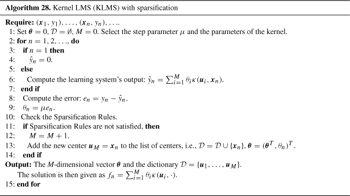
• First, the distance of the new point, ![]() , from the current dictionary,
, from the current dictionary, ![]() , is evaluated:
, is evaluated:
![]()
If this distance is smaller than a given threshold ![]() (i.e., the new input vector is close to a point, which is already in the existing dictionary), then the newly arrived point is not added to
(i.e., the new input vector is close to a point, which is already in the existing dictionary), then the newly arrived point is not added to ![]() . Thus
. Thus ![]() .
.
• Otherwise, we compute the prediction error ![]() . If
. If ![]() is smaller than a predefined threshold,
is smaller than a predefined threshold, ![]() , then the new point is discarded and we set
, then the new point is discarded and we set ![]() . Only if
. Only if ![]() , then
, then ![]() is inserted into
is inserted into ![]() , forming the new dictionary
, forming the new dictionary ![]() .
.
Note that whenever we insert a new point into ![]() , we must also insert the respective coefficient,
, we must also insert the respective coefficient, ![]() , to the growing vector
, to the growing vector ![]() .
.
Another popular scheme is the so called coherence-based sparsification strategy [39], where the point ![]() is inserted into the dictionary, if its coherence is above a given threshold
is inserted into the dictionary, if its coherence is above a given threshold ![]() , i.e.
, i.e.
![]() (17.42)
(17.42)
It has been proved that the dimension of the dictionary determined under rule (17.42) remains finite, as n goes to infinity [39].
A more sophisticated strategy is the so called surprise criterion [37], which employs ideas from information theoretic learning. The surprise of a new data pair ![]() with respect to a learning system
with respect to a learning system ![]() is defined as the negative log likelihood of
is defined as the negative log likelihood of ![]() , given the learning system’s hypothesis on the data distribution, i.e.,
, given the learning system’s hypothesis on the data distribution, i.e.,
![]()
According to this measure, one may classify the new data pair into the following three categories:
where ![]() are problem related parameters. In surprise-based sparsification, if the new data pair is classified as learnable, it is inserted into the dictionary. For the case of the KLMS with Gaussian inputs, the surprise measure is
are problem related parameters. In surprise-based sparsification, if the new data pair is classified as learnable, it is inserted into the dictionary. For the case of the KLMS with Gaussian inputs, the surprise measure is
![]() (17.43)
(17.43)
where
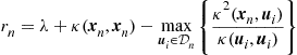
and ![]() is a user-defined regularization parameter.
is a user-defined regularization parameter.
A main drawback of the aforementioned sparsification techniques is that if one data point is inserted in the dictionary, it remains in it indefinitely. This may effect the tracking performance of the algorithm in time varying environments. Another technique, that one can adopt to impose sparsity on the solution of the KLMS, that, in addition, changes the coefficients of the solution’s expansion, is the quantization of the training data in the input space, as in the Quantized KLMS [40]. While each data point ![]() arrives sequentially, the algorithm checks if it is a new point or a redundant point. If its distance from the current dictionary
arrives sequentially, the algorithm checks if it is a new point or a redundant point. If its distance from the current dictionary ![]() is greater than or equal to the quantization size
is greater than or equal to the quantization size ![]() (i.e.,
(i.e., ![]() cannot be quantized to a point already contained in
cannot be quantized to a point already contained in ![]() ) then
) then ![]() is classified as a new point and it is inserted into the dictionary
is classified as a new point and it is inserted into the dictionary ![]() . Otherwise,
. Otherwise, ![]() is classified as a “redundant” point and the algorithm uses this information to update the coefficient of the closest center, say
is classified as a “redundant” point and the algorithm uses this information to update the coefficient of the closest center, say ![]() . Algorithm 29 summarizes this procedure.
. Algorithm 29 summarizes this procedure.
An alternative method to impose sparsity in an adaptive setting has been considered in [41–43]. This is based on regularization and it has the additional benefit of introducing an exponential forgetting mechanism of past data. This mechanism is very natural to the projection-based philosophy of these algorithms, and sparsification only requires an extra projection onto a convex ball.
1.17.6.2.2 Simulation results
To demonstrate the performance of the KLMS, we consider a typical nonlinear channel equalization task (see Figure 17.15) similar to the one presented in [44,45]. The nonlinear channel consists of a linear filter:
![]()
and a memoryless nonlinearity
![]() (17.44)
(17.44)

The signal is then corrupted by additive white Gaussian noise and then it is observed as ![]() . The level of the noise was set equal to 15 dB. The aim of a channel equalization task is to design an inverse filter, which acts on the output of the channel,
. The level of the noise was set equal to 15 dB. The aim of a channel equalization task is to design an inverse filter, which acts on the output of the channel, ![]() , and reproduces the original input signal,
, and reproduces the original input signal, ![]() , as close as possible. To this end, we apply the normalized KLMS algorithm to the set of samples
, as close as possible. To this end, we apply the normalized KLMS algorithm to the set of samples
![]() (17.45)
(17.45)
where ![]() is the equalizer’s length and D the equalization time delay, which is present to, almost, any equalization set up. In other words, the output of the equalizer at time n, provides the estimate of
is the equalizer’s length and D the equalization time delay, which is present to, almost, any equalization set up. In other words, the output of the equalizer at time n, provides the estimate of ![]() . This is to account for the non minimum phase property of the linear filter that was used to model the channel [5].
. This is to account for the non minimum phase property of the linear filter that was used to model the channel [5].
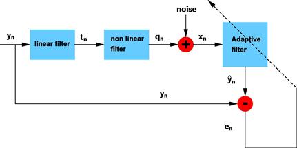
Experiments were conducted on 50 sets of 5000 samples of the input signal (Gaussian random variable with zero mean and unit variance) comparing the standard LMS and the KLMS. Regarding the KLMS, we employed the Gaussian kernel (with ![]() ) and we adopted the novelty criterion sparsification strategy
) and we adopted the novelty criterion sparsification strategy ![]() . The step update parameter,
. The step update parameter, ![]() , was tuned for the best possible results (in terms of the steady-state error rate). Time delay D was also set for optimality. Figure 17.16 shows the learning curves of KLMS versus the standard LMS algorithm. The superiority of the KLMS is evident and it was expected, since the standard LMS cannot cope with the nonlinearity.
, was tuned for the best possible results (in terms of the steady-state error rate). Time delay D was also set for optimality. Figure 17.16 shows the learning curves of KLMS versus the standard LMS algorithm. The superiority of the KLMS is evident and it was expected, since the standard LMS cannot cope with the nonlinearity.
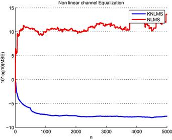
Figure 17.16 Learning curves of normalized LMS ![]() and the normalized Gaussian Kernel LMS
and the normalized Gaussian Kernel LMS ![]() for the equalization problem (filter length
for the equalization problem (filter length ![]() , delay
, delay ![]() ).
).
Figures 17.17a and 17.17b compare the performance of the various sparsification strategies presented in Section 1.17.6.2.1, considering the same experimental set up. The user-defined parameters for the novelty detection approach were set to ![]() , for the coherence-based scenario were set to
, for the coherence-based scenario were set to ![]() and for the surprise-based sparsification were set to
and for the surprise-based sparsification were set to ![]() . In this experiment, one observes that although both the surprise and the coherence-based scenarios perform almost equally well in terms of sparsity, the latter gives a slightly lower steady state MSE, whereas the novelty detection approach outperforms the other two both in terms of sparsity and the steady state MSE. Moreover, we should note that the coherence-based and the surprise strategies are more computationally demanding compared to the novelty criterion, as they involve several evaluations of the kernel function. Figure 17.18 compares the learning curves and the expansion’ size evolution of the QKLMS and the novelty detection KLMS at the same experimental set up. There it is shown that QKLMS, while offering a significant sparser solution, at the same time accomplishes a lower steady state MSE. In fact, the convergence behavior of QKLMS is almost identical to the KLMS without sparsification! Moreover, in terms of computational resources QKLMS is comparable to the novelty detection sparsification scenario.
. In this experiment, one observes that although both the surprise and the coherence-based scenarios perform almost equally well in terms of sparsity, the latter gives a slightly lower steady state MSE, whereas the novelty detection approach outperforms the other two both in terms of sparsity and the steady state MSE. Moreover, we should note that the coherence-based and the surprise strategies are more computationally demanding compared to the novelty criterion, as they involve several evaluations of the kernel function. Figure 17.18 compares the learning curves and the expansion’ size evolution of the QKLMS and the novelty detection KLMS at the same experimental set up. There it is shown that QKLMS, while offering a significant sparser solution, at the same time accomplishes a lower steady state MSE. In fact, the convergence behavior of QKLMS is almost identical to the KLMS without sparsification! Moreover, in terms of computational resources QKLMS is comparable to the novelty detection sparsification scenario.

Figure 17.17 (a) Learning curves of the normalized Kernel LMS (KNLMS) with ![]() , using the Gaussian kernel
, using the Gaussian kernel ![]() , under various sparsification strategies for the equalization problem (filter length
, under various sparsification strategies for the equalization problem (filter length ![]() , time delay
, time delay ![]() ). (b) Evolution of the expansion’s size at each time instant, for each sparsification strategy. The user-defined parameters for the novelty detection approach were set to
). (b) Evolution of the expansion’s size at each time instant, for each sparsification strategy. The user-defined parameters for the novelty detection approach were set to ![]() ,
, ![]() , for the coherence-based scenario were set to
, for the coherence-based scenario were set to ![]() and for the surprise-based sparsification were set to
and for the surprise-based sparsification were set to ![]() ,
, ![]() ,
, ![]() .
.

Figure 17.18 (a) Learning curves of the normalized Kernel LMS (KNLMS) with ![]() , using the Gaussian kernel
, using the Gaussian kernel ![]() , the novelty-detection normalized KNLMS and the QKLMS for the equalization problem (filter length
, the novelty-detection normalized KNLMS and the QKLMS for the equalization problem (filter length ![]() , time delay
, time delay ![]() ). (b) Evolution of the expansion’s size at each time instant, for the KNLMS, novelty KNLMS, QKNLMS. The user-defined parameters for the novelty detection approach were set to
). (b) Evolution of the expansion’s size at each time instant, for the KNLMS, novelty KNLMS, QKNLMS. The user-defined parameters for the novelty detection approach were set to ![]() ,
, ![]() . The quantization size (for the QKNLMS) was set
. The quantization size (for the QKNLMS) was set ![]() .
.
Finally, Figures 17.19 and 17.20 compare the performances of the aforementioned sparsification strategies in a set up where the channel undergoes a significant change. In this particular experiment, the input signal was fed to a channel consisting of the linear part ![]() and the nonlinear part
and the nonlinear part ![]() . The signal was then corrupted by additive white Gaussian noise and then observed as
. The signal was then corrupted by additive white Gaussian noise and then observed as ![]() . After the 2000th time instant the channel changes so that
. After the 2000th time instant the channel changes so that ![]() and
and ![]() . Experiments were conducted on 50 sets of 4000 samples of the input signal (Gaussian random variable with zero mean and unit variance). The QKLMS in this test gives excellent results, as it achieves the same steady state MSE as the unsparsified KLMS using only the 1/8th of the training centers. The three sparsification strategies (novelty, coherence, surprise) carry the information learned while the channel was in its original state throughout the learning phase. However, the two first (novelty and coherence) seem to be able to cope with the change of the channel, while the latter fails. The code for the experiments presented in this section can be found in http://bouboulis.mysch.gr/kernels.html. More simulation results for the KLMS algorithm are given in Sections 1.17.6.6.1 and 1.17.7.6.2, where it is validated against other kernel-based online learning methodologies, such as the Kernel RLS, and the projection-based Adaptive Projected Subgradient Method (APSM).
. Experiments were conducted on 50 sets of 4000 samples of the input signal (Gaussian random variable with zero mean and unit variance). The QKLMS in this test gives excellent results, as it achieves the same steady state MSE as the unsparsified KLMS using only the 1/8th of the training centers. The three sparsification strategies (novelty, coherence, surprise) carry the information learned while the channel was in its original state throughout the learning phase. However, the two first (novelty and coherence) seem to be able to cope with the change of the channel, while the latter fails. The code for the experiments presented in this section can be found in http://bouboulis.mysch.gr/kernels.html. More simulation results for the KLMS algorithm are given in Sections 1.17.6.6.1 and 1.17.7.6.2, where it is validated against other kernel-based online learning methodologies, such as the Kernel RLS, and the projection-based Adaptive Projected Subgradient Method (APSM).

Figure 17.19 (a) Learning curves of the normalized Kernel LMS (KNLMS) with ![]() , using the Gaussian kernel (
, using the Gaussian kernel (![]() ), under various sparsification strategies for the two states equalization problem (filter length
), under various sparsification strategies for the two states equalization problem (filter length ![]() , time delay
, time delay ![]() ). (b) Evolution of the expansion’s size at each time instant, for each sparsification strategy. The user-defined parameters for the novelty detection approach were set to
). (b) Evolution of the expansion’s size at each time instant, for each sparsification strategy. The user-defined parameters for the novelty detection approach were set to ![]() ,
, ![]() , for the coherence-based scenario were set to
, for the coherence-based scenario were set to ![]() and for the surprise-based sparsification were set to
and for the surprise-based sparsification were set to ![]() ,
, ![]() ,
, ![]() .
.

Figure 17.20 (a) Learning curves of the normalized Kernel LMS (KNLMS) with ![]() , using the Gaussian kernel
, using the Gaussian kernel ![]() , the novelty-detection normalized KNLMS and the QKLMS for the two-states equalization problem (filter length
, the novelty-detection normalized KNLMS and the QKLMS for the two-states equalization problem (filter length ![]() , time delay
, time delay ![]() ). (b) Evolution of the expansion’s size at each time instant, for the KNLMS, novelty KNLMS, QKNLMS. The user-defined parameters for the novelty detection approach were set to
). (b) Evolution of the expansion’s size at each time instant, for the KNLMS, novelty KNLMS, QKNLMS. The user-defined parameters for the novelty detection approach were set to ![]() ,
, ![]() . The quantization size (for the QKNLMS) was set
. The quantization size (for the QKNLMS) was set ![]() .
.
1.17.6.3 The complex case
Complex-valued signals arise frequently in applications as diverse as communications, bioinformatics, radar, etc. In this section we present the LMS rationale suitably adjusted to treat data of this nature.
1.17.6.3.1 Complex LMS
Let ![]() and
and ![]() be the input and the output of the original filter, respectively. In the typical Complex LMS (CLMS) rationale, we estimate the output of the filter using the so called
be the input and the output of the original filter, respectively. In the typical Complex LMS (CLMS) rationale, we estimate the output of the filter using the so called ![]() -linear function:
-linear function: ![]() . The CLMS aims to compute
. The CLMS aims to compute ![]() , such that the error
, such that the error ![]() is minimized. To compute the respective gradients, the notion of the Wirtinger’s Calculus [46,47] is employed as it simplifies calculations. In a nutshell, Wirtinger’s Calculus considers two types of derivatives, with respect to z and
is minimized. To compute the respective gradients, the notion of the Wirtinger’s Calculus [46,47] is employed as it simplifies calculations. In a nutshell, Wirtinger’s Calculus considers two types of derivatives, with respect to z and ![]() respectively (following the standard differentiation rules). However, only the second one is important for optimization tasks. The alternative to using Wirtinger’s calculus would be to consider the complex variables as pairs of two real ones and employ the common real partial derivatives. However, this approach, usually, is more time consuming and leads to more cumbersome expressions. Hence, applying the rules of Wirtinger’s calculus to this case, we take that
respectively (following the standard differentiation rules). However, only the second one is important for optimization tasks. The alternative to using Wirtinger’s calculus would be to consider the complex variables as pairs of two real ones and employ the common real partial derivatives. However, this approach, usually, is more time consuming and leads to more cumbersome expressions. Hence, applying the rules of Wirtinger’s calculus to this case, we take that ![]() , where
, where ![]() . Thus, the step update for the CLMS is
. Thus, the step update for the CLMS is
![]()
and the estimated output of the filter at iteration n, assuming that ![]() , is
, is
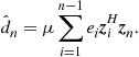
A different filtering structure has been brought to light more recently, mainly due to the works of Picinbono [48–50]. It is based on the notion of the widely linear estimation functions, where the output is estimated so that to be linear in terms of both z and ![]() , i.e.,
, i.e., ![]() . It turns out that the traditional approach to linearity, as employed by the CLMS, is rather “unorthodox,” as it excludes a large class of linear functions from being considered in the estimation process. Moreover, it can be shown that the correct complex linear estimation is the widely linear one [51]. In the context of the widely linear, or Augmented, CLMS (ACLMS), the vectors
. It turns out that the traditional approach to linearity, as employed by the CLMS, is rather “unorthodox,” as it excludes a large class of linear functions from being considered in the estimation process. Moreover, it can be shown that the correct complex linear estimation is the widely linear one [51]. In the context of the widely linear, or Augmented, CLMS (ACLMS), the vectors ![]() are computed, so that the error
are computed, so that the error ![]() is minimized. Applying Wirtinger’s Calculus we compute the respective gradients as
is minimized. Applying Wirtinger’s Calculus we compute the respective gradients as ![]() and
and ![]() . Thus, the step updates of the ACLMS become
. Thus, the step updates of the ACLMS become
![]() (17.46a)
(17.46a)
![]() (17.46b)
(17.46b)
and the estimated output at iteration n, assuming that ![]() , is
, is
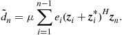 (17.47)
An important notion that has been associated with the case of complex data is the so called circularity. Circularity is intimately related to the rotation in the geometric sense. A complex random variable Z is called circular, if for any angle ![]() both Z and
both Z and ![]() (i.e., the rotation of Z by angle
(i.e., the rotation of Z by angle ![]() ) follow the same probability distribution [52,53]. It has been shown that, in the case of circular inputs, ACLMS and CLMS have identical performances [48,49,52,53]. However, ACLMS may show some performance gains when non-circular input sources are considered, although its convergence rate is somewhat slower than the CLMS. This is due to the fact that widely linear estimation processes are able to capture the full second-order statistics of a given complex signal, especially in the case where the signal is non-circular, by considering both the covariance and the pseudo-covariance matrices [49,50].
) follow the same probability distribution [52,53]. It has been shown that, in the case of circular inputs, ACLMS and CLMS have identical performances [48,49,52,53]. However, ACLMS may show some performance gains when non-circular input sources are considered, although its convergence rate is somewhat slower than the CLMS. This is due to the fact that widely linear estimation processes are able to capture the full second-order statistics of a given complex signal, especially in the case where the signal is non-circular, by considering both the covariance and the pseudo-covariance matrices [49,50].
1.17.6.3.2 Complex kernel LMS
Following a similar procedure, as the one adopted in the derivation of the KLMS from the standard LMS, kernel-based analogues of the CLMS can be produced. In general, to generate kernel adaptive filtering algorithms on complex domains, according to [54], one can adopt two methodologies. A first straightforward approach is to use directly a complex RKHS, using one of the complex kernels given in Section 1.17.5, and map the original data to the complex RKHS through the associated feature map ![]() . This is equivalent to applying the kernel trick to the standard complex LMS rationale in the usual black-box approach. Another alternative technique is to use real kernels through a rationale that is called complexification of real RKHSs. This method has the advantage of allowing modeling in complex RKHSs, using popular well-established and well understood, from a performance point of view, real kernels (e.g., Gaussian, polynomial, etc). While in the first case, we map the data directly to the complex RKHS through the feature map, in the complexification scenario we employ the map
. This is equivalent to applying the kernel trick to the standard complex LMS rationale in the usual black-box approach. Another alternative technique is to use real kernels through a rationale that is called complexification of real RKHSs. This method has the advantage of allowing modeling in complex RKHSs, using popular well-established and well understood, from a performance point of view, real kernels (e.g., Gaussian, polynomial, etc). While in the first case, we map the data directly to the complex RKHS through the feature map, in the complexification scenario we employ the map ![]() , where
, where ![]() , and
, and ![]() is the feature map of the chosen real kernel
is the feature map of the chosen real kernel ![]() , i.e.,
, i.e., ![]() . In the following, we will deal with the first scenario only. The complexification case is treated in [54].
. In the following, we will deal with the first scenario only. The complexification case is treated in [54].
Consider the complex RKHS ![]() , with the respective complex reproducing kernel
, with the respective complex reproducing kernel ![]() (meaning that it takes complex arguments and returns a complex number) defined on
(meaning that it takes complex arguments and returns a complex number) defined on ![]() , where
, where ![]() . We apply the feature map
. We apply the feature map ![]() of the RKHS,
of the RKHS, ![]() , to the points
, to the points ![]() and employ the LMS rationale to the transformed data
and employ the LMS rationale to the transformed data ![]() , modeling the desired output either as
, modeling the desired output either as ![]() , for some
, for some ![]() , or as
, or as ![]() , for some
, for some ![]() , if the more general widely linear approach is considered. In the first case, considering the corresponding loss as
, if the more general widely linear approach is considered. In the first case, considering the corresponding loss as ![]() , the Pure Complex KLMS (PCKLMS) is generated. To this end, the gradient descent rationale is adopted and the gradient of the loss function is estimated via its current measurement. To this end, Wirtinger’s calculus had to be generalized in the framework of Freshet derivation, to cope with infinite dimensional complex Hilbert spaces, [55]. It turns out that,
, the Pure Complex KLMS (PCKLMS) is generated. To this end, the gradient descent rationale is adopted and the gradient of the loss function is estimated via its current measurement. To this end, Wirtinger’s calculus had to be generalized in the framework of Freshet derivation, to cope with infinite dimensional complex Hilbert spaces, [55]. It turns out that, ![]() . This leads to the following step update equation:
. This leads to the following step update equation:
![]() (17.48)
(17.48)
Assuming that ![]() , and by applying a repetition of (17.48), we take formulas similar to the KLMS case. Algorithm 30 summarizes the procedure of PCKLMS.
, and by applying a repetition of (17.48), we take formulas similar to the KLMS case. Algorithm 30 summarizes the procedure of PCKLMS.
To sparsify the solution one may employ any of the methods described in Section 1.17.6.2.1. Adopting the widely linear estimation process, i.e., ![]() , and following a similar procedure, the Augmented Pure Complex KLMS (APCKLMS) is produced. In this case, as the corresponding loss is
, and following a similar procedure, the Augmented Pure Complex KLMS (APCKLMS) is produced. In this case, as the corresponding loss is ![]() , the respective estimation of gradients via their current measurements becomes
, the respective estimation of gradients via their current measurements becomes ![]() and
and ![]() . It turns out that the step update equations become:
. It turns out that the step update equations become:
![]()
The APCKLMS is treated in details in [51], where it is shown that it performs significantly better than the PCKLMS. The problem of complex estimation using kernels in the special case of finite dimensional Euclidean spaces has also been considered in [56].

1.17.6.4 Recursive Least Squares (RLS)
Recall that we assumed the sequence of examples ![]() , where
, where ![]() , and
, and ![]() . In the Recursive Least Squares (RLS) algorithm, we adopt the parametric class of linear functions, i.e.,
. In the Recursive Least Squares (RLS) algorithm, we adopt the parametric class of linear functions, i.e., ![]() , as the field in which we search for the optimal input-output relationship between
, as the field in which we search for the optimal input-output relationship between ![]() and
and ![]() , while the loss function at iteration n takes the form:
, while the loss function at iteration n takes the form:
![]() (17.49)
(17.49)
for some chosen ![]() . Observe that the loss function consists of two parts. The first one measures the error between the estimated output,
. Observe that the loss function consists of two parts. The first one measures the error between the estimated output, ![]() , and the actual output,
, and the actual output, ![]() , at each time instant, i, up to n, while the second is a regularization term. The existence of the second term is crucial to the algorithm, as it prevents it from being ill-posed and guards against overfitting. At each time instant, n, the RLS finds the solution to the minimization problem:
, at each time instant, i, up to n, while the second is a regularization term. The existence of the second term is crucial to the algorithm, as it prevents it from being ill-posed and guards against overfitting. At each time instant, n, the RLS finds the solution to the minimization problem:
![]() (17.50)
(17.50)
The RLS algorithm, usually, exhibits an order of magnitude faster convergence compared to the LMS, at the cost of higher computational complexity.
The rationale of the RLS algorithm can be described in a significant more compact form, if one adopts a matrix representation. To this end, we define the ![]() matrices
matrices ![]() and the vectors
and the vectors ![]() , for
, for ![]() . Then, the loss function (17.49) can be equivalently defined as:
. Then, the loss function (17.49) can be equivalently defined as:
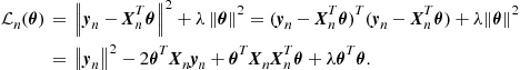
As this is a strictly convex function, it has a unique minimum, which it is obtained at the point, ![]() , where its gradient vanishes, i.e.,
, where its gradient vanishes, i.e., ![]() . Note, that the gradient of the loss function can be derived using standard differentiation rules:
. Note, that the gradient of the loss function can be derived using standard differentiation rules:
![]() (17.51)
(17.51)
Equating the gradient to zero, we obtain the solution to the minimization problem (17.50):
![]() (17.52)
(17.52)
where ![]() is the
is the ![]() identity matrix. Observe, that this solution includes the inversion of a matrix at each time step, which is usually, a computationally demanding procedure. To overcome this obstacle, the RLS algorithm computes the solution recursively, exploiting the matrix inversion lemma:
identity matrix. Observe, that this solution includes the inversion of a matrix at each time step, which is usually, a computationally demanding procedure. To overcome this obstacle, the RLS algorithm computes the solution recursively, exploiting the matrix inversion lemma:
![]() (17.53)
(17.53)
Let ![]() . Then, we can easily deduce that
. Then, we can easily deduce that ![]() . Thus, using the matrix inversion lemma (17.53) we take:
. Thus, using the matrix inversion lemma (17.53) we take:
![]()
Also, considering that ![]() , the solution
, the solution ![]() becomes
becomes
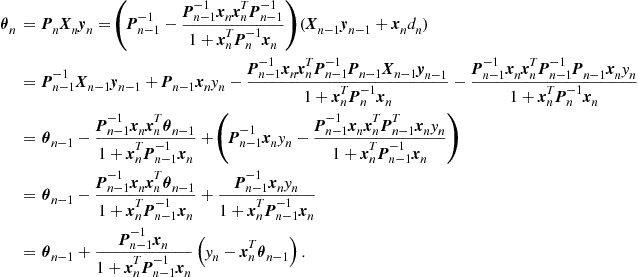
Thus, the solution ![]() is computed recursively, as
is computed recursively, as
![]() (17.54)
(17.54)
where ![]() is the estimation error at iteration n.
is the estimation error at iteration n.
As can be seen in Figure 17.21, which considers a 200-taps filter identification problem (where the input signal is a Gaussian random variable with zero mean and unit variance), the RLS learning procedure typically exhibits significantly faster convergence and achieves a lower steady state error compared to the NLMS (in this example the steady state MSE achieved by the RLS is 25% lower than the one achieved by the NLMS). Such a performance is expected for the stationary environment case. The RLS is a Newton-type algorithm and the LMS a gradient descent type. Moreover, concerning the excess error for the LMS, this is due to the non-diminishing value of ![]() , which as we know increases the steady state error.
, which as we know increases the steady state error.
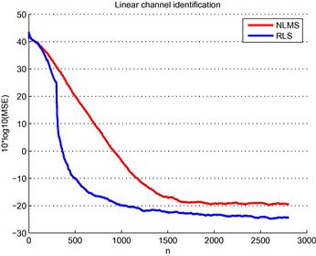
1.17.6.5 Exponentially weighted RLS
The RLS learning rationale utilizes information of all past data at each iteration step. Although this tactic enables RLS to achieve better convergence speed, it may become a burden in time-varying environments. In such cases, it would be preferable to simply “forget” some of the past data, which correspond to an earlier state of the learning task. We can incorporate such an approach to the RLS algorithm by introducing some weighting factors to the cost function (17.49), i.e.,
![]() (17.55)
(17.55)
where w is an appropriately chosen weighting function. A typical weighting scenario that is commonly used is the exponential weighting factor (or the forgetting factor), where we choose ![]() and
and ![]() , for some
, for some ![]() . Small values of w (close to 0) imply a strong forgetting mechanism, which makes the algorithm more sensitive to recent samples and might lead to poor performance. Hence, we usually select w such that it is close to 1. Obviously, for
. Small values of w (close to 0) imply a strong forgetting mechanism, which makes the algorithm more sensitive to recent samples and might lead to poor performance. Hence, we usually select w such that it is close to 1. Obviously, for ![]() we take the ordinary RLS described in 1.17.6.4. In the method of Exponentially Weighted RLS (EWRLS) we minimize the cost function
we take the ordinary RLS described in 1.17.6.4. In the method of Exponentially Weighted RLS (EWRLS) we minimize the cost function
![]() (17.56)
(17.56)
Using the matrix notation the aforementioned cost function becomes ![]() , where
, where ![]() and
and ![]() are defined as in Section 1.17.6.4 and
are defined as in Section 1.17.6.4 and ![]() is the diagonal matrix with elements the powers of w up to
is the diagonal matrix with elements the powers of w up to ![]() , i.e.,
, i.e.,

The solution to the respective minimization problem is
![]() (17.57)
(17.57)
Following a similar rationale as in Section 1.17.6.4, it turns out that:
![]()
and
![]()
Algorithm 31 describes the EWRLS machinery in details. We test the performance of the EWRLS in a time-varying channel identification problem. The signal (zero-mean unity-variance Gaussian random variable) is fed to a linear channel (length ![]() ) and then corrupted by white Gaussian noise. After 2000 samples of data, the coefficients of the linear channel undergo a significant change. Figure 17.22 shows the performance of the EWRLS algorithm compared to the standard RLS and the NLMS for
) and then corrupted by white Gaussian noise. After 2000 samples of data, the coefficients of the linear channel undergo a significant change. Figure 17.22 shows the performance of the EWRLS algorithm compared to the standard RLS and the NLMS for

1.17.6.6 The Kernel RLS
Similar to the case of the KLMS, in the Kernel RLS (KRLS) we estimate the learning system’s output by a function f defined on the RKHS, ![]() , which is associated to a positive definite kernel
, which is associated to a positive definite kernel ![]() . The sequence of examples are transformed via the feature map
. The sequence of examples are transformed via the feature map ![]() to generate the input data
to generate the input data
![]()
and the employed loss function takes the form
![]() (17.58)
(17.58)
The Representer Theorem 16 ensures that the solution to the minimization task, ![]() , lies in the finite dimensional subspace of the span of the n kernels that are centered on the training points
, lies in the finite dimensional subspace of the span of the n kernels that are centered on the training points ![]() . In other words:
. In other words:
![]() (17.59)
(17.59)
and thus, exploiting the kernel trick, the estimated output at iteration n will be given by
![]() (17.60)
(17.60)
As this expansion grows unbounded while time evolves, analogous to the case of KLMS, a sparsification mechanism, which keeps the most informative training points and discards the rest, is also needed. KRLS’s main task is to estimate the (growing) vector ![]() in a recursive manner.
in a recursive manner.
The first approach to the KRLS task was presented in [44] by Engel, Mannor, and Meir as a part of Engel’s Ph.D. thesis. Their method is built around a specific sparsification strategy, which is called Aproximate Linear Dependency (ALD). To this end, consider a dictionary of centers ![]() , of size
, of size ![]() , that keeps some of the past training points. In this setting, we test whether the newly arrived data
, that keeps some of the past training points. In this setting, we test whether the newly arrived data ![]() is approximately linearly dependent on the dictionary elements
is approximately linearly dependent on the dictionary elements ![]() . If not, we add it to the dictionary, otherwise
. If not, we add it to the dictionary, otherwise ![]() is approximated by a linear combination of the dictionary’s elements. The specific condition is whether
is approximated by a linear combination of the dictionary’s elements. The specific condition is whether
 (17.61)
where ![]() is a user-defined parameter. Using matrix-notation, this minimization problem can be equivalently recasted as:
is a user-defined parameter. Using matrix-notation, this minimization problem can be equivalently recasted as:
![]()
where ![]() , for
, for ![]() , and
, and ![]() . Assuming that
. Assuming that ![]() is invertible, the solution to this minimization problem is
is invertible, the solution to this minimization problem is
![]() (17.62)
(17.62)
while the attained minimum value is ![]() . In the case where
. In the case where ![]() ,
, ![]() is added to the dictionary, which now contains
is added to the dictionary, which now contains ![]() centers. If
centers. If ![]() , then
, then ![]() is not included to the dictionary, i.e.,
is not included to the dictionary, i.e., ![]() , and we approximate
, and we approximate ![]() as
as
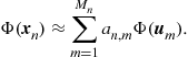 (17.63)
Using (17.63), we can approximate the full kernel matrix ![]() (i.e.,
(i.e., ![]() , for
, for ![]() ) as
) as
![]() (17.64)
(17.64)
where ![]() is the
is the ![]() matrix that contains the coefficients of the linear combinations associated with each
matrix that contains the coefficients of the linear combinations associated with each ![]() . This is due to the fact that at time index n each kernel evaluation is computed as
. This is due to the fact that at time index n each kernel evaluation is computed as

for all ![]() . Note that
. Note that ![]() for all
for all ![]() . This is the kick-off point of KRLS rationale.
. This is the kick-off point of KRLS rationale.
In matrix notation, the respective loss of the KRLS minimization task at iteration n is given by
![]()
As ![]() can be recasted as
can be recasted as
![]()
where ![]() is the new parameter to be optimized. Observe that while the original vector
is the new parameter to be optimized. Observe that while the original vector ![]() is a n-dimensional vector, the new vector,
is a n-dimensional vector, the new vector, ![]() , is significantly smaller (depending on the sparsification strategy). The solution to the modified minimization task is
, is significantly smaller (depending on the sparsification strategy). The solution to the modified minimization task is
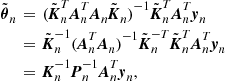 (17.65)
where ![]() , assuming that the inverse matrices exist. We distinguish the two different cases of the ALD sparsification and derive recursive relations for
, assuming that the inverse matrices exist. We distinguish the two different cases of the ALD sparsification and derive recursive relations for ![]() accordingly.
accordingly.
CASE I. If ![]() , then the data point arrived at iteration n, i.e.,
, then the data point arrived at iteration n, i.e., ![]() , is not added to the dictionary. Hence
, is not added to the dictionary. Hence ![]() and the expansion of
and the expansion of ![]() as a linear combination of the dictionary’s elements is added to
as a linear combination of the dictionary’s elements is added to ![]() , i.e.,
, i.e.,
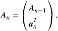 (17.66)
where ![]() is given by (17.62). Therefore,
is given by (17.62). Therefore, ![]() can be computed as
can be computed as
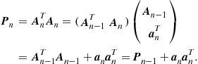
Applying the matrix inversion lemma, we take the recursive relation
![]() (17.67)
(17.67)
Substituting in (17.65) and considering that ![]() we take
we take

However, relation (17.65) implies that ![]() . Hence,
. Hence,
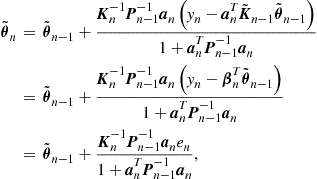
where the last relations are generated by substituting ![]() (see relation (17.62)) and considering that the estimated output at time index n by the learning system is
(see relation (17.62)) and considering that the estimated output at time index n by the learning system is ![]() .
.
CASE II. If ![]() , then the data point arrived at iteration n, i.e.,
, then the data point arrived at iteration n, i.e., ![]() , is added to the dictionary, i.e.,
, is added to the dictionary, i.e., ![]() and the matrices
and the matrices ![]() and
and ![]() are constructed as follows
are constructed as follows
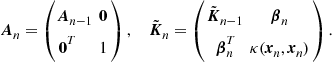
Moreover,

Hence, applying the matrix inversion lemma to ![]() and substituting
and substituting ![]() , we have
, we have

and

Observe that while we replace ![]() by
by ![]() using relation (17.62), the actual nth row of
using relation (17.62), the actual nth row of ![]() is
is ![]() . Substituting in (17.65) we take:
. Substituting in (17.65) we take:
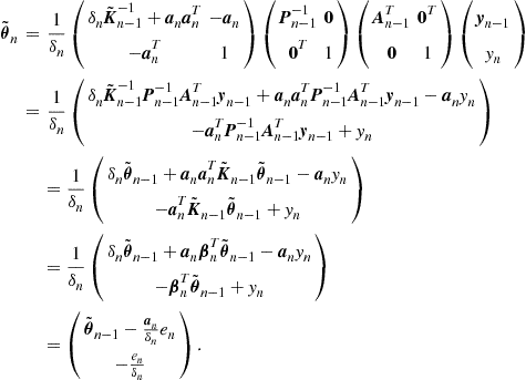
The procedure is summarized in Algorithm 32. The KRLS algorithm has complexity ![]() , at time n, where
, at time n, where ![]() is the size of the dictionary. Note, that we developed the specific recursive strategy assuming the invertibility of
is the size of the dictionary. Note, that we developed the specific recursive strategy assuming the invertibility of ![]() and
and ![]() for each n. For the case of the RKHS induced by the Gaussian kernel, which is the most popular kernel for practical applications, we can prove that
for each n. For the case of the RKHS induced by the Gaussian kernel, which is the most popular kernel for practical applications, we can prove that ![]() is indeed invertible. Furthermore, by construction, the matrix
is indeed invertible. Furthermore, by construction, the matrix ![]() has full-rank. Hence,
has full-rank. Hence, ![]() is strictly positive definite and thus invertible too.
is strictly positive definite and thus invertible too.
A methodology of similar spirit to the KRLS, which also takes advantage of the loss function (17.58) in the Support Vector Machines (SVM) rationale, can be found in [57–60]. An alternative path to the KRLS was followed in [61], via a formulation based on Gaussian Processes. Such an approach allows for an explicit forgetting factor mechanism to be incorporated in the adaptation flow. An alternative philosophy for forgetting past data in kernel-based adaptive schemes, in the framework of regularization, which can efficiently be implemented via projections, will be discussed in Section 1.17.7.