
Adaptive Filters
Vítor H. Nascimento and Magno T.M. Silva, Department of Electronic Systems Engineering, University of São Paulo, São Paulo, SP, Brazil, [email protected]
Abstract
This chapter provides an introduction to adaptive signal processing, covering basic principles through the most important recent developments. After a brief example for, we present an overview of how adaptive filters work, in which we use only deterministic arguments and concepts from basic linear systems theory, followed by a description of a few common applications of adaptive filters. Later, we turn to a more general model for adaptive filters based on stochastic processes and optimum estimation. Then three of the most important adaptive algorithms—LMS, NLMS, and RLS—are derived and analyzed in detail. The chapter closes with a brief description of some important extensions to the basic adaptive filtering algorithms and some promising current research topics. Since adaptive filter theory brings together results from several fields, short reviews are provided for most of the necessary material in separate sections, that the reader may consult if needed.
Keywords
Adaptive signal processing; Digital filters; Parameter estimation; Adaptive equalizers; Blind equalizers; Deconvolution; System identification; Echo cancellers
Acknowledgment
The authors thank Prof. Wallace A. Martins (Federal University of Rio de Janeiro) for his careful reading and comments on the text.
1.12.1 Introduction
Adaptive filters are employed in situations in which the environment is constantly changing, so that a fixed system would not have adequate performance. As they are usually applied in real-time applications, they must be based on algorithms that require a small number of computations per input sample.
These algorithms can be understood in two complementary ways. The most straightforward way follows directly from their name: an adaptive filter uses information from the environment and from the very signal it is processing to change itself, so as to optimally perform its task. The information from the environment may be sensed in real time (in the form of a so-called desired signal), or may be provided a priori, in the form of previous knowledge of the statistical properties of the input signal (as in blind equalization).
On the other hand, we can think of an adaptive filter also as an algorithm to separate a mixture of two signals. The filter must have some information about the signals to be able to separate them; usually this is given in the form of a reference signal, related to only one of the two terms in the mixture. The filter has then two outputs, corresponding to each signal in the mixture (see Figure 12.1). As a byproduct of separating the signals, the reference signal is processed in useful ways. This way of viewing an adaptive filter is very useful, particularly when one is learning the subject.

Figure 12.1 Inputs and outputs of an adaptive filter. Left: detailed diagram showing inputs, outputs and internal variable. Right: simplified diagram.
In the following sections we give an introduction to adaptive filters, covering from basic principles to the most important recent developments. Since the adaptive literature is vast, and the topic is still an active area of research, we were not able to treat all interesting topics. Along the text, we reference important textbooks, classic papers, and the most promising recent literature. Among the many very good textbooks on the subject, four of the most popular are [1–4].
We start with an application example, in the next section. In it, we show how an adaptive filter is applied to cancel acoustic echo in hands-free telephony. Along the text we return frequently to this example, to illustrate new concepts and methods. The example is completed by an overview of how adaptive filters work, in which we use only deterministic arguments and concepts from basic linear systems theory, in Section 1.12.1.2. This overview shows many of the compromises that arise in adaptive filter design, without the more complicated math. Section 1.12.1.3 gives a small glimpse of the wide variety of applications of adaptive filters, describing a few other examples. Of course, in order to fully understand the behavior of adaptive filters, one must use estimation theory and stochastic processes, which is the subject of Sections 1.12.2 and 1.12.3. The remaining sections are devoted to extensions to the basic algorithms and recent results.
Adaptive filter theory brings together results from several fields: signal processing, matrix analysis, control and systems theory, stochastic processes, and optimization. We tried to provide short reviews for most of the necessary material in separate links (“boxes”), that the reader may follow if needed.
1.12.1.1 Motivation—acoustic echo cancellation
Suppose that you are talking with a person who uses a hands-free telephone inside a car. Let us assume that the telephone does not have any acoustic echo canceler. In this case, the sound of your voice will reach the loudspeaker, propagate inside the car, and suffer reflections every time it encounters the walls of the car. Part of the sound can be absorbed by the walls, but part of it is reflected, resulting in an echo signal. This signal is fed back to the microphone and you will hear your own voice with delay and attenuation, as shown in Figure 12.2.
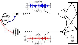
Figure 12.2 Echo in hands-free telephony. Click speech.wav to listen to a speech signal and echo.wav to listen to the corresponding echo signal.
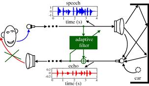
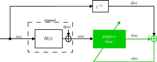
The echo signal depends on the acoustic characteristics of each car and also on the location of the loudspeaker and microphone. Furthermore, the acoustic characteristics can change during a phone call, since the driver may open or close a window, for example. In order to follow the variations of the environment, the acoustic echo must be canceled by an adaptive filter, which performs on-line updating of its parameters through an algorithm. Figure 12.3 shows the insertion of an adaptive filter in the system of Figure 12.2 to cancel the echo signal. In this configuration, the adaptive filter must identify the echo path and provide at its output an estimate of the echo signal. Thus, a synthesized version of the echo is subtracted from the signal picked up by the car microphone. In an ideal scenario, the resulting signal will be free of echo and will contain only the signal of interest. The general set-up of an echo canceler is shown in Figure 12.4. The near-end signal (near with respect to the echo canceler) may be simply noise when the person inside the car is in silence, as considered in Figures 12.2 and 12.3, or it can be a signal of interest, that is, the voice of the user in the car.

You most likely have already heard the output of an adaptive echo canceler. However, you probably did not pay attention to the initial period, when you can hear the adaptive filter learning the echo impulse response, if you listen carefully. We illustrate this through a simulation, using a measured impulse response of 256 samples (sampled at 8 kHz), and an echo signal produced from a recorded voice signal. The measured impulse response is shown in Figure 12.5. In the first example, the near-end signal is low-power noise (more specifically, white Gaussian noise with zero mean and variance ![]() ). Listen to e_nlms.wav, and pay attention to the beginning. You will notice that the voice (the echo) is fading away, while the adaptive filter is learning the echo impulse response. This file is the output of an echo canceler adapted using the normalized least-mean squares algorithm (NLMS), which is described in Section 1.12.3.2.
). Listen to e_nlms.wav, and pay attention to the beginning. You will notice that the voice (the echo) is fading away, while the adaptive filter is learning the echo impulse response. This file is the output of an echo canceler adapted using the normalized least-mean squares algorithm (NLMS), which is described in Section 1.12.3.2.

Listen now to e_lsl.wav in this case the filter was adapted using the modified error-feedback least-squares lattice algorithm (EF-LSL) [5], which is a low-cost and stable version of the recursive least-squares algorithm (RLS) described in Section 1.12.3.3. Now you will notice that the echo fades away much faster. This fast convergence is characteristic of the EF-LSL algorithm, and is of course a very desirable property. On the other hand, the NLMS algorithm is simpler to implement and more robust against imperfections in the implementation. An adaptive filtering algorithm must satisfy several requirements, such as convergence rate, tracking capability, noise rejection, computational complexity, and robustness. These requirements are conflicting, so that there is no best algorithm that will outperform all the others in every situation. The many algorithms available in the literature are different compromises between these requirements [1–3].
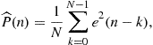
Figure 12.6 shows 4 s of the echo signal, prior to cancellation (bottom) and a measure of the quality of echo cancellation, the so-called echo return loss enhancement (ERLE) (top). The ERLE is defined as the ratio
![]()
The higher the ERLE, the better the performance of the canceler. The ERLE drops when the original echo is small (there is nothing to cancel!), and increases again when the echo is strong. The figure shows that EF-LSL performs better than NLMS (but at a higher computational cost).
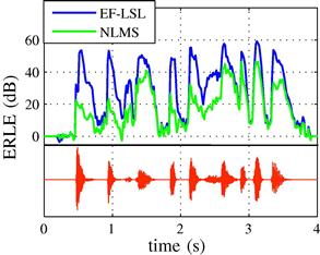
Figure 12.6 Echo return loss enhancement for NLMS ![]() and EF-LSL
and EF-LSL ![]() algorithms. Bottom trace: echo signal prior to cancellation. The meaning of the several parameters is explained in Sections 1.12.3.1, 1.12.3.2, and 1.12.3.3.
algorithms. Bottom trace: echo signal prior to cancellation. The meaning of the several parameters is explained in Sections 1.12.3.1, 1.12.3.2, and 1.12.3.3.
Assuming now that the near-end signal is another recorded voice signal (Click DT_echo.wav to listen to this signal), we applied again the EF-LSL algorithm to cancel the echo. This case simulates a person talking inside the car. Since the speech of this person is not correlated to the far-end signal, the output of the adaptive filter converges again to an estimate of the echo signal. Thus, a synthesized version of the echo is subtracted from the signal picked up by the car microphone and the resulting signal converges to the speech of the person inside the car. This result can be verified by listening to the file e_lslDT.wav.
This is a typical example of use of an adaptive filter. The environment (the echo impulse response) changes constantly, requiring a constant re-tuning of the canceling filter. Although the echo itself is not known, we have access to a reference signal (the clean speech of the far-end user). This is the signal that is processed to obtain an estimate of the echo. Finally, the signal captured by the near-end microphone (the so-called desired signal) is a mixture of two signals: the echo, plus the near-end speech (or ambient noise, when the near-end user is silent). The task of the adaptive filter can be seen as to separate these two signals.
We should mention that the name desired signal is somewhat misleading, although widespread in the literature. Usually we are interested in separating the “desired” signal into two parts, one of which is of no interest at all!
We proceed now to show how an algorithm can perform this task, modeling all signals as periodic to simplify the arguments.
1.12.1.2 A quick tour of adaptive filtering
Before embarking in a detailed explanation of adaptive filtering and its theory, it is a good idea to present the main ideas in a simple setting, to help the reader create intuition. In this section, we introduce the least-mean squares (LMS) algorithm and some of its properties using only deterministic arguments and basic tools from linear systems theory.
1.12.1.2.1 Posing the problem
Consider again the echo-cancellation problem, seen in the previous section (see Figure 12.7). Let ![]() represent the echo,
represent the echo, ![]() represent the voice of the near-end user, and
represent the voice of the near-end user, and ![]() the voice of the far-end user (the reference).
the voice of the far-end user (the reference). ![]() represents the signal that would be received by the far-end user without an echo canceler (the mixture, or desired signal).
represents the signal that would be received by the far-end user without an echo canceler (the mixture, or desired signal).
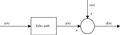
The echo path represents the changes that the far-end signal suffers when it goes through the digital-to-analog (D/A) converter, the loudspeaker, the air path between the loudspeaker and the microphone (including all reflections), the microphone itself and its amplifier, and the analog-to-digital (A/D) converter. The microphone signal ![]() will always be a mixture of the echo
will always be a mixture of the echo ![]() and an unrelated signal
and an unrelated signal ![]() , which is composed of the near-end speech plus noise. Our goal is to remove
, which is composed of the near-end speech plus noise. Our goal is to remove ![]() from
from ![]() . The challenge is that we have no means to measure
. The challenge is that we have no means to measure ![]() directly, and the echo path is constantly changing.
directly, and the echo path is constantly changing.
1.12.1.2.2 Measuring how far we are from the solution
How is the problem solved, then? Since we cannot measure ![]() , the solution is to estimate it from the measurable signals
, the solution is to estimate it from the measurable signals ![]() and
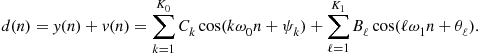
and ![]() . This is done as follows: imagine for now that all signals are periodic, so they can be decomposed as Fourier series
. This is done as follows: imagine for now that all signals are periodic, so they can be decomposed as Fourier series
 (12.1)
for certain amplitudes ![]() and
and ![]() , phases
, phases ![]() and
and ![]() , and frequencies
, and frequencies ![]() and
and ![]() . The highest frequencies appearing in
. The highest frequencies appearing in ![]() and
and ![]() must satisfy
must satisfy ![]() ,
, ![]() , since we are dealing with sampled signals (Nyquist criterion). We assume for now that the echo path is fixed (not changing), and can be modeled by an unknown linear transfer function
, since we are dealing with sampled signals (Nyquist criterion). We assume for now that the echo path is fixed (not changing), and can be modeled by an unknown linear transfer function ![]() . In this case,
. In this case, ![]() would also be a periodic sequence with fundamental frequency
would also be a periodic sequence with fundamental frequency ![]() ,
,

with ![]() . The signal picked by the microphone is then
. The signal picked by the microphone is then
Since we know ![]() , if we had a good approximation
, if we had a good approximation ![]() to
to ![]() , we could easily obtain an approximation
, we could easily obtain an approximation ![]() to
to ![]() and subtract it from
and subtract it from ![]() , as in Figure 12.8.
, as in Figure 12.8.
How could we find ![]() in real time? Recall that only
in real time? Recall that only ![]() , and
, and ![]() can be observed. For example, how could we know that we have the exact filter, that is, that
can be observed. For example, how could we know that we have the exact filter, that is, that ![]() , by looking only at these signals? To answer this question, take a closer look at
, by looking only at these signals? To answer this question, take a closer look at ![]() . Let the output of
. Let the output of ![]() be
be
 (12.2)
Assuming that the cosines in ![]() and
and ![]() have no frequencies in common, the simplest approach is to measure the average power of
have no frequencies in common, the simplest approach is to measure the average power of ![]() . Indeed, if all frequencies
. Indeed, if all frequencies ![]() and
and ![]() appearing in
appearing in ![]() are different from one another, then the average power of
are different from one another, then the average power of ![]() is
is
 (12.3)
If ![]() , then
, then ![]() is at its minimum,
is at its minimum,

which is the average power of ![]() . In this case,
. In this case, ![]() is at its optimum:
is at its optimum: ![]() , and the echo is completely canceled.
, and the echo is completely canceled.
It is important to see that this works because the two signals we want to separate, ![]() and
and ![]() , are uncorrelated, that is, they are such that
, are uncorrelated, that is, they are such that
 (12.4)
This property is known as the orthogonality condition. A form of orthogonality condition will appear in general whenever one tries to minimize a quadratic function, as is the case here. This is discussed in more detail in Section 1.12.2.
The average power ![]() could then be used as a measure of how good is our approximation
could then be used as a measure of how good is our approximation ![]() . The important point is that it is very easy to find a good approximation to
. The important point is that it is very easy to find a good approximation to ![]() . It suffices to low-pass filter
. It suffices to low-pass filter ![]() , for example,
, for example,
 (12.5)
is a good approximation if the window length ![]() is large enough.
is large enough.
The adaptive filtering problem then becomes an optimization problem, with the particularity that the cost function that is being minimized is not known exactly, but only through an approximation, as in (12.5). In the following sections, we discuss in detail the consequences of this fact.
It is also important to remark that the average error power is not the only possible choice for cost function. Although it is the most popular choice for a number of reasons, in some applications other choices are more adequate. Even posing the adaptive filtering problem as an optimization problem is not the only alternative, as shown by recent methods based on projections on convex sets [6].
1.12.1.2.3 Choosing a structure for the filter
Our approximation ![]() will be built by minimizing the estimated average error power (12.5) as a function of the echo path model
will be built by minimizing the estimated average error power (12.5) as a function of the echo path model ![]() , that is, our estimated echo path will be the solution of
, that is, our estimated echo path will be the solution of
![]() (12.6)
(12.6)
Keep in mind that we are looking for a real-time way of solving (12.6), since ![]() can only be obtained by measuring
can only be obtained by measuring ![]() for a certain amount of time. We must then be able to implement the current approximation
for a certain amount of time. We must then be able to implement the current approximation ![]() , so that
, so that ![]() and
and ![]() may be computed.
may be computed.
This will impose practical restrictions on the kind of function that ![]() may be: since memory and processing power are limited, we must choose beforehand a structure for
may be: since memory and processing power are limited, we must choose beforehand a structure for ![]() . Memory and processing power will impose a constraint on the maximum order the filter may have. In addition, in order to write the code for the filter, we must decide if it will depend on past outputs (IIR filters) or only on past inputs (FIR filters). These choices must be made based on some knowledge of the kind of echo path that our system is likely to encounter.
. Memory and processing power will impose a constraint on the maximum order the filter may have. In addition, in order to write the code for the filter, we must decide if it will depend on past outputs (IIR filters) or only on past inputs (FIR filters). These choices must be made based on some knowledge of the kind of echo path that our system is likely to encounter.
To explain how these choices can be made, let us simplify the problem a little more and restrict the far-end signal ![]() to a simple sinusoid (i.e., assume that
to a simple sinusoid (i.e., assume that ![]() ). In this case,
). In this case,
![]()
with ![]() . Therefore,
. Therefore, ![]() must satisfy
must satisfy
![]() (12.7)
(12.7)
only for ![]() —the value of
—the value of ![]() for other frequencies is irrelevant, since the input
for other frequencies is irrelevant, since the input ![]() has only one frequency. Expanding (12.7), we obtain
has only one frequency. Expanding (12.7), we obtain
![]() (12.8)
(12.8)
The optimum ![]() is defined through two conditions. Therefore an FIR filter with just two coefficients would be able to satisfy both conditions for any value of
is defined through two conditions. Therefore an FIR filter with just two coefficients would be able to satisfy both conditions for any value of ![]() , so we could define
, so we could define
![]()
and the values of ![]() and
and ![]() would be chosen to solve (12.6). Note that the argument generalizes for
would be chosen to solve (12.6). Note that the argument generalizes for ![]() : in general, if
: in general, if ![]() has
has ![]() harmonics, we could choose
harmonics, we could choose ![]() as an FIR filter with length
as an FIR filter with length ![]() , two coefficients per input harmonic.
, two coefficients per input harmonic.
This choice is usually not so simple: in practice, we would not know ![]() , and in the presence of noise (as we shall see later), a filter with fewer coefficients might give better performance, even though it would not completely cancel the echo. The structure of the filter also affects the dynamic behavior of the adaptive filter, so simply looking at equations such as (12.7) does not tell the whole story. Choosing the structure for
, and in the presence of noise (as we shall see later), a filter with fewer coefficients might give better performance, even though it would not completely cancel the echo. The structure of the filter also affects the dynamic behavior of the adaptive filter, so simply looking at equations such as (12.7) does not tell the whole story. Choosing the structure for ![]() is one of the most difficult steps in adaptive filter design. In general, the designer must test different options, initially perhaps using recorded signals, but ultimately building a prototype and performing some tests.
is one of the most difficult steps in adaptive filter design. In general, the designer must test different options, initially perhaps using recorded signals, but ultimately building a prototype and performing some tests.
1.12.1.2.4 Searching for the solution
Returning to our problem, assume then that we have decided that an FIR filter with length ![]() is adequate to model the echo path, that is,
is adequate to model the echo path, that is,
Our minimization problem (12.6) now reduces to finding the coefficients ![]() that solve
that solve
![]() (12.9)
(12.9)
Since ![]() must be computed from measurements, we must use an iterative method to solve (12.9). Many algorithms could be used, as long as they depend only on measurable quantities (
must be computed from measurements, we must use an iterative method to solve (12.9). Many algorithms could be used, as long as they depend only on measurable quantities (![]() , and
, and ![]() ). We will use the steepest descent algorithm (also known as gradient algorithm) as an example now. Later we show other methods that also could be used. If you are not familiar with the gradient algorithm, see Box 1 for an introduction.
). We will use the steepest descent algorithm (also known as gradient algorithm) as an example now. Later we show other methods that also could be used. If you are not familiar with the gradient algorithm, see Box 1 for an introduction.
The cost function in (12.9) is
We need to rewrite this equation so that the steepest descent algorithm can be applied. Recall also that now the filter coefficients will change, so define the vectors
![]()
and
![]()
where ![]() denotes transposition. At each instant, we have
denotes transposition. At each instant, we have ![]() , and our cost function becomes
, and our cost function becomes
 (12.10)
which depends on ![]() . In order to apply the steepest descent algorithm, let us keep the coefficient vector
. In order to apply the steepest descent algorithm, let us keep the coefficient vector ![]() constant during the evaluation of
constant during the evaluation of ![]() , as follows. Starting from an initial condition
, as follows. Starting from an initial condition ![]() , compute for
, compute for ![]() (The notation is explained in Boxes 2 and 6.)
(The notation is explained in Boxes 2 and 6.)
![]() (12.11)
(12.11)
where ![]() is a positive constant, and
is a positive constant, and ![]() . Our cost function now depends on only one
. Our cost function now depends on only one ![]() (compare with (12.10)):
(compare with (12.10)):
 (12.12)
We now need to evaluate the gradient of ![]() . Expanding the expression above, we obtain
. Expanding the expression above, we obtain

and
 (12.13)
As we needed, this gradient depends only on measurable quantities, ![]() and
and ![]() , for
, for ![]() . Our algorithm for updating the filter coefficients then becomes
. Our algorithm for updating the filter coefficients then becomes
 (12.14)
where we introduced the overall step-size ![]() .
.
We still must choose ![]() and
and ![]() . The choice of
. The choice of ![]() is more complicated and will be treated in Section 1.12.1.2.5. The value usually employed for
is more complicated and will be treated in Section 1.12.1.2.5. The value usually employed for ![]() may be a surprise: in almost all cases, one uses
may be a surprise: in almost all cases, one uses ![]() , resulting in the so-called least-mean squares (LMS) algorithm
, resulting in the so-called least-mean squares (LMS) algorithm
![]() (12.15)
(12.15)
proposed initially by Widrow and Hoff in 1960 [7] (Widrow [8] describes the history of the creation of the LMS algorithm). The question is, how can this work, if no average is being used for estimating the error power? An intuitive answer is not complicated: assume that ![]() is a very small number so that
is a very small number so that ![]() for a large
for a large ![]() . In this case, we can approximate
. In this case, we can approximate ![]() from (12.15) as follows.
from (12.15) as follows.
![]()
Since ![]() , we have
, we have ![]() . Therefore, we could approximate
. Therefore, we could approximate
![]()
so ![]() steps of the LMS recursion (12.15) would result
steps of the LMS recursion (12.15) would result
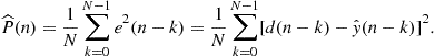
just what would be obtained from (12.14). The conclusion is that, although there is no explicit average being taken in the LMS algorithm (12.15), the algorithm in fact computes an implicit, approximate average if the step-size is small. This is exactly what happens, as can be seen in the animations in Figure 12.9. These simulations were prepared with
![]()
where ![]() and
and ![]() were chosen randomly in the interval
were chosen randomly in the interval ![]() . Several step-sizes were used. The estimates computed with the LMS algorithm are marked by the crosses (red in the web version). The initial condition is at the left, and the theoretical optimum is at the right end of each figure. In the simulations, the true echo path was modeled by the fixed filter
. Several step-sizes were used. The estimates computed with the LMS algorithm are marked by the crosses (red in the web version). The initial condition is at the left, and the theoretical optimum is at the right end of each figure. In the simulations, the true echo path was modeled by the fixed filter
![]()
For comparison, we also plotted the estimates that would be obtained by the gradient algorithm using the exact value of the error power at each instant. These estimates are marked with small dots (blue in the web version).
Figure 12.9 LMS algorithm for echo cancelation with sinusoidal input. Click LMS video files to see animations on your browser.
Note that when a small step-size is used, such as ![]() in Figure 12.9a, the LMS filter stays close to the dots obtained assuming exact knowledge of the error power. However, as the step-size increases, the LMS estimates move farther away from the dots. Although convergence is faster, the LMS estimates do not reach the optimum and stay there: instead, they hover around the optimum. For larger step-sizes, the LMS estimates can go quite far from the optimum (Figure 12.9b and c). Finally, if the step-size is too large, the algorithm will diverge, that is, the filter coefficients grow without bounds (Figure 12.9d).
in Figure 12.9a, the LMS filter stays close to the dots obtained assuming exact knowledge of the error power. However, as the step-size increases, the LMS estimates move farther away from the dots. Although convergence is faster, the LMS estimates do not reach the optimum and stay there: instead, they hover around the optimum. For larger step-sizes, the LMS estimates can go quite far from the optimum (Figure 12.9b and c). Finally, if the step-size is too large, the algorithm will diverge, that is, the filter coefficients grow without bounds (Figure 12.9d).
1.12.1.2.5 Tradeoff between speed and precision
The animations in Figure 12.9 illustrate an important problem in adaptive filters: even if you could magically chose as initial conditions the exact optimum solutions, the adaptive filter coefficients would not stay there! This happens because the filter does not know the exact value of the cost function it is trying to minimize (in this case, the error power): since ![]() is an approximation, noise (and the near-end signal in our echo cancellation example) would make the estimated gradient non-zero, and the filter would wander away from the optimum solution. This effect keeps the minimum error power obtainable using the adaptive filter always a little higher than the optimum value. The difference between the (theoretical, unattainable without perfect information) optimum and the actual error power is known as excess mean-square error (EMSE), and the ratio between the EMSE and the optimum error is known as misadjustment (see Eqs. (12.171) and (12.174)).
is an approximation, noise (and the near-end signal in our echo cancellation example) would make the estimated gradient non-zero, and the filter would wander away from the optimum solution. This effect keeps the minimum error power obtainable using the adaptive filter always a little higher than the optimum value. The difference between the (theoretical, unattainable without perfect information) optimum and the actual error power is known as excess mean-square error (EMSE), and the ratio between the EMSE and the optimum error is known as misadjustment (see Eqs. (12.171) and (12.174)).
For small step-sizes the misadjustment is small, since the LMS estimates stay close to the estimates that would be obtained with exact knowledge of the error power. However, a small step-size also means slow convergence. This trade-off exists in all adaptive filter algorithms, and has been an intense topic of research: many algorithms have been proposed to allow faster convergence without increasing the misadjustment. We will see some of them in the next sections.
The misadjustment is central to evaluate the performance of an adaptive filter. In fact, if we want to eliminate the echo from the near-end signal, we would like that after convergence, ![]() . This is indeed what happens when the step-size is small (see Figure 12.10a). However, when the step-size is increased, although the algorithm converges more quickly, the performance after convergence is not very good, because of the wandering of the filter weights around the optimum (Figure 12.10b–d—in the last case, for
. This is indeed what happens when the step-size is small (see Figure 12.10a). However, when the step-size is increased, although the algorithm converges more quickly, the performance after convergence is not very good, because of the wandering of the filter weights around the optimum (Figure 12.10b–d—in the last case, for ![]() , the algorithm is diverging.).
, the algorithm is diverging.).

Figure 12.10 Compromise between convergence rate and misadjustment in LMS. Plots of ![]() for several values of
for several values of ![]() .
.
We will stop this example here for the moment, and move forward to a description of adaptive filters using probability theory and stochastic processes. We will return to it during discussions of stability and model order selection.
The important message from this section is that an adaptive filter is able to separate two signals in a mixture by minimizing a well-chosen cost function. The minimization must be made iteratively, since the true value of the cost function is not known: only an approximation to it may be computed at each step. When the cost function is quadratic, as in the example shown in this section, the components of the mixture are separated such that they are in some sense orthogonal to each other.
Box 1:
Steepest descent algorithm
Given a cost function
![]()
with ![]() (
(![]() denotes transposition), we want to find the minimum of
denotes transposition), we want to find the minimum of ![]() , that is, we want to find
, that is, we want to find ![]() such that
such that
![]()
The solution can be found using the gradient of ![]() , which is defined by
, which is defined by

See Box 2 for a brief explanation about gradients and Hessians, that is, derivatives of functions of several variables.
The notation ![]() is most convenient when we deal with complex variables, as in Box 6. We use it for real variables for consistency.
is most convenient when we deal with complex variables, as in Box 6. We use it for real variables for consistency.
Since the gradient always points to the direction in which ![]() increases most quickly, the steepest descent algorithm searches iteratively for the minimum of
increases most quickly, the steepest descent algorithm searches iteratively for the minimum of ![]() taking at each iteration a small step in the opposite direction, i.e., towards
taking at each iteration a small step in the opposite direction, i.e., towards ![]() :
:
![]() (12.16)
(12.16)
where ![]() is a step-size, i.e., a constant controlling the speed of the algorithm. As we shall see, this constant should not be too small (or the algorithm will converge too slowly) neither too large (or the recursion will diverge).
is a step-size, i.e., a constant controlling the speed of the algorithm. As we shall see, this constant should not be too small (or the algorithm will converge too slowly) neither too large (or the recursion will diverge).
As an example, consider the quadratic cost function with ![]()
![]() (12.17)
(12.17)
with
 (12.18)
The gradient of ![]() is
is
![]() (12.19)
(12.19)
Of course, for this example we can find the optimum ![]() by equating the gradient to zero:
by equating the gradient to zero:
 (12.20)
Note that in this case the Hessian of ![]() (the matrix of second derivatives, see Box 2) is simply
(the matrix of second derivatives, see Box 2) is simply ![]() . As
. As ![]() is symmetric with positive eigenvalues
is symmetric with positive eigenvalues ![]() , it is positive-definite, and we can conclude that
, it is positive-definite, and we can conclude that ![]() is indeed a minimum of
is indeed a minimum of ![]() (See Boxes 2 and 3. Box 3 lists several useful properties of matrices.)
(See Boxes 2 and 3. Box 3 lists several useful properties of matrices.)
Even though in this case we could compute the optimum solution through (12.20), we will apply the gradient algorithm with the intention of understanding how it works and which are its main limitations. From (12.16) and (12.17), we obtain the recursion
![]() (12.21)
(12.21)
The user must choose an initial condition ![]() .
.
In Figure 12.11 we plot the evolution of the approximations computed through (12.21) against the level sets (i.e., curves of constant value) of the cost function (12.17). Different choices of step-size ![]() are shown. In Figure 12.11a, a small step-size is used. The algorithm converges to the correct solution, but slowly. In Figure 12.11b, we used a larger step-size—convergence is now faster, but the algorithm still needs several iterations to reach the solution. If we try to increase the step-size even further, convergence at first becomes slower again, with the algorithm oscillating towards the solution (Figure 12.11c). For even larger step-sizes, such as that in Figure 12.11d, the algorithm diverges: the filter coefficients get farther and farther away from the solution.
are shown. In Figure 12.11a, a small step-size is used. The algorithm converges to the correct solution, but slowly. In Figure 12.11b, we used a larger step-size—convergence is now faster, but the algorithm still needs several iterations to reach the solution. If we try to increase the step-size even further, convergence at first becomes slower again, with the algorithm oscillating towards the solution (Figure 12.11c). For even larger step-sizes, such as that in Figure 12.11d, the algorithm diverges: the filter coefficients get farther and farther away from the solution.

Figure 12.11 Performance of the steepest descent algorithm for different step-sizes. The crosses (x) represent the successive approximations ![]() , plotted against the level curves of (12.17). The initial condition is the point in the lower left.
, plotted against the level curves of (12.17). The initial condition is the point in the lower left.
It is important to find the maximum step-size for which the algorithm (12.21) remains stable. For this, we need concepts from linear systems and linear algebra, in particular eigenvalues, their relation to stability of linear systems, and the fact that symmetric matrices always have real eigenvalues (see Box 3).
The range of allowed step-sizes is found as follows. Rewrite (12.21) as
![]()
which is a linear recursion in state-space form (![]() is the identity matrix).
is the identity matrix).
Linear systems theory [9] tells us that this recursion converges as long as the largest eigenvalue of ![]() has absolute value less than one. The eigenvalues of
has absolute value less than one. The eigenvalues of ![]() are the roots of
are the roots of
![]()
Let ![]() . Then
. Then ![]() is an eigenvalue of
is an eigenvalue of ![]() if and only if
if and only if ![]() is an eigenvalue of
is an eigenvalue of ![]() . Therefore, if we denote by
. Therefore, if we denote by ![]() the eigenvalues of
the eigenvalues of ![]() , the stability condition is
, the stability condition is
![]()
The stability condition for our example is thus ![]() , in agreement with what we saw in Figure 12.11.
, in agreement with what we saw in Figure 12.11.
The gradient algorithm leads to relatively simple adaptive filtering algorithms; however, it has an important drawback. As you can see in Figure 12.11a, the gradient does not point directly to the direction of the optimum. This effect is heightened when the level sets of the cost function are very elongated, as in Figure 12.12. This case corresponds to a quadratic function in which ![]() has one eigenvalue much smaller than the other. In this example, we replaced the matrix
has one eigenvalue much smaller than the other. In this example, we replaced the matrix ![]() in (12.18) by
in (12.18) by

This matrix has eigenvalues ![]() and
and ![]() .
.

Figure 12.12 Performance of the steepest descent algorithm for a problem with large ratio of eigenvalues. The crosses (x) represent the successive approximations ![]() , plotted against the level curves of (12.17). The initial condition is the point in the lower left. Step-size
, plotted against the level curves of (12.17). The initial condition is the point in the lower left. Step-size ![]() .
.
Let us see why this is so. Recall from Box 3 that for every symmetric matrix there exists an orthogonal matrix ![]() (that is,
(that is, ![]() ) such that
) such that
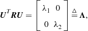 (12.22)
where we defined the diagonal eigenvalue matrix ![]() .
.
Let us apply a change of coordinates to (12.19). The optimum solution to (12.17) is
![]()
Our first change of coordinates is to replace ![]() by
by ![]() in (12.19). Subtract (12.19) from
in (12.19). Subtract (12.19) from ![]() and replace
and replace ![]() in (12.19) by
in (12.19) by ![]() to obtain
to obtain
![]() (12.23)
(12.23)
Next, multiply this recursion from both sides by ![]()
![]()
Defining ![]() , we have rewritten the gradient equation in a new set of coordinates, such that now the equations are uncoupled. Given that
, we have rewritten the gradient equation in a new set of coordinates, such that now the equations are uncoupled. Given that ![]() is diagonal, the recursion is simply
is diagonal, the recursion is simply
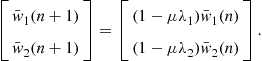 (12.24)
Note that, as long as ![]() for
for ![]() , both entries of
, both entries of ![]() will converge to zero, and consequently
will converge to zero, and consequently ![]() will converge to
will converge to ![]() .
.
The stability condition for this recursion is
![]()
When one of the eigenvalues is much larger than the other, say, when ![]() , the rate of convergence for the direction relative to the smaller eigenvalue becomes
, the rate of convergence for the direction relative to the smaller eigenvalue becomes
![]()
and even if one of the coordinates in ![]() converges quickly to zero, the other will converge very slowly. This is what we saw in Figure 12.12. The ratio
converges quickly to zero, the other will converge very slowly. This is what we saw in Figure 12.12. The ratio ![]() is known as the eigenvalue spread of a matrix.
is known as the eigenvalue spread of a matrix.
In general, the gradient algorithm converges slowly when the eigenvalue spread of the Hessian is large. One way of solving this problem is to use a different optimization algorithm, such as the Newton or quasi-Newton algorithms, which use the inverse of the Hessian matrix, or an approximation to it, to improve the search direction used by the gradient algorithm.
Although these algorithms converge very quickly, they require more computational power, compared to the gradient algorithm. We will see more about them when we describe the RLS (recursive least-squares) algorithm in Section 1.12.3.3.
For example, for the quadratic cost-function (12.17), the Hessian is equal to ![]() . If we had a good approximation
. If we had a good approximation ![]() to
to ![]() , we could use the recursion
, we could use the recursion
![]() (12.25)
(12.25)
This class of algorithms is known as quasi-Newton (if ![]() is an approximation) or Newton (if
is an approximation) or Newton (if ![]() is exact). In the Newton case, we would have
is exact). In the Newton case, we would have
![]()
that is, the algorithm moves at each step precisely in the direction of the optimum solution. Of course, this is not a very interesting algorithm for a quadratic cost function as in this example (the optimum solution is used in the recursion!) However, this method is very useful when the cost function is not quadratic and in adaptive filtering, when the cost function is not known exactly.
Box 2:
Gradients
Consider a function of several variables ![]() , where
, where

Its gradient is defined by
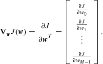
The real value of the notation ![]() will only become apparent when working with functions of complex variables, as shown in Box 6. We also define, for consistency,
will only become apparent when working with functions of complex variables, as shown in Box 6. We also define, for consistency,
![]()
As an example, consider the quadratic cost function
![]() (12.26)
(12.26)
The gradient of ![]() is (verify!)
is (verify!)
![]() (12.27)
(12.27)
If we use the gradient to find the minimum of ![]() , it would be necessary also to check the second-order derivative, to make sure the solution is not a maximum or a saddle point. The second order derivative of a function of several variables is a matrix, the Hessian. It is defined by
, it would be necessary also to check the second-order derivative, to make sure the solution is not a maximum or a saddle point. The second order derivative of a function of several variables is a matrix, the Hessian. It is defined by
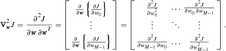 (12.28)
Note that for the quadratic cost-function (12.26), the Hessian is equal to ![]() . It is equal to
. It is equal to ![]() if
if ![]() is symmetric, that is, if
is symmetric, that is, if ![]() . This will usually be the case here. Note that
. This will usually be the case here. Note that ![]() is always symmetric: in fact, since for well-behaved functions
is always symmetric: in fact, since for well-behaved functions ![]() it holds that
it holds that
![]()
the Hessian is usually symmetric.
Assume that we want to find the minimum of ![]() . The first-order conditions are then
. The first-order conditions are then
![]()
The solution ![]() is a minimum of
is a minimum of ![]() if the Hessian at
if the Hessian at ![]() is a positive semi-definite matrix, that is, if
is a positive semi-definite matrix, that is, if
![]()
for all directions ![]() .
.
Box 3:
Useful results from Matrix Analysis
Here we list without proof a few useful results from matrix analysis. Detailed explanations can be found, for example, in [10–13].
Fact 1
Traces
The trace of a matrix ![]() is the sum of its diagonal elements:
is the sum of its diagonal elements:
 (12.29)
in which the ![]() are the entries of
are the entries of ![]() . For any two matrices
. For any two matrices ![]() and
and ![]() , it holds that
, it holds that
![]() (12.30)
(12.30)
In addition, if ![]() ,
, ![]() are the eigenvalues of a square matrix
are the eigenvalues of a square matrix ![]() , then
, then
 (12.31)
Fact 2
Singular matrices
A matrix ![]() is singular if and only if there exists a nonzero vector
is singular if and only if there exists a nonzero vector ![]() such that
such that ![]() .
.
The null space, or kernel![]() of a matrix
of a matrix ![]() is the set of vectors
is the set of vectors ![]() such that
such that ![]() . A square matrix
. A square matrix ![]() is nonsingular if, and only if,
is nonsingular if, and only if, ![]() , that is, if its null space contains only the null vector.
, that is, if its null space contains only the null vector.
Note that, if ![]() , with
, with ![]() , then
, then ![]() cannot be invertible if
cannot be invertible if ![]() . This is because when
. This is because when ![]() , there always exists a nonzero vector
, there always exists a nonzero vector ![]() such that
such that ![]() for
for ![]() , and thus
, and thus ![]() with
with ![]() .
.
Fact 3
Inverses of block matrices
Assume the square matrix ![]() is partitioned such that
is partitioned such that
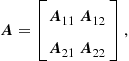
with ![]() and
and ![]() square. If
square. If ![]() and
and ![]() are invertible (nonsingular), then
are invertible (nonsingular), then
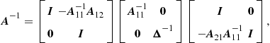
where ![]() is the Schur complement of
is the Schur complement of ![]() in
in ![]() . If
. If ![]() and
and ![]() are invertible, then
are invertible, then
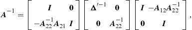
where ![]() .
.
Fact 4
Matrix inversion Lemma
Let ![]() and
and ![]() be two nonsingular
be two nonsingular ![]() matrices,
matrices, ![]() be also nonsingular, and
be also nonsingular, and ![]() be such that
be such that
![]() (12.32)
(12.32)
The inverse of ![]() is then given by
is then given by
![]() (12.33)
(12.33)
The lemma is most useful when ![]() . In particular when
. In particular when ![]() is a scalar, and we have
is a scalar, and we have
![]()
Fact 5
Symmetric matrices
Let ![]() be Hermitian Symmetric (or simply Hermitian), that is,
be Hermitian Symmetric (or simply Hermitian), that is, ![]() . Then, it holds that
. Then, it holds that
1. All eigenvalues ![]() ,
, ![]() of
of ![]() are real.
are real.
2. ![]() has a complete set of orthonormal eigenvectors
has a complete set of orthonormal eigenvectors ![]() ,
, ![]() . Since the eigenvectors are orthonormal,
. Since the eigenvectors are orthonormal, ![]() , where
, where ![]() if
if ![]() and 0 otherwise.
and 0 otherwise.
3. Arranging the eigenvectors in a matrix ![]() , we find that
, we find that ![]() is unitary, that is,
is unitary, that is, ![]() . In addition,
. In addition,

4. If ![]() , it is called simply symmetric. In this case, not only the eigenvalues, but also the eigenvectors are real.
, it is called simply symmetric. In this case, not only the eigenvalues, but also the eigenvectors are real.
Fact 6
Positive-definite matrices
If ![]() is Hermitian symmetric and moreover for all
is Hermitian symmetric and moreover for all ![]() it holds that
it holds that
![]() (12.34)
(12.34)
then ![]() is positive semi-definite. Positive semi-definite matrices have non-negative eigenvalues:
is positive semi-definite. Positive semi-definite matrices have non-negative eigenvalues: ![]() ,
, ![]() . They may be singular, if one or more eigenvalue is zero.
. They may be singular, if one or more eigenvalue is zero.
If the inequality (12.34) is strict, that is, if
![]() (12.35)
(12.35)
for all ![]() , then
, then ![]() is positive-definite. All eigenvalues
is positive-definite. All eigenvalues ![]() of positive-definite matrices satisfy
of positive-definite matrices satisfy ![]() . Positive-definite matrices are always nonsingular.
. Positive-definite matrices are always nonsingular.
Finally, all positive-definite matrices admit a Cholesky factorization, i.e., if ![]() is positive-definite, there is a lower-triangular matrix
is positive-definite, there is a lower-triangular matrix ![]() such that
such that ![]() [14].
[14].
Fact 7
Norms and spectral radius
The spectral radius![]() of a matrix
of a matrix ![]() is
is
![]() (12.36)
(12.36)
in which ![]() are the eigenvalues of
are the eigenvalues of ![]() . The spectral radius is important, because a linear system
. The spectral radius is important, because a linear system
![]()
is stable if and only if ![]() , as is well known. A useful inequality is that, for any matrix norm
, as is well known. A useful inequality is that, for any matrix norm ![]() such that for any
such that for any ![]()
![]()
it holds that
![]() (12.37)
(12.37)
This property is most useful when used with norms that are easy to evaluate, such as the 1-norm,
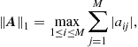
where ![]() are the entries of
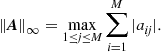
are the entries of ![]() . We could also use the infinity norm,
. We could also use the infinity norm,
1.12.1.3 Applications
Due to the ability to adjust themselves to different environments, adaptive filters can be used in different signal processing and control applications. Thus, they have been used as a powerful device in several fields, such as communications, radar, sonar, biomedical engineering, active noise control, modeling, etc. It is common to divide these applications into four groups:
In the first three cases, the goal of the adaptive filter is to find an approximation ![]() for the signal
for the signal ![]() , which is contained in the signal
, which is contained in the signal ![]() . Thus, as
. Thus, as ![]() approaches
approaches ![]() , the signal
, the signal ![]() approaches
approaches ![]() . The difference between these applications is in what we are interested. In interference cancellation, we are interested in the signal
. The difference between these applications is in what we are interested. In interference cancellation, we are interested in the signal ![]() , as is the case of acoustic echo cancellation, where
, as is the case of acoustic echo cancellation, where ![]() is the speech of the person using the hands-free telephone (go back to Figures 12.4 and 12.7). In system identification, we are interested in the filter parameters, and in prediction, we may be interested in the signal
is the speech of the person using the hands-free telephone (go back to Figures 12.4 and 12.7). In system identification, we are interested in the filter parameters, and in prediction, we may be interested in the signal ![]() and/or in the filter parameters. Note that in all these applications (interference cancellation, system identification and prediction), the signal
and/or in the filter parameters. Note that in all these applications (interference cancellation, system identification and prediction), the signal ![]() is an approximation for
is an approximation for ![]() and should not converge to zero, except when
and should not converge to zero, except when ![]() . In inverse system identification, differently from the other applications, the signal at the output of the adaptive filter must be as close as possible to the signal
. In inverse system identification, differently from the other applications, the signal at the output of the adaptive filter must be as close as possible to the signal ![]() and thus, ideally, the signal
and thus, ideally, the signal ![]() should be zeroed. In the sequel, we give an overview of these four groups in order to arrive at a common formulation that will simplify our analysis of adaptive filtering algorithms in further sections.
should be zeroed. In the sequel, we give an overview of these four groups in order to arrive at a common formulation that will simplify our analysis of adaptive filtering algorithms in further sections.
1.12.1.3.1 Interference cancellation
In a general interference cancellation problem, we have access to a signal ![]() , which is a mixture of two other signals,
, which is a mixture of two other signals, ![]() and
and ![]() . We are interested in one of these signals, and want to separate it from the other (the interference) (see Figure 12.13). Even though we do not know
. We are interested in one of these signals, and want to separate it from the other (the interference) (see Figure 12.13). Even though we do not know ![]() or
or ![]() , we have some information about
, we have some information about ![]() , usually in the form of a reference signal
, usually in the form of a reference signal ![]() that is related to
that is related to ![]() through a filtering operation
through a filtering operation ![]() . We may know the general form of this operation, for example, we may know that the relation is linear and well approximated by an FIR filter with 200 coefficients. However, we do not know the parameters (the filter coefficients) necessary to reproduce it. The goal of the adaptive filter is to find an approximation
. We may know the general form of this operation, for example, we may know that the relation is linear and well approximated by an FIR filter with 200 coefficients. However, we do not know the parameters (the filter coefficients) necessary to reproduce it. The goal of the adaptive filter is to find an approximation ![]() to
to ![]() , given only
, given only ![]() and
and ![]() . In the process of finding this
. In the process of finding this ![]() , the adaptive filter will construct an approximation for the relation
, the adaptive filter will construct an approximation for the relation ![]() . A typical example of an interference cancellation problem is the echo cancellation example we gave in Section 1.12.1.1. In that example,
. A typical example of an interference cancellation problem is the echo cancellation example we gave in Section 1.12.1.1. In that example, ![]() is the far-end voice signal,
is the far-end voice signal, ![]() is the near-end voice signal, and
is the near-end voice signal, and ![]() is the echo. The relation
is the echo. The relation ![]() is usually well approximated by a linear FIR filter with a few hundred taps.
is usually well approximated by a linear FIR filter with a few hundred taps.
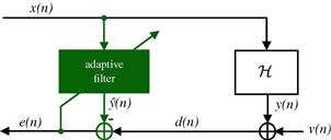
Figure 12.13 Scheme for interference cancellation and system identification. ![]() and
and ![]() are correlated to each other.
are correlated to each other.
The approximation for ![]() is a by-product, that does not need to be very accurate as long as it leads to a
is a by-product, that does not need to be very accurate as long as it leads to a ![]() close to
close to ![]() . This configuration is shown in Figure 12.13 and is called interference cancellation, since the interference
. This configuration is shown in Figure 12.13 and is called interference cancellation, since the interference ![]() should be canceled. Note that we do not want to make
should be canceled. Note that we do not want to make ![]() , otherwise we would not only be killing the interference
, otherwise we would not only be killing the interference ![]() , but also the signal of interest
, but also the signal of interest ![]() .
.
There are many applications of interference cancellation. In addition to acoustic and line echo cancellation, we can mention, for example, adaptive notch filters for cancellation of sinusoidal interference (a common application is removal of 50 or 60 Hz interference from the mains line), cancellation of the maternal electrocardiography in fetal electrocardiography, cancellation of echoes in long distance telephone circuits, active noise control (as in noise-canceling headphones), and active vibration control.
1.12.1.3.2 System identification
In interference cancellation, the coefficients of the adaptive filter converge to an approximation for the true relation ![]() , but as mentioned before, this approximation is a by-product that does not need to be very accurate. However, there are some applications in which the goal is to construct an approximation as accurate as possible for the unknown relation
, but as mentioned before, this approximation is a by-product that does not need to be very accurate. However, there are some applications in which the goal is to construct an approximation as accurate as possible for the unknown relation ![]() between
between ![]() and
and ![]() , thus obtaining a model for the unknown system. This is called system identification or modeling (the diagram in Figure 12.13 applies also for this case). The signal
, thus obtaining a model for the unknown system. This is called system identification or modeling (the diagram in Figure 12.13 applies also for this case). The signal ![]() is now composed of the output
is now composed of the output ![]() of an unknown system
of an unknown system ![]() , plus noise
, plus noise ![]() . The reference signal
. The reference signal ![]() is the input to the system which, when possible, is chosen to be white noise. In general, this problem is harder than interference cancellation, as we shall see in Section 1.12.2.1.5, due to some conditions that the reference signal
is the input to the system which, when possible, is chosen to be white noise. In general, this problem is harder than interference cancellation, as we shall see in Section 1.12.2.1.5, due to some conditions that the reference signal ![]() must satisfy. However, one point does not change: in the ideal case, the signal
must satisfy. However, one point does not change: in the ideal case, the signal ![]() will be equal to the noise
will be equal to the noise ![]() . Again, we do not want to make
. Again, we do not want to make ![]() , otherwise we would be trying to model the noise (however, the smaller the noise the easier the task, as one would expect).
, otherwise we would be trying to model the noise (however, the smaller the noise the easier the task, as one would expect).
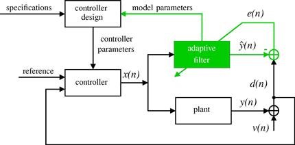
In many control systems, an unknown dynamic system (also called as plant in control system terminology) is identified online and the result is used in a self-tuning controller, as depicted in Figure 12.14. Both the plant and the adaptive filter have the same input ![]() . In practical situations, the plant to be modeled is noisy, which is represented by the signal
. In practical situations, the plant to be modeled is noisy, which is represented by the signal ![]() added to the plant output. The noise
added to the plant output. The noise ![]() is generally uncorrelated with the plant input. The task of the adaptive filter is to minimize the error model
is generally uncorrelated with the plant input. The task of the adaptive filter is to minimize the error model ![]() and track the time variations in the dynamics of the plant. The model parameters are continually fed back to the controller to obtain the controller parameters used in the self-tuning regulator loop [15].
and track the time variations in the dynamics of the plant. The model parameters are continually fed back to the controller to obtain the controller parameters used in the self-tuning regulator loop [15].
There are many applications that require the identification of an unknown system. In addition to control systems, we can mention, for example, the identification of the room impulse response, used to study the sound quality in concert rooms, and the estimation of the communication channel impulse response, required by maximum likelihood detectors and blind equalization techniques based on second-order statistics.
1.12.1.3.3 Prediction
In prediction, the goal is to find a relation between the current sample ![]() and previous samples
and previous samples ![]() , as shown in Figure 12.15. Therefore, we want to model
, as shown in Figure 12.15. Therefore, we want to model ![]() as a part
as a part ![]() that depends only on
that depends only on ![]() , and a part
, and a part ![]() that represents new information. For example, for a linear model, we would have
that represents new information. For example, for a linear model, we would have
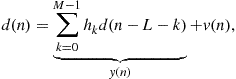
Thus, we in fact have again the same problem as in Figure 12.13. The difference is that now the reference signal is a delayed version of ![]() , and the adaptive filter will try to find an approximation
, and the adaptive filter will try to find an approximation ![]() for
for ![]() , thereby separating the “predictable” part
, thereby separating the “predictable” part ![]() of
of ![]() from the “new information”
from the “new information” ![]() , to which the signal
, to which the signal ![]() should converge. The system
should converge. The system ![]() in Figure 12.13 now represents the relation between
in Figure 12.13 now represents the relation between ![]() and the predictable part of
and the predictable part of ![]() .
.
Prediction finds application in many fields. We can mention, for example, linear predictive coding (LPC) and adaptive differential pulse code modulation (ADPCM) used in speech coding, adaptive line enhancement, autoregressive spectral analysis, etc.
For example, adaptive line enhancement (ALE) seeks the solution for a classical detection problem, whose objective is to separate a narrowband signal ![]() from a wideband signal
from a wideband signal ![]() . This is the case, for example, of finding a low-level sine wave (predictable narrowband signal) in noise (non-predictable wideband signal). The signal
. This is the case, for example, of finding a low-level sine wave (predictable narrowband signal) in noise (non-predictable wideband signal). The signal ![]() is constituted by the sum of these two signals. Using
is constituted by the sum of these two signals. Using ![]() as the reference signal and a delayed replica of it, i.e.,
as the reference signal and a delayed replica of it, i.e., ![]() , as input of the adaptive filter as in Figure 12.15, the output
, as input of the adaptive filter as in Figure 12.15, the output ![]() provides an estimate of the (predictable) narrowband signal
provides an estimate of the (predictable) narrowband signal ![]() , while the error signal
, while the error signal ![]() provides an estimate of the wideband signal
provides an estimate of the wideband signal ![]() . The delay
. The delay ![]() is also known as decorrelation parameter of the ALE, since its main function is to remove the correlation between the wideband signal
is also known as decorrelation parameter of the ALE, since its main function is to remove the correlation between the wideband signal ![]() present in the reference
present in the reference ![]() and in the delayed predictor input
and in the delayed predictor input ![]() .
.
1.12.1.3.4 Inverse system identification
Inverse system identification, also known as deconvolution, has been widely used in different fields as communications, acoustics, optics, image processing, control, among others. In communications, it is also known as channel equalization and the adaptive filter is commonly called as equalizer. Adaptive equalizers play an important role in digital communications systems, since they are used to mitigate the inter-symbol interference (ISI) introduced by dispersive channels. Due to its importance, we focus on the equalization application, which is explained in the sequel.
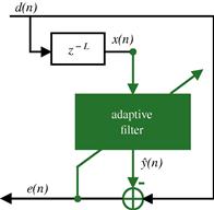
A simplified baseband communications system is depicted in Figure 12.16. The signal ![]() is transmitted through an unknown channel, whose model is constituted by an FIR filter with transfer function
is transmitted through an unknown channel, whose model is constituted by an FIR filter with transfer function ![]() and additive noise
and additive noise ![]() . Due to the channel memory, the signal at the receiver contains contributions not only from
. Due to the channel memory, the signal at the receiver contains contributions not only from ![]() , but also from the previous symbols
, but also from the previous symbols ![]() , i.e.,
, i.e.,
 (12.38)
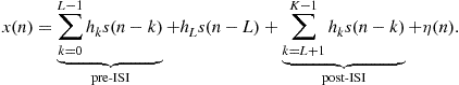
Assuming that the overall channel-equalizer system imposes a delay of ![]() samples, the adaptive filter will try to find an approximation
samples, the adaptive filter will try to find an approximation ![]() for
for ![]() and for this purpose, the two summations in (12.38), which constitute the inter-symbol interference, must be mitigated. Of course, when you are transmitting information the receiver will not have access to
and for this purpose, the two summations in (12.38), which constitute the inter-symbol interference, must be mitigated. Of course, when you are transmitting information the receiver will not have access to ![]() . The filter will adapt during a training phase, in which the transmitter sends a pre-agreed signal. You can see that in this case, the role of
. The filter will adapt during a training phase, in which the transmitter sends a pre-agreed signal. You can see that in this case, the role of ![]() and
and ![]() is the reverse of that in system identification. In this case, you would indeed like to have
is the reverse of that in system identification. In this case, you would indeed like to have ![]() . The problem is that this is not possible, given the presence of noise in
. The problem is that this is not possible, given the presence of noise in ![]() . The role of the adaptive filter is to approximately invert the effect of the channel, at the same time trying to suppress the noise (or at least, not to amplify it too much). In one sense, we are back to the problem of separating two signals, but now the mixture is in the reference signal
. The role of the adaptive filter is to approximately invert the effect of the channel, at the same time trying to suppress the noise (or at least, not to amplify it too much). In one sense, we are back to the problem of separating two signals, but now the mixture is in the reference signal ![]() , so what can and what cannot be done is considerably different from the other cases.
, so what can and what cannot be done is considerably different from the other cases.
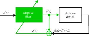
The scheme of Figure 12.16 is also called training mode, since the delayed version of the transmitted sequence ![]() (training sequence) is known at the receiver. After the convergence of the filter, the signal
(training sequence) is known at the receiver. After the convergence of the filter, the signal ![]() is changed to the estimate
is changed to the estimate ![]() obtained at the output of a decision device, as shown in Figure 12.17. In this case, the equalizer works in the so-called decision-directed mode. The decision device depends on the signal constellation—for example, if
obtained at the output of a decision device, as shown in Figure 12.17. In this case, the equalizer works in the so-called decision-directed mode. The decision device depends on the signal constellation—for example, if ![]() , the decision device returns
, the decision device returns ![]() for
for ![]() , and
, and ![]() for
for ![]() .
.
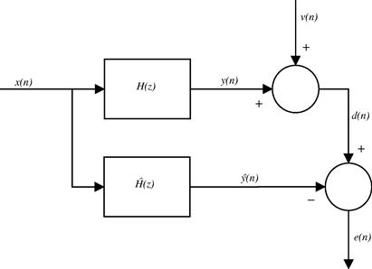
1.12.1.3.5 A common formulation
In all the four groups of applications, the inputs of the adaptive filter are given by the signals ![]() and
and ![]() and the output by
and the output by ![]() . Note that the input
. Note that the input ![]() appears effectively in the signal
appears effectively in the signal ![]() , which is computed and fed back at each time instant
, which is computed and fed back at each time instant ![]() , as shown in Figure 12.18. In the literature, the signal
, as shown in Figure 12.18. In the literature, the signal ![]() is referred to as desired signal,
is referred to as desired signal, ![]() as reference signal and
as reference signal and ![]() as error signal. These names unfortunately are somewhat misleading, since they give the impression that our goal is to recover exactly
as error signal. These names unfortunately are somewhat misleading, since they give the impression that our goal is to recover exactly ![]() by filtering (possibly in a nonlinear way) the reference
by filtering (possibly in a nonlinear way) the reference ![]() . In almost all applications, this is far from the truth, as previously discussed. In fact, except in the case of channel equalization, exactly zeroing the error would result in very poor performance.
. In almost all applications, this is far from the truth, as previously discussed. In fact, except in the case of channel equalization, exactly zeroing the error would result in very poor performance.

The only application in which ![]() is indeed a “desired signal” is channel equalization, in which
is indeed a “desired signal” is channel equalization, in which ![]() . Despite this particularity in channel equalization, the common feature in all adaptive filtering applications is that the filter must learn a relation between the reference
. Despite this particularity in channel equalization, the common feature in all adaptive filtering applications is that the filter must learn a relation between the reference ![]() and the desired signal
and the desired signal ![]() (we will use this name to be consistent with the literature.) In the process of building this relation, the adaptive filter is able to perform useful tasks, such as separating two mixed signals; or recovering a distorted signal. Section 1.12.2 explains this idea in more detail.
(we will use this name to be consistent with the literature.) In the process of building this relation, the adaptive filter is able to perform useful tasks, such as separating two mixed signals; or recovering a distorted signal. Section 1.12.2 explains this idea in more detail.
1.12.2 Optimum filtering
We now need to extend the ideas of Section 1.12.1.2, that applied only to periodic (deterministic) signals, to more general classes of signals. For this, we will use tools from the theory of stochastic processes. The main ideas are very similar: as before, we need to choose a structure for our filter and a means of measuring how far or how near we are to the solution. This is done by choosing a convenient cost function, whose minimum we must search iteratively, based only on measurable signals.
In the case of periodic signals, we saw that minimizing the error power (12.3), repeated below,

would be equivalent to zeroing the echo. However, we were not able to compute the error power exactly—we used an approximation through a time-average, as in (12.5), repeated here:
where ![]() is a convenient window length (in Section 1.12.1.2, we saw that choosing a large window length is approximately equivalent to choosing
is a convenient window length (in Section 1.12.1.2, we saw that choosing a large window length is approximately equivalent to choosing ![]() and a small step-size). Since we used an approximated estimate of the cost, our solution was also an approximation: the estimated coefficients did not converge exactly to their optimum values, but instead hovered around the optimum (Figures 12.9 and 12.10).
and a small step-size). Since we used an approximated estimate of the cost, our solution was also an approximation: the estimated coefficients did not converge exactly to their optimum values, but instead hovered around the optimum (Figures 12.9 and 12.10).
The minimization of the time-average ![]() also works in the more general case in which the echo is modeled as a random signal—but what is the corresponding exact cost function? The answer is given by the property of ergodicity that some random signals possess. If a random signal
also works in the more general case in which the echo is modeled as a random signal—but what is the corresponding exact cost function? The answer is given by the property of ergodicity that some random signals possess. If a random signal ![]() is such that its mean
is such that its mean ![]() does not depend on
does not depend on ![]() and its autocorrelation
and its autocorrelation ![]() depends only on
depends only on ![]() , it is called wide-sense stationary (WSS) [16]. If
, it is called wide-sense stationary (WSS) [16]. If ![]() is also (mean-square) ergodic, then
is also (mean-square) ergodic, then
 (12.39)
Note that ![]() is an ensemble average, that is, the expected value is computed over all possible realizations of the random signal. Relation (12.39) means that for an ergodic signal, the time average of a single realization of the process is equal to the ensemble-average of all possible realizations of the process. This ensemble average is the exact cost function that we would like to minimize.
is an ensemble average, that is, the expected value is computed over all possible realizations of the random signal. Relation (12.39) means that for an ergodic signal, the time average of a single realization of the process is equal to the ensemble-average of all possible realizations of the process. This ensemble average is the exact cost function that we would like to minimize.
In the case of adaptive filters, (12.39) holds approximately for ![]() for a finite value of
for a finite value of ![]() if the environment does not change too fast, and if the filter adapts slowly. Therefore, for random variables we will still use the average error power as a measure of how well the adaptive filter is doing. The difference is that in the case of periodic signals, we could understand the effect of minimizing the average error power in terms of the amplitudes of each harmonic in the signal, but now the interpretation will be in terms of ensemble averages (variances).
if the environment does not change too fast, and if the filter adapts slowly. Therefore, for random variables we will still use the average error power as a measure of how well the adaptive filter is doing. The difference is that in the case of periodic signals, we could understand the effect of minimizing the average error power in terms of the amplitudes of each harmonic in the signal, but now the interpretation will be in terms of ensemble averages (variances).
Although the error power is not the only possible choice for cost function, it is useful to study this choice in detail. Quadratic cost functions such as the error power have a number of properties that make them popular. For example, they are differentiable, and so it is relatively easy to find a closed-form solution for the optimum, and in the important case where all signals are Gaussian, the optimum filters are linear. Of course, quadratic cost functions are not the best option in all situations: the use of other cost functions, or even of adaptive filters not based on the minimization of a cost function, is becoming more common. We will talk about some of the most important alternatives in Sections 1.12.5.2 and 1.12.5.4.
Given the importance of quadratic cost functions, in this section we study them in detail. Our focus is on what could and what could not be done if the filter were able to measure perfectly ![]() at each instant. This discussion has two main goals: the first is to learn what is feasible, so we do not expect more from a filter than it can deliver. The second is to enable us to make more knowledgeable choices when designing a filter—for example, which filter order should be used, and for system identification, which input signal would result in better performance. In Section 1.12.4.4.3 we will study the performance of adaptive filters taking into consideration their imperfect knowledge of the environment.
at each instant. This discussion has two main goals: the first is to learn what is feasible, so we do not expect more from a filter than it can deliver. The second is to enable us to make more knowledgeable choices when designing a filter—for example, which filter order should be used, and for system identification, which input signal would result in better performance. In Section 1.12.4.4.3 we will study the performance of adaptive filters taking into consideration their imperfect knowledge of the environment.
1.12.2.1 Linear least-mean squares estimation
In the examples we gave in previous sections, a generic adaptive filtering problem resumed to this: we are given two sequences, ![]() and
and ![]() , as depicted in Figure 12.18. It is known, from physical arguments, that
, as depicted in Figure 12.18. It is known, from physical arguments, that ![]() has two parts, one that is in some sense related to
has two parts, one that is in some sense related to ![]() , and another that is not, and that both parts are combined additively, that is,
, and another that is not, and that both parts are combined additively, that is,
![]() (12.40)
(12.40)
where ![]() is an unknown relation, and
is an unknown relation, and ![]() is the part “unrelated” to
is the part “unrelated” to ![]() . In our examples so far,
. In our examples so far, ![]() was linear, but we do not need to restrict ourselves to this case. Our objective is to extract
was linear, but we do not need to restrict ourselves to this case. Our objective is to extract ![]() and
and ![]() from
from ![]() , based only on observations of
, based only on observations of ![]() and
and ![]() . We saw in Section 1.12.1.2 that the average power of the difference
. We saw in Section 1.12.1.2 that the average power of the difference ![]() between
between ![]() and our current approximation
and our current approximation ![]() could be used as a measure of how close we are to the solution. In general,
could be used as a measure of how close we are to the solution. In general, ![]() is time-variant, i.e., depends directly on
is time-variant, i.e., depends directly on ![]() . We will not write this dependence explicitly to simplify the notation.
. We will not write this dependence explicitly to simplify the notation.
In this section we ask in some sense the inverse problem, that is: given two sequences ![]() and
and ![]() , what sort of relation will be found between them if we use
, what sort of relation will be found between them if we use ![]() as a standard? The difference is that we now do not assume a model such as (12.40); instead, we want to know what kind of model results from the exact minimization of
as a standard? The difference is that we now do not assume a model such as (12.40); instead, we want to know what kind of model results from the exact minimization of ![]() , where
, where ![]() is defined as the difference between
is defined as the difference between ![]() and a function of
and a function of ![]()
We can answer this question in an entirely general way, without specifying beforehand the form of ![]() . This is done in Box 4. However, if we have information about the physics of a problem and know that the relation
. This is done in Box 4. However, if we have information about the physics of a problem and know that the relation ![]() is of a certain kind, we can restrict the search for the solution
is of a certain kind, we can restrict the search for the solution ![]() to this class. This usually reduces the complexity of the filter and increases its convergence rate (because less data is necessary to estimate a model with less unknowns, as we will see in Section 1.12.3). In this section we focus on this second option.
to this class. This usually reduces the complexity of the filter and increases its convergence rate (because less data is necessary to estimate a model with less unknowns, as we will see in Section 1.12.3). In this section we focus on this second option.
The first task is to describe the class ![]() of allowed functions
of allowed functions ![]() . This may be done by choosing a relation that depends on a few parameters, such as (recall that the adaptive filter output is
. This may be done by choosing a relation that depends on a few parameters, such as (recall that the adaptive filter output is ![]() )
)
![]() (12.41)
(12.41)
![]() (12.42)
(12.42)
 (12.43)
![]() (12.44)
(12.44)
In each of these cases, the relation between the input sequence ![]() and
and ![]() is constrained to a certain class, for example, linear length-
is constrained to a certain class, for example, linear length-![]() FIR filters in (12.41), first-order IIR filters in (12.42), and second-order Volterra filters in (12.43). Each class is described by a certain number of parameters: the filter coefficients
FIR filters in (12.41), first-order IIR filters in (12.42), and second-order Volterra filters in (12.43). Each class is described by a certain number of parameters: the filter coefficients ![]() in the case of FIR filters,
in the case of FIR filters, ![]() and
and ![]() in the case of IIR filters, and so on. The task of the adaptive filter will then be to choose the values of the parameters that best fit the data.
in the case of IIR filters, and so on. The task of the adaptive filter will then be to choose the values of the parameters that best fit the data.
For several practical reasons, it is convenient if we make the filter output depend linearly on the parameters, as happens in (12.41) and in (12.43). It is important to distinguish linear in the parameters from input-output linear: (12.43) is linear in the parameters, but the relation between the input sequence ![]() and the output
and the output ![]() is nonlinear. What may come as a surprise is that the IIR filter of Eq. (12.42) is not linear in the parameters: in fact,
is nonlinear. What may come as a surprise is that the IIR filter of Eq. (12.42) is not linear in the parameters: in fact, ![]() — you can see that
— you can see that ![]() depends nonlinearly on
depends nonlinearly on ![]() and
and ![]() .
.
Linearly parametrized classes ![]() , such as
, such as ![]() (12.41) and
(12.41) and ![]() (12.43) are popular because in general it is easier to find the optimum parameters, both theoretically and in real time. In fact, when the filter output depends linearly on the parameters and the cost function is a convex function of the error, it can be shown that the optimal solution is unique (see Box 5). This is a very desirable property, since it simplifies the search for the optimal solution.
(12.43) are popular because in general it is easier to find the optimum parameters, both theoretically and in real time. In fact, when the filter output depends linearly on the parameters and the cost function is a convex function of the error, it can be shown that the optimal solution is unique (see Box 5). This is a very desirable property, since it simplifies the search for the optimal solution.
In the remainder of this section we will concentrate on classes of relations that are linear in the parameters. As ![]() shows, this does not imply that we are restricting ourselves to linear models. There are, however, adaptive filtering algorithms that use classes of relations that are not linear in the parameters, such as IIR adaptive filters. On the other hand, blind equalization algorithms are based on non-convex cost functions.
shows, this does not imply that we are restricting ourselves to linear models. There are, however, adaptive filtering algorithms that use classes of relations that are not linear in the parameters, such as IIR adaptive filters. On the other hand, blind equalization algorithms are based on non-convex cost functions.
Assume then that we have chosen a convenient class of relations ![]() that depends linearly on its parameters. That is, we want to solve the problem
that depends linearly on its parameters. That is, we want to solve the problem
![]() (12.45)
(12.45)
We want to know which properties the solution to this problem will have when ![]() depends linearly on a finite number of parameters. In this case,
depends linearly on a finite number of parameters. In this case, ![]() is a linear combinations of certain functions
is a linear combinations of certain functions ![]() of
of ![]()
![]() (12.46)
(12.46)
where in general ![]() ,
, ![]() . The vector
. The vector ![]() is known as regressor. In the case of length-
is known as regressor. In the case of length-![]() FIR filters, we would have
FIR filters, we would have
![]()
whereas in the case of second-order Volterra filters with memory 1, we would have
![]()
Our problem can then be written in general terms as: find ![]() such that
such that
![]() (12.47)
(12.47)
We omitted the dependence of the variables on ![]() to lighten the notation. Note that, in general,
to lighten the notation. Note that, in general, ![]() will also depend on
will also depend on ![]() .
.
To solve this problem, we use the facts that ![]() to expand the expected value
to expand the expected value
![]()
Recall that the weight vector ![]() is not random, so we can take it out of the expectations.
is not random, so we can take it out of the expectations.
Define the autocorrelation of ![]() , and also the cross-correlation vector and autocorrelation matrix
, and also the cross-correlation vector and autocorrelation matrix
![]() (12.48)
(12.48)
The cost function then becomes
![]() (12.49)
(12.49)
Differentiating ![]() with respect to
with respect to ![]() , we obtain
, we obtain
![]()
and equating the result to zero, we see that the optimal solution must satisfy
![]() (12.50)
(12.50)
These are known as the normal, or Wiener-Hopf, equations. The solution, ![]() , is known as the Wiener solution. A note of caution: the Wiener solution is not the same thing as the Wiener filter. The Wiener filter is the linear filter that minimizes the mean-square error, without restriction of filter order [17]. The difference is that the Wiener solution has the filter order pre-specified (and is not restricted to linear filters, as we saw).
, is known as the Wiener solution. A note of caution: the Wiener solution is not the same thing as the Wiener filter. The Wiener filter is the linear filter that minimizes the mean-square error, without restriction of filter order [17]. The difference is that the Wiener solution has the filter order pre-specified (and is not restricted to linear filters, as we saw).
When the autocorrelation matrix is non-singular (which is usually the case), the Wiener solution is
![]() (12.51)
(12.51)
Given ![]() , the optimum error will be
, the optimum error will be
![]() (12.52)
(12.52)
Note that the expected value of ![]() is not necessarily zero:
is not necessarily zero:
![]() (12.53)
(12.53)
If, for example, ![]() and
and ![]() , then
, then ![]() . In practice, it is good to keep
. In practice, it is good to keep ![]() , because we usually know that
, because we usually know that ![]() should approximate a zero-mean signal, such as speech or noise. We will show shortly, in Section 1.12.2.1.4, how to guarantee that
should approximate a zero-mean signal, such as speech or noise. We will show shortly, in Section 1.12.2.1.4, how to guarantee that ![]() has zero mean.
has zero mean.
1.12.2.1.1 Orthogonality condition
A key property of the Wiener solution is that the optimum error is orthogonal to the regressor ![]() , that is,
, that is,
 (12.54)
We saw a similar condition in Section 1.12.1.2. It is very useful to remember this result, known as the orthogonality condition: from it, we will find when to apply the cost function (12.47) to design an adaptive filter. Note that when ![]() has zero mean, (12.54) also implies that
has zero mean, (12.54) also implies that ![]() and
and ![]() are uncorrelated.
are uncorrelated.
Remark 1
You should not confuse orthogonal with uncorrelated. Two random variables ![]() and
and ![]() are orthogonal if
are orthogonal if ![]() , whereas they are uncorrelated if
, whereas they are uncorrelated if ![]() . The two concepts coincide only if either
. The two concepts coincide only if either ![]() or
or ![]() have zero mean.
have zero mean.
Remark 2
The orthogonality condition is an intuitive result, if we remember that we can think of the space of random variables with finite variance as a vector space. In fact, define the cross-correlation ![]() between two random variables
between two random variables ![]() and
and ![]() as the inner product. Then the autocorrelation of a random variable
as the inner product. Then the autocorrelation of a random variable ![]() ,
, ![]() , would be interpreted as the square of the “length” of
, would be interpreted as the square of the “length” of ![]() . In this case, our problem (12.47) is equivalent to finding the vector in the subspace spanned by
. In this case, our problem (12.47) is equivalent to finding the vector in the subspace spanned by ![]() that is closest to
that is closest to ![]() . As we know, the solution is such that the error is orthogonal to the subspace. So, the orthogonality condition results from the vector space structure of our problem and the quadratic nature of our cost function. See Figure 12.19.
. As we know, the solution is such that the error is orthogonal to the subspace. So, the orthogonality condition results from the vector space structure of our problem and the quadratic nature of our cost function. See Figure 12.19.
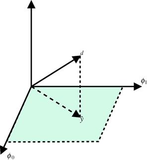
Remark 3
The difference between (12.54) and the corresponding result obtained in Box 4, Eq. (12.105), is that here the optimum error is orthogonal only to the functions ![]() of
of ![]() that were included in the regressor (and their linear combinations), not to any function, as in (12.105). This is not surprising: in this section the optimization was made only over the functions in class
that were included in the regressor (and their linear combinations), not to any function, as in (12.105). This is not surprising: in this section the optimization was made only over the functions in class ![]() , and in Box 4 we allow any function. Both solutions, (12.106) and (12.51), will be equal if the general solution according to Box 4 is indeed in
, and in Box 4 we allow any function. Both solutions, (12.106) and (12.51), will be equal if the general solution according to Box 4 is indeed in ![]() .
.
Remark 4
The optimal mean-square error is (recall that ![]() )
)
 (12.55)
Now that we have the general solution to (12.47), we turn to the question: for which class of problems is the quadratic cost function adequate?
1.12.2.1.2 Implicit vs. physical models
From (12.54), we see that the fact that we are minimizing the mean-square error between ![]() and a linear combination of the regressor
and a linear combination of the regressor ![]() induces a model
induces a model
![]() (12.56)
(12.56)
in which ![]() is orthogonal to
is orthogonal to ![]() . This is not an assumption, as we sometimes see in the literature, but a consequence of the quadratic cost function we chose. In other words, there is always a relation such as (12.56) between any pair
. This is not an assumption, as we sometimes see in the literature, but a consequence of the quadratic cost function we chose. In other words, there is always a relation such as (12.56) between any pair ![]() , as long as both have finite second-order moments. This relation may make sense from a physical analysis of the problem (as we saw in the echo cancellation example), or be simply a consequence of solving (12.47) (see Section 1.12.2.1.3 for examples).
, as long as both have finite second-order moments. This relation may make sense from a physical analysis of the problem (as we saw in the echo cancellation example), or be simply a consequence of solving (12.47) (see Section 1.12.2.1.3 for examples).
On the other hand, the orthogonality condition allows us to find out when the solution of (12.47) will be able to successfully solve a problem: assume now that we know beforehand, by physical arguments about the problem, that ![]() and
and ![]() must be related through
must be related through
![]() (12.57)
(12.57)
where ![]() is a certain coefficient vector and
is a certain coefficient vector and ![]() is orthogonal to
is orthogonal to ![]() . Will the solution to (12.47) be such that
. Will the solution to (12.47) be such that ![]() and
and ![]() ?
?
To check if this is the case, we only need to evaluate the cross-correlation vector ![]() assuming the model (12.57):
assuming the model (12.57):
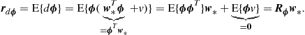 (12.58)
Therefore, ![]() also obeys the normal equations, and we can conclude that
also obeys the normal equations, and we can conclude that ![]() , as long as
, as long as ![]() is nonsingular.
is nonsingular.
Even if ![]() is singular, the optimal error
is singular, the optimal error ![]() will always be equal to
will always be equal to ![]() (in a certain sense). In fact, if
(in a certain sense). In fact, if ![]() is singular, then there exists a vector
is singular, then there exists a vector ![]() such that
such that ![]() (see Fact 2 in Box 3), and thus any solution
(see Fact 2 in Box 3), and thus any solution ![]() of the normal equations (we know from (12.58) that there is at least one,
of the normal equations (we know from (12.58) that there is at least one, ![]() ) will have the form
) will have the form
![]() (12.59)
(12.59)
where ![]() is the null-space of
is the null-space of ![]() . In addition,
. In addition,
![]()
Therefore, ![]() with probability one. Then,
with probability one. Then,
![]()
with probability one. Therefore, although we cannot say that ![]() always, we can say that they are equal with probability one. In other words, when
always, we can say that they are equal with probability one. In other words, when ![]() is singular we may not be able to identify
is singular we may not be able to identify ![]() , but (with probability one) we are still able to separate
, but (with probability one) we are still able to separate ![]() into its two components. More about this in Section 1.12.2.1.5.
into its two components. More about this in Section 1.12.2.1.5.
1.12.2.1.3 Undermodeling
We just saw that the solution to the quadratic cost function (12.47) is indeed able to separate the two components of ![]() when the regressor that appears in physical model (12.57) is the same
when the regressor that appears in physical model (12.57) is the same ![]() that we used to describe our class
that we used to describe our class ![]() , that is, when our choice of
, that is, when our choice of ![]() includes the general solution from Box 4. Let us check now what happens when this is not the case.
includes the general solution from Box 4. Let us check now what happens when this is not the case.
Assume there is a relation
![]() (12.60)
(12.60)
in which ![]() is orthogonal to
is orthogonal to ![]() , but our class
, but our class ![]() is defined through a regressor
is defined through a regressor ![]() that is a subset of the “correct” one,
that is a subset of the “correct” one, ![]() . This situation is called undermodeling: our class is not rich enough to describe the true relation between
. This situation is called undermodeling: our class is not rich enough to describe the true relation between ![]() and
and ![]() .
.
Assume then that
 (12.61)
where ![]() , with
, with ![]() . The autocorrelation of
. The autocorrelation of ![]() is
is

where ![]() . From our hypothesis that
. From our hypothesis that ![]() is orthogonal to
is orthogonal to ![]() , that is,
, that is,
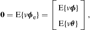
we conclude that ![]() is also orthogonal to
is also orthogonal to ![]() , so
, so
![]()
Assuming that ![]() is nonsingular, solving the normal Eq. (12.50) we obtain
is nonsingular, solving the normal Eq. (12.50) we obtain
![]() (12.62)
(12.62)
Now we have two interesting special cases: first, if ![]() and
and ![]() are orthogonal, i.e., if
are orthogonal, i.e., if ![]() , then
, then ![]() contains the first
contains the first ![]() elements of
elements of ![]() . Let us consider a specific example: assume that
. Let us consider a specific example: assume that
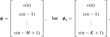 (12.63)
with ![]() . Then
. Then ![]() . This situation is very common in practice.
. This situation is very common in practice.
In this case, ![]() when
when ![]() is zero-mean white noise. This is one reason why white noise is the preferred input to be used in system identification: even in the (very likely in practice) case in which
is zero-mean white noise. This is one reason why white noise is the preferred input to be used in system identification: even in the (very likely in practice) case in which ![]() , at least the first elements of
, at least the first elements of ![]() are identified without bias.
are identified without bias.
On the other hand, if ![]() , then
, then ![]() is a mixture of the elements of
is a mixture of the elements of ![]() . This happens in (12.63) when the input sequence
. This happens in (12.63) when the input sequence ![]() is not white. In this case, the optimum filter
is not white. In this case, the optimum filter ![]() takes advantage of the correlation between the entries of
takes advantage of the correlation between the entries of ![]() and
and ![]() to estimate
to estimate ![]() given
given ![]() , and uses these estimated values to obtain a better approximation for
, and uses these estimated values to obtain a better approximation for ![]() . Sure enough, if you write down the problem of approximating
. Sure enough, if you write down the problem of approximating ![]() linearly from
linearly from ![]() , namely,
, namely,
![]()
you will see that the solution is exactly ![]() .
.
What is important to notice is that in both cases the optimum error ![]() is not equal to
is not equal to ![]() :
:
![]()
Partitioning ![]() , with
, with ![]() , we have
, we have
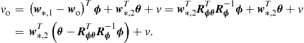
Although ![]() , you may check that indeed
, you may check that indeed ![]() .
.
As another example, assume that we have two variables such that ![]() , in which
, in which ![]() has zero mean and is independent of
has zero mean and is independent of ![]() , and
, and ![]() and
and ![]() are constants. Assume that we choose as regressor simply
are constants. Assume that we choose as regressor simply ![]() , so we try to solve
, so we try to solve
![]()
In this case we have
![]()
since ![]() . The optimum solution is thus
. The optimum solution is thus
![]()
and the optimum error is

However, ![]() is again orthogonal to
is again orthogonal to ![]() (but not to
(but not to ![]() , which we did not include in the regressor).
, which we did not include in the regressor).
What happens in the opposite situation, when we include more entries in ![]() than necessary? As one would expect, in this case the parameters related to these unnecessary entries will be zeroed in the optimum solution
than necessary? As one would expect, in this case the parameters related to these unnecessary entries will be zeroed in the optimum solution ![]() . This does not mean, however, that we should hasten to increase
. This does not mean, however, that we should hasten to increase ![]() to make
to make ![]() as large as possible, and leave to the filter the task of zeroing whatever was not necessary. This is because increasing the number of parameters to be estimated has a cost. The first and more obvious cost is in terms of memory and number of computations. However, we saw in Section 1.12.1.2 that an actual adaptive filter usually does not converge to the exact optimum solution, but rather hovers around it. Because of this, increasing the number of parameters may in fact decrease the quality of the solution. We explain this in more detail in Section 1.12.4.
as large as possible, and leave to the filter the task of zeroing whatever was not necessary. This is because increasing the number of parameters to be estimated has a cost. The first and more obvious cost is in terms of memory and number of computations. However, we saw in Section 1.12.1.2 that an actual adaptive filter usually does not converge to the exact optimum solution, but rather hovers around it. Because of this, increasing the number of parameters may in fact decrease the quality of the solution. We explain this in more detail in Section 1.12.4.
1.12.2.1.4 Zero and non-zero mean variables
Up to now we did not assume anything about the means of ![]() and
and ![]() . If both
. If both ![]() and
and ![]() have zero mean, we can interpret all autocorrelations as variances or covariance matrices, according to the case. To see this, assume that
have zero mean, we can interpret all autocorrelations as variances or covariance matrices, according to the case. To see this, assume that
![]() (12.64)
(12.64)
![]()
so the optimum error has zero mean. In this case, ![]() is the variance of
is the variance of ![]() , and
, and ![]() is the variance of
is the variance of ![]() , so (12.55) becomes
, so (12.55) becomes
![]() (12.65)
(12.65)
Since ![]() is positive-definite, we conclude that the uncertainty in
is positive-definite, we conclude that the uncertainty in ![]() (its variance) is never larger than the uncertainty in
(its variance) is never larger than the uncertainty in ![]() (Box 3).
(Box 3).
However, ![]() may have a nonzero mean if either
may have a nonzero mean if either ![]() or
or ![]() has nonzero mean. This is verified as follows. Define
has nonzero mean. This is verified as follows. Define
![]() (12.66)
(12.66)
then
![]()
in general (for example, if ![]() , but
, but ![]() ).
).
In many applications, ![]() should approximate some signal that is constrained to have zero mean, such as speech or noise, or because
should approximate some signal that is constrained to have zero mean, such as speech or noise, or because ![]() will be passed through a system with a high DC gain (such as an integrator), so it may be useful to guarantee that
will be passed through a system with a high DC gain (such as an integrator), so it may be useful to guarantee that ![]() has zero mean. How can this be done if the means of
has zero mean. How can this be done if the means of ![]() and
and ![]() are not zero? This problem is quite common, particularly when
are not zero? This problem is quite common, particularly when ![]() includes nonlinear functions of
includes nonlinear functions of ![]() . Fortunately, there are two easy solutions: First, if one knew the means of
. Fortunately, there are two easy solutions: First, if one knew the means of ![]() and
and ![]() , one could define zero-mean variables
, one could define zero-mean variables
![]() (12.67)
(12.67)
and use them instead of the original variables in (12.47). This is the simplest solution, but we often do not know the means ![]() and
and ![]() .
.
The second solution is used when the means are not known: simply add an extra term to ![]() , defining an extended regressor (not to be confused with the extended regressor from Section 1.12.2.1.3)
, defining an extended regressor (not to be confused with the extended regressor from Section 1.12.2.1.3)
 (12.68)
and an extended weight vector ![]() . The first coefficient of
. The first coefficient of ![]() will take care of the means, as we show next. The extended cross-correlation vector and autocorrelation matrix are
will take care of the means, as we show next. The extended cross-correlation vector and autocorrelation matrix are
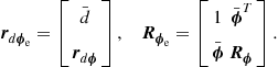
Assuming that ![]() and
and ![]() are nonsingular, we can compute
are nonsingular, we can compute ![]() if we evaluate the inverse of
if we evaluate the inverse of ![]() using Schur complements (See Fact 3 in Box 3), as follows
using Schur complements (See Fact 3 in Box 3), as follows
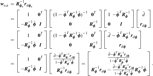
Using this result, we can evaluate now ![]() as follows (we used the fact that the inverse of a symmetric matrix is also symmetric from Box 3):
as follows (we used the fact that the inverse of a symmetric matrix is also symmetric from Box 3):

1.12.2.1.5 Sufficiently rich signals
We saw in Section 1.12.2.1.2 that even when ![]() is singular, we can recover the optimum
is singular, we can recover the optimum ![]() (with probability one), but not the optimum
(with probability one), but not the optimum ![]() . Let us study this problem in more detail, since it is important for system identification. So, what does it mean in practice to have a singular autocorrelation function
. Let us study this problem in more detail, since it is important for system identification. So, what does it mean in practice to have a singular autocorrelation function ![]() ? The answer to this question can be quite complicated when the input signals are nonstationary (i.e., when
? The answer to this question can be quite complicated when the input signals are nonstationary (i.e., when ![]() is not constant), so in this case we refer the interested reader to texts in adaptive control (such as [18]), which treat this problem in detail (although usually from a deterministic point of view). We consider here only the case in which the signals
is not constant), so in this case we refer the interested reader to texts in adaptive control (such as [18]), which treat this problem in detail (although usually from a deterministic point of view). We consider here only the case in which the signals ![]() are jointly wide-sense stationary.
are jointly wide-sense stationary.
In this case, ![]() may be singular because some entries of
may be singular because some entries of ![]() are linear combinations of the others. For example, if we choose
are linear combinations of the others. For example, if we choose ![]() and
and ![]() , then
, then
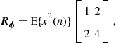
which is singular.
However, there are more subtle ways in which ![]() may become singular. Assume for example that our input sequence is given by
may become singular. Assume for example that our input sequence is given by
![]() (12.69)
(12.69)
where ![]() is the frequency, and
is the frequency, and ![]() is a random phase, uniformly distributed in the interval
is a random phase, uniformly distributed in the interval ![]() . This kind of model (sinusoidal signals with random phases), by the way, is the bridge between the periodic signals from Section 1.12.1.2 and the stochastic models discussed in this section. In this case, consider a vector
. This kind of model (sinusoidal signals with random phases), by the way, is the bridge between the periodic signals from Section 1.12.1.2 and the stochastic models discussed in this section. In this case, consider a vector ![]() formed from a delay line with
formed from a delay line with ![]() as input,
as input,
![]()
If ![]() , we have
, we have

The determinant of ![]() is
is ![]() if
if ![]() .
.
However, for any ![]() , the resulting
, the resulting ![]() will be singular: we can write
will be singular: we can write
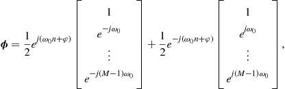
and since ![]() , we have
, we have
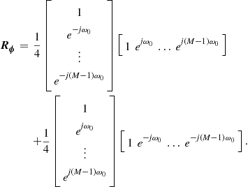
Since ![]() is the sum of two rank-one matrices, its rank is at most two. It will be two when
is the sum of two rank-one matrices, its rank is at most two. It will be two when ![]() , since in this case the vectors are linearly independent. We conclude that when the input signal is a sinusoid as in (12.69), the optimum solution to (12.47) will never be able to identify more than two coefficients. This argument can be generalized: if
, since in this case the vectors are linearly independent. We conclude that when the input signal is a sinusoid as in (12.69), the optimum solution to (12.47) will never be able to identify more than two coefficients. This argument can be generalized: if ![]() is composed of
is composed of ![]() sinusoids of different frequencies, then
sinusoids of different frequencies, then ![]() will be nonsingular if and only if
will be nonsingular if and only if ![]() .
.
The general conclusion is that ![]() will be singular or not, depending on which functions are chosen as inputs, and on the input signal. We say that the input is sufficiently rich for a given problem if it is such that
will be singular or not, depending on which functions are chosen as inputs, and on the input signal. We say that the input is sufficiently rich for a given problem if it is such that ![]() is nonsingular. We show a few examples next.
is nonsingular. We show a few examples next.
1.12.2.1.6 Examples
The concepts we saw in Sections 1.12.2.1.2–1.12.2.1.5 can be understood intuitively if we return to our example in Section 1.12.1.2. In that example, the true echo was obtained by filtering the input ![]() by an unknown
by an unknown ![]() , so we had
, so we had
where ![]() is the true order of the echo path,
is the true order of the echo path, ![]() and
and ![]() . We considered only one harmonic for simplicity.
. We considered only one harmonic for simplicity.
We are trying to cancel the echo, by constructing an approximated transfer function ![]() , which is modeled as an FIR filter with
, which is modeled as an FIR filter with ![]() coefficients. As we saw in Section 1.12.1.2, if
coefficients. As we saw in Section 1.12.1.2, if ![]() is a simple sinusoid, the echo will be completely canceled if we satisfy (12.8), reproduced below
is a simple sinusoid, the echo will be completely canceled if we satisfy (12.8), reproduced below
![]()
If ![]() , so
, so ![]() and
and ![]() , this condition becomes
, this condition becomes
![]()
with a single solution ![]() .
.
On the other hand, if the input were as before (a single sinusoid), but ![]() , so
, so ![]() , the equations would be
, the equations would be
![]()
and the solution would be unique (since ![]() is nonsingular), but would not approximate
is nonsingular), but would not approximate ![]() and
and ![]() in general.
in general.
This is an example of an undermodeled system, as we saw in Section 1.12.2.1.3. Figure 12.20 shows the LMS algorithm derived in Section 1.12.1.2 applied to this problem. Note that, even though ![]() do not converge to
do not converge to ![]() , in this example the error
, in this example the error ![]() does approximate well
does approximate well ![]() . This happens because in this case
. This happens because in this case ![]() is periodic, and the term
is periodic, and the term ![]() can be obtained exactly as a linear combination of
can be obtained exactly as a linear combination of ![]() and
and ![]() (Check that using the expressions for
(Check that using the expressions for ![]() from Section 1.12.2.1.3, we obtain
from Section 1.12.2.1.3, we obtain ![]() in this case.)
in this case.)
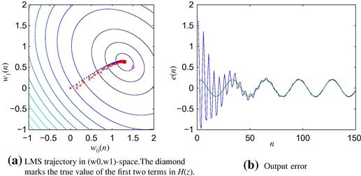
If we tried to identify ![]() by adding an extra coefficient to
by adding an extra coefficient to ![]() , the equations would be
, the equations would be
![]() (12.70)
(12.70)
Now ![]() , and
, and ![]() is a solution, but not the only one. Depending on the initial condition, the filter would converge to a different solution, as can be seen in Figure 12.21 (the level sets are not shown, because they are not closed curves in this case). The input is not rich enough (in harmonics) to excite the unknown system
is a solution, but not the only one. Depending on the initial condition, the filter would converge to a different solution, as can be seen in Figure 12.21 (the level sets are not shown, because they are not closed curves in this case). The input is not rich enough (in harmonics) to excite the unknown system ![]() so that the adaptive filter might identify it, as we saw in Section 1.12.2.1.5. However, for all solutions the error converges to
so that the adaptive filter might identify it, as we saw in Section 1.12.2.1.5. However, for all solutions the error converges to ![]() .
.

If the input had a second harmonic ![]() , we would add two more equations to (12.70), corresponding to
, we would add two more equations to (12.70), corresponding to ![]() , and the filter would be able to identify systems with up to four coefficients.
, and the filter would be able to identify systems with up to four coefficients.
The important message is that the adaptive filter only “sees” the error ![]() . If a mismatch between the true echo path
. If a mismatch between the true echo path ![]() and the estimated one
and the estimated one ![]() is not observable through looking only at the error signal, the filter will not converge to
is not observable through looking only at the error signal, the filter will not converge to ![]() . Whether a mismatch is observable or not through the error depends on both
. Whether a mismatch is observable or not through the error depends on both ![]() and the input signal being used: the input must excite a large enough number of frequencies so that
and the input signal being used: the input must excite a large enough number of frequencies so that ![]() can be estimated correctly. For this reason, in system identification a good input would be white noise.
can be estimated correctly. For this reason, in system identification a good input would be white noise.
1.12.2.2 Complex variables and multi-channel filtering
Adaptive filters used in important applications such as communications and radar have complex variables as input signals. In this section, we extend the results of Section 1.12.2.1 to consider complex signals. We start with the general solution, then restrict the result to the more usual case of circular signals.
We first show that the general solution for complex signals is equivalent to an adaptive filter with two inputs and two outputs: Indeed, if all input variables are complex, then the error ![]() will also be complex, that is,
will also be complex, that is, ![]() , where
, where ![]() are the real and imaginary parts of
are the real and imaginary parts of ![]() . We must then minimize
. We must then minimize ![]() , the total power of the complex signal
, the total power of the complex signal ![]() . The quadratic cost function (12.45) must be changed to
. The quadratic cost function (12.45) must be changed to
![]()
where ![]() is the complex conjugate of
is the complex conjugate of ![]() . Now, we need to be careful about what exactly is the coefficient vector
. Now, we need to be careful about what exactly is the coefficient vector ![]() in this case: If the regressor is
in this case: If the regressor is ![]() and
and ![]() , in principle
, in principle ![]() should be such that both its real and imaginary parts depend on both the real and imaginary parts of
should be such that both its real and imaginary parts depend on both the real and imaginary parts of ![]() , that is,
, that is,
![]() (12.71)
(12.71)
Note that there is no a priori reason for us to imagine that there should be a special relation between the pairs ![]() and
and ![]() . That is, we are dealing with two different coefficient vectors and one extended regressor:
. That is, we are dealing with two different coefficient vectors and one extended regressor:
 (12.72)
Let us proceed for the time being separating the real and imaginary channels of our filter. Later, in Section 1.12.2.2.1, we return to complex algebra. With these definitions, we can write
![]() (12.73)
(12.73)
The cost function then becomes
 (12.74)
where the autocorrelation matrix and cross-correlation vectors are given by
 (12.75)
where we simplified the notation, writing ![]() instead of
instead of ![]() instead of
instead of ![]() instead of
instead of ![]() , and so on.
, and so on.
Differentiating (12.74) to find the minimum, we obtain
![]() (12.76)
(12.76)
Therefore, the optimum filters satisfy
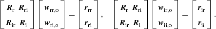 (12.77)
The optimum error is then
![]() (12.78)
(12.78)
There is also an orthogonality condition for this case: using (12.77), we obtain
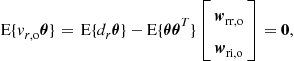 (12.79a)
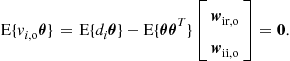 (12.79b)
The value of the cost function at the minimum can be obtained using this result. As in the case of real variables,
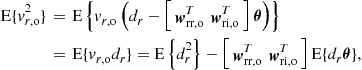
where we used (12.79a) in the second equality. Doing similarly for ![]() , we obtain
, we obtain
![]() (12.80a)
(12.80a)
![]() (12.80b)
(12.80b)
![]() (12.80c)
(12.80c)
What we have just described is a two-input/two-output optimal filter. In the next section, we re-derive it using complex algebra. Note that multi-channel filters have applications that are unrelated to complex variables, particularly in control [18], stereo echo cancellation [19,20], and active noise control [21–24].
1.12.2.2.1 Widely-linear complex least-mean squares
This general solution can be obtained in a more straightforward way if we use the complex gradients described in Box 6. Keeping the regressor ![]() as in (12.72) and defining the extended complex weight vector as
as in (12.72) and defining the extended complex weight vector as ![]() , we can write the cost function as
, we can write the cost function as
![]()
where we defined ![]() and
and ![]() . Note that
. Note that ![]() represents the Hermitian transpose, that is, transpose followed by conjugation. Differentiating
represents the Hermitian transpose, that is, transpose followed by conjugation. Differentiating ![]() with respect to
with respect to ![]() , as described in Box 6, we obtain
, as described in Box 6, we obtain
![]() (12.81)
(12.81)
The normal equations then become
![]() (12.82)
(12.82)
Expanding the real and imaginary parts of (12.82), we recover (12.77). Similarly, the optimum error and the minimum value of the cost are
![]() (12.83)
(12.83)
Comparing with (12.80), we see that ![]() , and the value of
, and the value of ![]() is the same as before. However, as you noticed, using a complex weight vector
is the same as before. However, as you noticed, using a complex weight vector ![]() and the complex derivatives of Box 6, all expressions are much simpler to derive.
and the complex derivatives of Box 6, all expressions are much simpler to derive.
The filter using a complex weight vector ![]() and the real regressor
and the real regressor ![]() constitutes a version of what is known as widely-linear complex filter. This version was recently proposed in [25] as a reduced-complexity alternative to the widely-linear complex filter originally proposed in [26,27], which uses as regressor the extended vector
constitutes a version of what is known as widely-linear complex filter. This version was recently proposed in [25] as a reduced-complexity alternative to the widely-linear complex filter originally proposed in [26,27], which uses as regressor the extended vector
 (12.84)
composed of the original regressor ![]() and its complex conjugate
and its complex conjugate ![]() (computational complexity is reduced because the number of operations required to compute
(computational complexity is reduced because the number of operations required to compute ![]() is about half of what is necessary to evaluate
is about half of what is necessary to evaluate ![]() ). Widely-linear estimation has been receiving much attention lately, due to new applications that have appeared [28–31].
). Widely-linear estimation has been receiving much attention lately, due to new applications that have appeared [28–31].
But why the name widely linear? The reason for this name is that the complex regressor ![]() does not appear linearly in the expressions, but only by separating its real and imaginary parts (as in
does not appear linearly in the expressions, but only by separating its real and imaginary parts (as in ![]() ) or by including its complex conjugate (as in
) or by including its complex conjugate (as in ![]() ). Both these expressions, from the point of view of a complex variable, are nonlinear.
). Both these expressions, from the point of view of a complex variable, are nonlinear.
What would be a linear complex filter, then? This is the subject of the next section.
1.12.2.2.2 Linear complex least-mean squares
There are many applications in which the data and regressor are such that their real and imaginary parts are similarly distributed, so that
![]() (12.85)
(12.85)
Under these conditions, we say that the pair ![]() is complex circular, or simply circular.
is complex circular, or simply circular.
In this case, we can rewrite (12.77) as

Expand these equations as follows (notice the change in order in (12.86b))
![]() (12.86a)
(12.86a)
![]() (12.86b)
(12.86b)
Now we can see that, if ![]() is a solution to (12.86a), then
is a solution to (12.86a), then
![]() (12.87)
(12.87)
is a solution to (12.86b). Therefore, when the input signals are circular, the number of degrees of freedom in the problem is actually smaller. In this case, there is a very nice way of recovering the solutions, working only with complex algebra. Indeed, defining ![]() , we have
, we have
 (12.88)
which is equivalent to (12.71) with the identities (12.87). Using this definition, it is possible to obtain the optimum solution (12.86a), (12.86b), and (12.87) using only complex algebra, following exactly the same steps as our derivation for the real case in the previous section.
This path is very useful, we can derive almost all results for real or complex circular adaptive filters using the same arguments. Let us see how it goes. First, define ![]() , so our problem becomes
, so our problem becomes
![]() (12.89)
(12.89)
Expanding the cost, recalling that now ![]() , we obtain
, we obtain
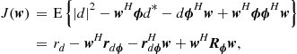 (12.90)
where we defined ![]() .
.
We need to find the minimum of this cost.One easy solution is to use the rules for differentiation of real functions of complex variables, as described in Box 6. These rules are very useful, and surprisingly easy to use: basically, we can treat ![]() and its conjugate
and its conjugate ![]() as if they were independent variables, that is
as if they were independent variables, that is
![]() (12.91)
(12.91)
Equating the gradient to zero, the solution is (assuming that ![]() is nonsingular)
is nonsingular)
![]() (12.92)
(12.92)
which is exactly equal to (12.51). This is the advantage of this approach: the expressions for complex and real problems are almost equal. The important differences are the conjugates that appear in the definitions of ![]() and
and ![]() , and the absence of a factor of
, and the absence of a factor of ![]() in the gradient (12.91). This follows from the definition of complex derivative we used (see Box 6). Here this difference is canceled out in the solution (12.92), but further on we will find situations in which there will be a different factor for the case of real and for the case of complex variables.
in the gradient (12.91). This follows from the definition of complex derivative we used (see Box 6). Here this difference is canceled out in the solution (12.92), but further on we will find situations in which there will be a different factor for the case of real and for the case of complex variables.
Let us check that (12.92) is really equivalent to (12.86a). Expanding ![]() and
and ![]() and using the circularity conditions (12.85), we obtain
and using the circularity conditions (12.85), we obtain
![]() (12.93a)
(12.93a)
![]() (12.93b)
(12.93b)
and
![]() (12.94)
(12.94)
so, equating the gradient (12.91) to zero, ![]() must satisfy
must satisfy
![]() (12.95)
(12.95)
Comparing the real and imaginary parts of (12.95) with (12.86a), we see that they indeed correspond to the same set of equations.
A few important remarks:
Remark 5
The orthogonality condition still holds in the complex circular case, but with a small difference: defining the optimum error as before,
![]()
we obtain, noting that ![]() ,
,
![]() (12.96)
(12.96)
Remark 7
The optimum error power can be obtained as in the real case, and is equal to
![]() (12.97)
(12.97)
Box 4:
Least mean-squares estimation
Here we consider the general problem of finding the optimum relation ![]() between
between ![]() and
and ![]() , such that
, such that
![]() (12.98)
(12.98)
without restricting ![]() to a particular class.
to a particular class.
In order to understand well this problem, let us consider first the simpler case where the relation between ![]() and
and ![]() is memoryless, that is, our function depends only on the current value of
is memoryless, that is, our function depends only on the current value of ![]() . Dropping the time index to simplify the notation, our problem then becomes how to find a function
. Dropping the time index to simplify the notation, our problem then becomes how to find a function ![]() that, applied to a certain random variable
that, applied to a certain random variable ![]() , approximates a certain random variable
, approximates a certain random variable ![]() so that the mean-square error is minimized, that is, we want to solve
so that the mean-square error is minimized, that is, we want to solve
![]() (12.99)
(12.99)
Assume that the joint probability density function ![]() of
of ![]() and
and ![]() is known (we are assuming that
is known (we are assuming that ![]() and
and ![]() are continuous random variables, but the final result in (12.100) also holds if they are discrete). Then,
are continuous random variables, but the final result in (12.100) also holds if they are discrete). Then,
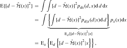 (12.100)
where we use the subscripts ![]() and
and ![]() to highlight that the expectations are taken with respect to
to highlight that the expectations are taken with respect to ![]() or
or ![]() only.
only.
Note that the inner integrand ![]() in (12.100) is nonnegative. Therefore, if we minimize it for each value of
in (12.100) is nonnegative. Therefore, if we minimize it for each value of ![]() , we will obtain the minimum of the full expression. That is, the optimum
, we will obtain the minimum of the full expression. That is, the optimum ![]() is the function defined by
is the function defined by
![]() (12.101)
(12.101)
It is important to remember that, fixed ![]() is simply a number. This can be seen more easily expanding the expectations in (12.101)
is simply a number. This can be seen more easily expanding the expectations in (12.101)

Differentiating with respect to ![]() and equating to zero, we obtain the solution
and equating to zero, we obtain the solution
![]() (12.102)
(12.102)
which is indeed a function of ![]() , as desired.
, as desired.
Let us study the properties of this solution. First, define
![]()
Note that ![]() and
and ![]() are not necessarily equal to
are not necessarily equal to ![]() and
and ![]() from (12.40). Evaluating the average of
from (12.40). Evaluating the average of ![]() , we obtain
, we obtain
![]()
by an argument similar to that used to obtain (12.100). We conclude that ![]() has zero mean. In addition, for any function
has zero mean. In addition, for any function ![]() of
of ![]() for which the expected values exist, we have
for which the expected values exist, we have
![]() (12.103)
(12.103)
since ![]() . This result means that the error
. This result means that the error ![]() is uncorrelated to any function of the reference data
is uncorrelated to any function of the reference data ![]() , which is a very strong condition. It basically means that we have extracted all second-order information available in
, which is a very strong condition. It basically means that we have extracted all second-order information available in ![]() about
about ![]() .
.
We remark that (12.103) does not imply that ![]() and
and ![]() are independent. A simple counter-example is the following: consider two discrete-valued random variables
are independent. A simple counter-example is the following: consider two discrete-valued random variables ![]() and
and ![]() with joint probabilities given by Table 12.1. Then
with joint probabilities given by Table 12.1. Then ![]() , but
, but ![]() and
and ![]() are not independent.
are not independent.

In the more general case in which ![]() is allowed to depend on previous samples of
is allowed to depend on previous samples of ![]() , the arguments and the final conclusion are similar:
, the arguments and the final conclusion are similar:
![]() (12.104)
(12.104)
and defining
![]()
it holds that ![]() has zero mean and is uncorrelated with any function of
has zero mean and is uncorrelated with any function of ![]() :
:
![]() (12.105)
(12.105)
Note that, in general, the optimal solution of (12.104) depends on ![]() , so we should write
, so we should write
![]() (12.106)
(12.106)
to make the time dependence explicit.
We can now return to the question at the start of this section: From our results thus far, we see that minimizing ![]() leads to a model which relates
leads to a model which relates ![]() and the sequence
and the sequence ![]() such that
such that
![]()
in which ![]() is uncorrelated with any function
is uncorrelated with any function ![]() of
of ![]() In other words, the solution of (12.104) imposes such a model on our data, even if this model makes no physical sense at all. This is an important point: such a model will always result from the minimization of the mean-square error, at least as long as the statistics of
In other words, the solution of (12.104) imposes such a model on our data, even if this model makes no physical sense at all. This is an important point: such a model will always result from the minimization of the mean-square error, at least as long as the statistics of ![]() and
and ![]() are such that the expected values in (12.104) are finite.
are such that the expected values in (12.104) are finite.
Now, what if we knew beforehand, by physical arguments about the data, that a model such as (12.40) holds between ![]() and
and ![]() , such that
, such that ![]() has zero mean and is uncorrelated to any function of
has zero mean and is uncorrelated to any function of ![]() ? Will it result that the solution of (12.104) will be such that
? Will it result that the solution of (12.104) will be such that
![]()
To answer this question, let us go back to (12.99), and use (12.40) to find the solution. We thus have (we omit the arguments of ![]() and
and ![]() for simplicity)
for simplicity)
![]()
Since ![]() is orthogonal to any function of
is orthogonal to any function of ![]() by assumption, it will be orthogonal to
by assumption, it will be orthogonal to ![]() and
and ![]() in particular. Therefore, we can simplify the cost as
in particular. Therefore, we can simplify the cost as
![]() (12.107)
(12.107)
Both terms in (12.107) are positive, and only the first depends on ![]() . Therefore, the solution is indeed
. Therefore, the solution is indeed ![]() and
and ![]() , as one would wish (to be precise,
, as one would wish (to be precise, ![]() and
and ![]() could differ on a set of probability zero).
could differ on a set of probability zero).
We conclude that we can use (12.102) as a criterion for separating the two parts ![]() and
and ![]() of our model for
of our model for ![]() if and only if
if and only if ![]() satisfies (12.105). This holds, for example, if
satisfies (12.105). This holds, for example, if ![]() has zero mean and is independent of
has zero mean and is independent of ![]() for all
for all ![]() .
.
Note that since ![]() is itself a function of
is itself a function of ![]() , (12.105) implies that
, (12.105) implies that
![]()
and we have

Recalling that ![]() , if we add and subtract
, if we add and subtract ![]() to the last result, we conclude that
to the last result, we conclude that
![]() (12.108)
(12.108)
where ![]() and
and ![]() are the variances of
are the variances of ![]() and of
and of ![]() .
.
The solution we just found is very general (it assumes little about ![]() ), and there are ways of computing it adaptively from the data, using for example algorithms known as particle filters [32]. The solution requires, however, that one builds approximations for the joint probability distribution of
), and there are ways of computing it adaptively from the data, using for example algorithms known as particle filters [32]. The solution requires, however, that one builds approximations for the joint probability distribution of ![]() and
and ![]() , which in general requires a large amount of data, resulting in relatively high complexity and relatively slow convergence. If you know more about the relation between
, which in general requires a large amount of data, resulting in relatively high complexity and relatively slow convergence. If you know more about the relation between ![]() and
and ![]() , this information might be used to constrain the search to a smaller class of problems, potentially leading to simpler algorithms with faster convergence. That is the goal of adaptive filters, and the reason why we restricted ourselves to this case in the main text.
, this information might be used to constrain the search to a smaller class of problems, potentially leading to simpler algorithms with faster convergence. That is the goal of adaptive filters, and the reason why we restricted ourselves to this case in the main text.
Box 5:
Convex functions
Convex sets are such that lines between any two points in the set always stay entirely in the set (see Figure 12.22). More formally, a set ![]() is convex if
is convex if
![]()
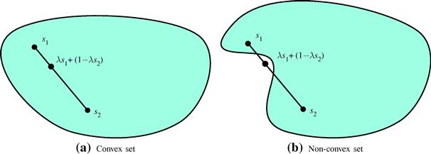
Convex functions, on the other hand, are functions ![]() such that for all
such that for all ![]() and
and ![]() ,
,
![]()
The function is called strictly convex if the inequality is strict (< instead of ![]() ). For example,
). For example, ![]() is strictly convex. Figure 12.23 shows examples of convex and non-convex functions. An important property of strictly convex functions is that they always have a unique minimum, that is, they never have sub-optimal local minima.
is strictly convex. Figure 12.23 shows examples of convex and non-convex functions. An important property of strictly convex functions is that they always have a unique minimum, that is, they never have sub-optimal local minima.
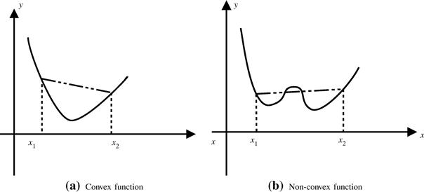
Box 6:
Wirtinger derivatives and minima of functions of a complex variable
Suppose you want to minimize a function
![]() (12.109)
(12.109)
that is, a function that takes a complex argument to a real value. The minimization problem is well defined, since the image of ![]() is real. However, we cannot use standard arguments about derivatives and stationary points to find the minimum, because a function like this is never analytic, that is, the standard derivative used in complex analysis does not exist.
is real. However, we cannot use standard arguments about derivatives and stationary points to find the minimum, because a function like this is never analytic, that is, the standard derivative used in complex analysis does not exist.
To see why, we need to think about ![]() as a function of two variables,
as a function of two variables, ![]() and
and ![]() , the real and imaginary parts of
, the real and imaginary parts of ![]() . Take
. Take ![]() for example. We can write it as a function of
for example. We can write it as a function of ![]() and
and ![]() as
as
![]() (12.110)
(12.110)
Since it is a function of two variables, the derivatives in principle depend on the direction we are moving along. Consider the derivative at a point ![]() along the
along the ![]() axis, that is, keeping
axis, that is, keeping ![]() constant:
constant:
![]()
On the other hand, along the ![]() axis, we have
axis, we have
![]()
that is, the derivative at point ![]() is different according to the direction we are moving. This is essentially what is meant by saying that the function is not analytic at
is different according to the direction we are moving. This is essentially what is meant by saying that the function is not analytic at ![]() .
.
For contrast, consider now the analytic function ![]() . Its derivative is the same, no matter which direction we take:
. Its derivative is the same, no matter which direction we take:
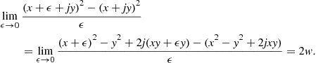
Similarly, differentiating along the ![]() axis we obtain again the same result
axis we obtain again the same result
![]()
When the derivative at a certain point ![]() is the same along every direction, we can define derivatives of complex functions writing simply
is the same along every direction, we can define derivatives of complex functions writing simply
![]() (12.111)
(12.111)
since we know the limit does not depend on the direction along which ![]() goes to zero.
goes to zero.
It can be shown that a function is analytic at a given point only if the Cauchy-Riemann conditions hold at that point. Separating a generic complex function ![]() into its real and imaginary parts
into its real and imaginary parts ![]() , the Cauchy-Riemann conditions are [33]
, the Cauchy-Riemann conditions are [33]
![]()
In the case of a real function of a complex variable, such as ![]() defined as in (12.109),
defined as in (12.109), ![]() , and of course the conditions could hold only for points in which the real part has zero partial derivatives.
, and of course the conditions could hold only for points in which the real part has zero partial derivatives.
This means that we cannot search for the stationary points of a function such as (12.109) using the derivative defined as in (12.111). We could of course always go back and interpret the function as a function of two variables, as we did in (12.110). In order to find the minimum of ![]() , we would need to find the stationary points of
, we would need to find the stationary points of ![]()
![]()
This works just fine, of course, but there is a nice trick, which allows us to keep working with complex variables in a simple way. The idea is to define derivatives differently, such that optimization problems become easy to solve, using what is known as Wirtinger calculus.
Real functions of complex variables are usually defined in terms of variables and its conjugates, since ![]() and
and ![]() are both real. The idea is to define derivatives such that
are both real. The idea is to define derivatives such that ![]() and
and ![]() can be treated as if they were independent variables, as follows. Despite the motivation, the new derivatives are defined for general functions
can be treated as if they were independent variables, as follows. Despite the motivation, the new derivatives are defined for general functions ![]() .
.
Define partial derivatives of a function ![]() with respect to
with respect to ![]() and
and ![]() as
as
![]() (12.112)
(12.112)
You can check that if ![]() is analytic at a given point (so
is analytic at a given point (so ![]() satisfies the Cauchy-Riemann conditions at that point), then
satisfies the Cauchy-Riemann conditions at that point), then ![]() at that point.
at that point.
Consider, for example, ![]() . Then,
. Then,
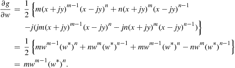
As advertised, the final result is what we would obtain if we had treated ![]() and
and ![]() as two independent variables. Similarly, you can check that
as two independent variables. Similarly, you can check that
![]()
An important special case is the quadratic function ![]() , which assumes only real values if
, which assumes only real values if ![]() and
and ![]() are real. Using the previous result, we see that
are real. Using the previous result, we see that
![]()
Note that there is no factor of ![]() in this case. This difference between Wirtinger derivatives and standard real derivatives will propagate to many expressions in this text.
in this case. This difference between Wirtinger derivatives and standard real derivatives will propagate to many expressions in this text.
Now, the definitions (12.112) are useful for minimizing real functions of complex variables as in (12.109), since from (12.112)
![]()
Applying this idea to our quadratic function, we see that
![]()
if ![]() . In addition,
. In addition,
![]()
and we can conclude that ![]() is a minimum as long as
is a minimum as long as ![]() .
.
The same conclusions could easily be obtained working directly with ![]() . The Wirtinger derivatives are merely a shortcut, that makes working with complex variables very similar to working with real variables. A good detailed description of Wirtinger derivatives can be found in [34].
. The Wirtinger derivatives are merely a shortcut, that makes working with complex variables very similar to working with real variables. A good detailed description of Wirtinger derivatives can be found in [34].
In the vector case, the definitions and results are very similar. Given a function
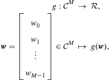
with ![]() ,
, ![]() , we define
, we define

Using our definition of gradients, the second derivative of ![]() (its Hessian) is
(its Hessian) is
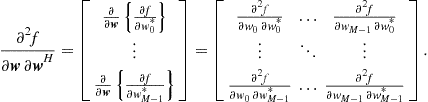
The most important example is the quadratic function
![]()
where ![]() is a real variable, and
is a real variable, and ![]() is Hermitian symmetric. Then, we have
is Hermitian symmetric. Then, we have
![]()
We see that a stationary point of ![]() is such that
is such that ![]() . In addition,
. In addition,
![]()
and we conclude that ![]() is the single point of minimum of
is the single point of minimum of ![]() if and only if
if and only if ![]() is positive-definite.
is positive-definite.
Note that in the complex case, the gradient and the Hessian do not have the factors of ![]() that we saw in the real case (see Box 1).
that we saw in the real case (see Box 1).
1.12.3 Stochastic algorithms
In this section, we focus on three of the most important adaptive algorithms: the least-mean squares (LMS) algorithm, the normalized least-mean squares (NLMS) algorithm, and the recursive least-squares (RLS) algorithm, which are the basis of many other algorithms. These three stochastic algorithms are derived in detail and analyzed using different methods. We present different approaches for analyzing an adaptive filter, because the variety and complexity of their behavior makes it difficult for a single technique to be able to handle all situations. The analyses provided here allow us to predict the behavior of the algorithms in transient and steady-state, and choose values of parameters (such as the step-size) for which the filters operate adequately. In particular, we study conditions under which the filters will remain stable.
We assume linearly parametrized classes, such as FIR ![]() and Volterra
and Volterra ![]() filters (see Section 1.12.2.1). In these classes, each element of the input regressor vector is given by a certain function
filters (see Section 1.12.2.1). In these classes, each element of the input regressor vector is given by a certain function ![]()
![]() of
of ![]() . In the case of length-
. In the case of length-![]() FIR filters, we have
FIR filters, we have
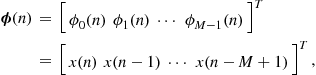 (12.113)
whereas in the case of second-order Volterra filters with memory ![]() and real-valued signals, we have
and real-valued signals, we have
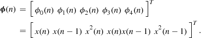 (12.114)
As much as possible, our presentation in this section is independent of the choices of ![]() and
and ![]() . However, some algorithms are designed for a specific class
. However, some algorithms are designed for a specific class ![]() (the most common case are fast algorithms designed for FIR filters (12.113)). In these cases, we will alert the reader of the restriction.
(the most common case are fast algorithms designed for FIR filters (12.113)). In these cases, we will alert the reader of the restriction.
Using the results of Box 6, the derivation of algorithms for real or circular complex inputs is very similar, the only differences being the need of conjugating a few variables in some expressions, and the appearance of a factor ![]() in the expressions of gradients of functions of real variables, and
in the expressions of gradients of functions of real variables, and ![]() in the complex case.
in the complex case.
In general, the output of a length-![]() adaptive filter is given by
adaptive filter is given by
![]() (12.115)
(12.115)
In the case of Volterra filters, it is common to use the notation ![]() for the weight related to the input
for the weight related to the input ![]() (see Eq. (12.43)). However, to obtain a common formulation independent of the class
(see Eq. (12.43)). However, to obtain a common formulation independent of the class ![]() , we denote the weight vector as
, we denote the weight vector as
![]() (12.116)
(12.116)
The task of the adaptive filter will be to choose in a recursive form the values of the parameters ![]() that best fit the data at each time instant
that best fit the data at each time instant ![]() .
.
Figure 12.24 shows the scheme of a length-![]() adaptive filter for linearly parametrized classes, where
adaptive filter for linearly parametrized classes, where ![]() denotes the set of functions
denotes the set of functions ![]() ,
, ![]() of
of ![]() that generate the elements
that generate the elements ![]() of the input regressor vector
of the input regressor vector ![]() . The number of samples of the signal
. The number of samples of the signal ![]() depends on the class
depends on the class ![]() and is given by
and is given by ![]() . An FIR filter with length
. An FIR filter with length ![]() requires
requires ![]() samples. On the other hand, a Volterra filter with memory
samples. On the other hand, a Volterra filter with memory ![]() , requires
, requires ![]() samples, but the length of the corresponding adaptive filter depends on the order of the Volterra series expansion. At each time instant, the output of the adaptive filter
samples, but the length of the corresponding adaptive filter depends on the order of the Volterra series expansion. At each time instant, the output of the adaptive filter ![]() is compared with the desired signal
is compared with the desired signal ![]() to compute the error
to compute the error ![]() . In order to minimize a cost function of this error, a stochastic algorithm uses
. In order to minimize a cost function of this error, a stochastic algorithm uses ![]() to adjust the filter weights.
to adjust the filter weights.

1.12.3.1 LMS algorithm
The update equation of the steepest-descent algorithm is given by
![]() (12.117)
(12.117)
where ![]() is a step-size and
is a step-size and ![]() (resp.,
(resp., ![]() ) for complex (resp., real) data (see Box 6). This algorithm requires exact measurements of the gradient vector. For the case of minimization of the mean-square error, that is, if
) for complex (resp., real) data (see Box 6). This algorithm requires exact measurements of the gradient vector. For the case of minimization of the mean-square error, that is, if ![]() ,
,
![]() (12.118)
(12.118)
at each iteration ![]() (see Box 1 for an introduction to gradient algorithms). Note that the exact gradient requires a prior knowledge of the correlation matrix
(see Box 1 for an introduction to gradient algorithms). Note that the exact gradient requires a prior knowledge of the correlation matrix ![]() and the cross-correlation vector
and the cross-correlation vector ![]() , which is not feasible in real-time applications. For example, in the hands-free telephone application described in Section 1.12.1.1, the input signal of the adaptive filter is the far-end speech (see Figures 12.3 and 12.4). A speech signal is nonstationary and therefore, it is not possible to obtain exact estimates for
, which is not feasible in real-time applications. For example, in the hands-free telephone application described in Section 1.12.1.1, the input signal of the adaptive filter is the far-end speech (see Figures 12.3 and 12.4). A speech signal is nonstationary and therefore, it is not possible to obtain exact estimates for ![]() and
and ![]() at each time instant. Furthermore, good estimates would demand much processing time, which could insert an inadmissible delay in the system, making this approach not feasible, except in off-line applications. Similar restrictions appear in virtually all adaptive filtering applications.
at each time instant. Furthermore, good estimates would demand much processing time, which could insert an inadmissible delay in the system, making this approach not feasible, except in off-line applications. Similar restrictions appear in virtually all adaptive filtering applications.
To circumvent this problem, a stochastic version of the steepest descent algorithm was proposed, the least-mean squares (LMS) algorithm. Instead of minimizing the exact mean-square error, the LMS algorithm minimizes a straightforward approximation to it: ![]() . The idea, as we saw in Section 1.12.1.2.4, is that the algorithm will approximately average the cost-function if adaptation is slow (small step-size). The estimation error is
. The idea, as we saw in Section 1.12.1.2.4, is that the algorithm will approximately average the cost-function if adaptation is slow (small step-size). The estimation error is
![]() (12.119)
(12.119)
so the gradient of the instantaneous cost function is
![]() (12.120)
(12.120)
Since ![]() depends on the old estimate of the weight vector, it is called an a priori estimation error, by opposition to the a posteriori error that will be introduced in (12.129). Instead of minimizing the instantaneous cost function, the stochastic gradient defined in (12.120) can be obtained by replacing the instantaneous estimates
depends on the old estimate of the weight vector, it is called an a priori estimation error, by opposition to the a posteriori error that will be introduced in (12.129). Instead of minimizing the instantaneous cost function, the stochastic gradient defined in (12.120) can be obtained by replacing the instantaneous estimates
![]() (12.121)
(12.121)
and
![]() (12.122)
(12.122)
in (12.118).
Replacing (12.120) in (12.117), we arrive at the update equation for LMS, i.e.,
![]() (12.123)
(12.123)
As explained in Section 1.12.1.2.4 and illustrated in the animations of Figure 12.9, although there is no explicit average being taken in the LMS algorithm, it in fact computes an implicit approximate average if the step-size is small.
The LMS algorithm is summarized in Table 12.2. Its computational cost increases linearly with the length of the filter, i.e., the computational cost is ![]() . Table 12.3 shows the number of real multiplications and real additions per iteration for real and complex-valued signals. The quantities inside brackets were computed in previous steps. We assume that a complex multiplication requires 4 real multiplications and 2 real additions (it is possible to use less multiplications and more additions), and a complex addition requires 2 real additions. Different ways of carrying out the calculations may result in a different computational cost. For example, if we first computed
. Table 12.3 shows the number of real multiplications and real additions per iteration for real and complex-valued signals. The quantities inside brackets were computed in previous steps. We assume that a complex multiplication requires 4 real multiplications and 2 real additions (it is possible to use less multiplications and more additions), and a complex addition requires 2 real additions. Different ways of carrying out the calculations may result in a different computational cost. For example, if we first computed ![]() followed by
followed by ![]() , LMS would require
, LMS would require ![]() more real multiplications per iteration than the ordering of Table 12.3, considering real-valued signals. For complex-valued signals, the cost would be even higher, since LMS would require
more real multiplications per iteration than the ordering of Table 12.3, considering real-valued signals. For complex-valued signals, the cost would be even higher, since LMS would require ![]() and
and ![]() more real multiplications and real additions, respectively.
more real multiplications and real additions, respectively.

Table 12.3
Computational Cost of the LMS Algorithm for Complex and Real-Valued Signals in Terms of Real Multiplications and Real Additions Per Iteration

1.12.3.1.1 A deterministic approach for the stability of LMS
Finding the range of step-sizes such that the recursion (12.123) converges is a complicated task. There are two main approaches to finding the maximum step-size: an average approach and a deterministic (worst-case) approach. The average approach will be treated in Section 1.12.4.3. Since the deterministic approach is easy to explain intuitively, we address it in the sequel (although a precise proof is not so simple, see [35,36] for a full analysis).
For simplicity, assume that our filter is such that ![]() . Although this is not a very likely situation to encounter in practice, it allows us to avoid technical details that would complicate considerably the discussion, and still arrive at the important conclusions.
. Although this is not a very likely situation to encounter in practice, it allows us to avoid technical details that would complicate considerably the discussion, and still arrive at the important conclusions.
Let us rewrite the LMS recursion, expanding the error with ![]() as
as ![]() to obtain
to obtain
![]() (12.124)
(12.124)
This is a linear system, but not a time-invariant one. It will be stable if the eigenvalues ![]() of the matrix
of the matrix ![]() satisfy
satisfy
![]() (12.125)
(12.125)
Be careful, if ![]() were not identically zero, condition (12.125) would have to be slightly modified to guarantee stability (see, e.g., [36,37]).
were not identically zero, condition (12.125) would have to be slightly modified to guarantee stability (see, e.g., [36,37]).
The eigenvalues of ![]() are easy to find, if we note that
are easy to find, if we note that ![]() is an eigenvector of
is an eigenvector of ![]() (the case
(the case ![]() is trivial):
is trivial):
![]()
where ![]() is the square of the Euclidean norm. The corresponding eigenvalue is
is the square of the Euclidean norm. The corresponding eigenvalue is ![]() . All other eigenvalues are equal to one (the eigenvectors are all vectors orthogonal to
. All other eigenvalues are equal to one (the eigenvectors are all vectors orthogonal to ![]() .) Therefore, the LMS algorithm (12.124) will be stable whenever
.) Therefore, the LMS algorithm (12.124) will be stable whenever
![]() (12.126)
(12.126)
The supremum (![]() ) of a sequence is an extension to the maximum, defined to avoid a technicality. Consider the sequence
) of a sequence is an extension to the maximum, defined to avoid a technicality. Consider the sequence ![]() . Strictly speaking, it has no maximum, since there is no
. Strictly speaking, it has no maximum, since there is no ![]() for which
for which ![]() for all
for all ![]() . The supremum is defined so we can avoid this problem:
. The supremum is defined so we can avoid this problem: ![]() . Therefore, the supremum is equal to the maximum whenever the later exists, but is also defined for some sequences that do not have a maximum. The infimum
. Therefore, the supremum is equal to the maximum whenever the later exists, but is also defined for some sequences that do not have a maximum. The infimum![]() has a similar relation to the minimum.
has a similar relation to the minimum.
This condition is sufficient for stability, but is too conservative, since ![]() is not at its highest value at all instants. A popular solution is to use normalization. The idea is simple: adopt a time-variant step-size
is not at its highest value at all instants. A popular solution is to use normalization. The idea is simple: adopt a time-variant step-size ![]() such that
such that
![]() (12.127)
(12.127)
with ![]() and where
and where ![]() is used to avoid division by zero. The resulting algorithm is known as normalized LMS (NLMS). We will talk more about it in the next section.
is used to avoid division by zero. The resulting algorithm is known as normalized LMS (NLMS). We will talk more about it in the next section.
1.12.3.2 Normalized LMS algorithm
One problem with the LMS algorithm is how to choose the step-size. How large should it be to enable a high convergence rate, provide an acceptable misadjustment, and even ensure the stability of LMS? More importantly, how can this choice be made so that the filter will work correctly even for very different input signals? One answer to this problem is the normalized LMS algorithm which we describe now. It uses a time varying step-size, which is particularly useful when the statistics of the input signals change quickly.
Thus, replacing the fixed step-size ![]() by a time varying step-size
by a time varying step-size ![]() in (12.123), we obtain
in (12.123), we obtain
![]() (12.128)
(12.128)
In order to increase the convergence speed, we could try to find ![]() such that the a posteriori estimation error,
such that the a posteriori estimation error,
![]() (12.129)
(12.129)
is zeroed. Note that, in contrast to the a priori estimation error defined in (12.119), ![]() depends on the updated estimate of the weight vector, hence the name a posteriori estimation error. Replacing (12.128) in (12.129), we obtain
depends on the updated estimate of the weight vector, hence the name a posteriori estimation error. Replacing (12.128) in (12.129), we obtain
 (12.130)
In order to enforce ![]() at each time instant
at each time instant ![]() , we must select
, we must select
![]() (12.131)
(12.131)
Replacing (12.131) in (12.128), we obtain the update equation of the normalized least-squares algorithm, i.e.,
![]() (12.132)
(12.132)
Note that the time varying step-size ![]() depends inversely on the instantaneous power of the input vector
depends inversely on the instantaneous power of the input vector ![]() . Indeed, we will show in Section 1.12.4.3 that the maximum value of the fixed step-size
. Indeed, we will show in Section 1.12.4.3 that the maximum value of the fixed step-size ![]() to ensure the convergence and mean-square stability of LMS depends inversely on the power of the input signal.
to ensure the convergence and mean-square stability of LMS depends inversely on the power of the input signal.
In order to make (12.132) more reliable for practical implementations, it is common to introduce two positive constants: a fixed step-size ![]() to control the rate of convergence (and the misadjustment) and the regularization factor
to control the rate of convergence (and the misadjustment) and the regularization factor ![]() to prevent division by a small value when
to prevent division by a small value when ![]() is small. With these constants, the NLMS update equation reduces to
is small. With these constants, the NLMS update equation reduces to
![]() (12.133)
(12.133)
Some authors refer to (12.132) as NLMS and to (12.133) as ![]() -NLMS. However, for simplicity we will refer to both as NLMS. The name “normalized” is due to a most useful property of NLMS: the range of values of
-NLMS. However, for simplicity we will refer to both as NLMS. The name “normalized” is due to a most useful property of NLMS: the range of values of ![]() for which the algorithm remains stable is independent of the statistics of
for which the algorithm remains stable is independent of the statistics of ![]() , i.e.,
, i.e., ![]() , as can be observed in Section 1.12.3.1.1.
, as can be observed in Section 1.12.3.1.1.
As pointed out in [3], the NLMS algorithm can also be interpreted as a quasi-Newton algorithm. As briefly explained in Box 1, a quasi-Newton algorithm updates the weights using approximations for the Hessian matrix and gradient vector, i.e.,
![]() (12.134)
(12.134)
Assuming the following instantaneous approximations
![]() (12.135)
(12.135)
and
![]() (12.136)
(12.136)
and replacing them in (12.134), we arrive at the stochastic recursion
![]() (12.137)
(12.137)
The term ![]() guarantees that (12.136) is invertible (a rank-one matrix such as
guarantees that (12.136) is invertible (a rank-one matrix such as ![]() is never invertible).
is never invertible).
To compute ![]() , we can use the matrix inversion lemma (Box 3), which gives us an expression for the inverse of an
, we can use the matrix inversion lemma (Box 3), which gives us an expression for the inverse of an ![]() matrix of the form
matrix of the form
![]() (12.138)
(12.138)
where ![]() and
and ![]() are two square matrices with dimensions
are two square matrices with dimensions ![]() and
and ![]() , respectively, and
, respectively, and ![]() is an
is an ![]() matrix. According to the matrix inversion lemma, the inverse of
matrix. According to the matrix inversion lemma, the inverse of ![]() is given by
is given by
![]() (12.139)
(12.139)
Thus, identifying
![]()
we obtain
![]() (12.140)
(12.140)
Multiplying (12.140) from the right by ![]() , after some algebraic manipulations, we get
, after some algebraic manipulations, we get
![]() (12.141)
(12.141)
Replacing (12.141) in (12.137), we arrive at (12.133). Since Newton-based algorithms converge faster than gradient-based algorithms, it is expected that NLMS exhibits a higher convergence rate than that of LMS, which is indeed the case in general.
The NLMS algorithm is summarized in Table 12.4. To obtain its computational cost, we can use the same procedure considered in the computation of the number of operations of LMS (see Table 12.3). For complex-valued signals, NLMS requires ![]() real multiplications,
real multiplications, ![]() real additions and one real division per iteration. For real-valued signals, it requires
real additions and one real division per iteration. For real-valued signals, it requires ![]() real multiplications and
real multiplications and ![]() real additions per iteration. Note that for input vectors with a shift structure such as the FIR filters of Eq. (12.113), its computational cost can be reduced if
real additions per iteration. Note that for input vectors with a shift structure such as the FIR filters of Eq. (12.113), its computational cost can be reduced if ![]() is computed by the following recursion
is computed by the following recursion
![]() (12.142)
(12.142)
with initialization ![]() .
.
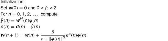
1.12.3.3 RLS algorithm
The convergence rate of LMS-type algorithms varies considerably with the input signal ![]() , since they are based on steepest-descent optimization algorithms. If
, since they are based on steepest-descent optimization algorithms. If ![]() is a white noise, the convergence rate is high. On the other hand, if the correlation between successive samples of
is a white noise, the convergence rate is high. On the other hand, if the correlation between successive samples of ![]() is high, LMS-type algorithms converge slowly. The RLS algorithm does not have this drawback. However, this advantage has a price: a considerable increase in the computational cost. Furthermore, numerical errors play a more important role in RLS and may even lead to divergence of the weight estimates. Different versions of RLS were proposed to circumvent this problem. In the sequel, we obtain the equations of the conventional RLS algorithm.
is high, LMS-type algorithms converge slowly. The RLS algorithm does not have this drawback. However, this advantage has a price: a considerable increase in the computational cost. Furthermore, numerical errors play a more important role in RLS and may even lead to divergence of the weight estimates. Different versions of RLS were proposed to circumvent this problem. In the sequel, we obtain the equations of the conventional RLS algorithm.
The RLS can be derived in different ways (much as NLMS). Each form of arriving at the algorithm highlights a different set of its properties: one that leads to many new algorithms and insights is the connection between RLS and Kalman filters described in [38].
We present here shorter routes, starting with a derivation based on deterministic arguments. In fact, RLS solves a deterministic least-squares problem, which is based on the weighted least-squares cost function
![]() (12.143)
(12.143)
where ![]() is a constant known as forgetting factor,
is a constant known as forgetting factor,
![]() (12.144)
(12.144)
are a posteriori errors and
![]() (12.145)
(12.145)
The factor ![]() emphasizes the most recent errors, forgetting the errors from the remote past. This is important, otherwise the algorithm would give too much weight to the remote past and would not be able to track variations in the input signals. Note that
emphasizes the most recent errors, forgetting the errors from the remote past. This is important, otherwise the algorithm would give too much weight to the remote past and would not be able to track variations in the input signals. Note that ![]() minimizes
minimizes ![]() at each time instant. Thus, RLS provides an exact solution for the least-squares problem at each time instant. As the NLMS algorithm, RLS seeks to minimize the a posteriori error
at each time instant. Thus, RLS provides an exact solution for the least-squares problem at each time instant. As the NLMS algorithm, RLS seeks to minimize the a posteriori error ![]() , searching for an exact solution to an optimization problem. The difference is that RLS searches for a weight vector
, searching for an exact solution to an optimization problem. The difference is that RLS searches for a weight vector ![]() that takes into consideration the whole past history of inputs, minimizing
that takes into consideration the whole past history of inputs, minimizing ![]() at each time instant
at each time instant ![]() , not only the current value
, not only the current value ![]() as in NLMS.
as in NLMS.
The error sequence ![]() weighted by
weighted by ![]() in the interval
in the interval ![]() can be written in a vectorial form, i.e.,
can be written in a vectorial form, i.e.,
![]() (12.146)
(12.146)
where
![]() (12.147)
(12.147)
![]() (12.148)
(12.148)
and
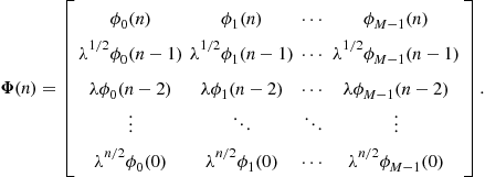 (12.149)
Note that the weighted least-squares cost function can be rewritten in terms of the vector ![]() , i.e.,
, i.e.,
![]() (12.150)
(12.150)
Now, we have to find the weight vector ![]() that minimizes (12.150). The gradient of
that minimizes (12.150). The gradient of ![]() with relation to
with relation to ![]() is given by
is given by
![]() (12.151)
(12.151)
where as usual, ![]() (resp.,
(resp., ![]() ) for complex (resp., real) data. Defining
) for complex (resp., real) data. Defining
![]() (12.152)
(12.152)
![]() (12.153)
(12.153)
in which ![]() is defined as before, (12.151) can be rewritten as
is defined as before, (12.151) can be rewritten as
![]() (12.154)
(12.154)
Equating ![]() to the null vector, we get the normal equations
to the null vector, we get the normal equations
![]() (12.155)
(12.155)
Note that these are a deterministic version of the normal equations we saw in Section 1.12.2.1. Therefore, to minimize ![]() , the weight vector
, the weight vector ![]() must satisfy
must satisfy
![]() (12.156)
(12.156)
which requires the computation of the inverse correlation matrix ![]() at each time instant. Note that this is only valid if
at each time instant. Note that this is only valid if ![]() is nonsingular. In particular, the inverse does not exist if
is nonsingular. In particular, the inverse does not exist if ![]() (Box 3). Assuming
(Box 3). Assuming ![]() and that the signals
and that the signals ![]() and
and ![]() are jointly stationary and ergodic, we obtain the following steady-state relations
are jointly stationary and ergodic, we obtain the following steady-state relations
![]()
Therefore, the deterministic normal equations converge to the stochastic normal equations when ![]() , and the weight vector obtained from (12.156) converges to the Wiener solution, i.e.,
, and the weight vector obtained from (12.156) converges to the Wiener solution, i.e.,
![]() (12.157)
(12.157)
We should mention that with ![]() the convergence rate of RLS goes to zero, i.e., it loses the ability to follow the statistical variations of the observed data. An equivalent result is obtained for LMS or NLMS when the fixed step-size
the convergence rate of RLS goes to zero, i.e., it loses the ability to follow the statistical variations of the observed data. An equivalent result is obtained for LMS or NLMS when the fixed step-size ![]() or
or ![]() is replaced by
is replaced by ![]() [39].
[39].
The computational cost of (12.156) is high due to the computation of the inverse matrix. In order to solve the normal equations in real-time and with less cost, we should rewrite (12.152) and (12.153) as recursions, i.e.,
![]() (12.158)
(12.158)
and
![]() (12.159)
(12.159)
with initializations ![]() and
and ![]() , where
, where ![]() is a small positive constant. Note that (12.159) is identical to (12.153), but (12.158) leads to the estimate
is a small positive constant. Note that (12.159) is identical to (12.153), but (12.158) leads to the estimate
![]() (12.160)
(12.160)
and therefore the initialization guarantees the existence of the inverse at all instants. For ![]() , the initialization
, the initialization ![]() is forgotten and (12.158) becomes close to (12.152) as
is forgotten and (12.158) becomes close to (12.152) as ![]() increases. Furthermore, if you want the algorithm to forget quickly the initialization, besides using
increases. Furthermore, if you want the algorithm to forget quickly the initialization, besides using ![]() , you should choose
, you should choose ![]() small (
small (![]() large). Note however that a certain amount of regularization may be useful in practice, to avoid problems when the input signal has long stretches with low power.
large). Note however that a certain amount of regularization may be useful in practice, to avoid problems when the input signal has long stretches with low power.
In order to obtain a recursion for the inverse matrix ![]() , we can use the matrix inversion lemma (Box 3) by comparing (12.138) with (12.158) and identifying
, we can use the matrix inversion lemma (Box 3) by comparing (12.138) with (12.158) and identifying
![]()
Thus, using (12.139), we obtain
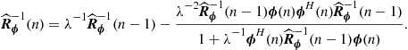 (12.161)
Defining ![]() , with some algebraic manipulations in (12.161), we arrive at
, with some algebraic manipulations in (12.161), we arrive at
 (12.162)
with initialization ![]() . This equation allow us to compute the inverse correlation matrix in a recurrent form, avoiding the explicit computation of a matrix inverse. However, the implementation of (12.162) in finite precision arithmetic requires some care to avoid numerical problems, as explained in Section 1.12.3.3.1.
. This equation allow us to compute the inverse correlation matrix in a recurrent form, avoiding the explicit computation of a matrix inverse. However, the implementation of (12.162) in finite precision arithmetic requires some care to avoid numerical problems, as explained in Section 1.12.3.3.1.
To simplify the following equations, it is convenient to define the column vector
![]() (12.163)
(12.163)
which is the so-called Kalman gain. Thus, (12.162) can be rewritten as
![]() (12.164)
(12.164)
Using (12.164) and some algebraic manipulations in (12.163), we arrive at
 (12.165)
Thus, using (12.159) and (12.165) in (12.156), the weight vector ![]() can also be computed recursively, i.e.,
can also be computed recursively, i.e.,
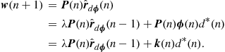 (12.166)
Replacing (12.164) in (12.166), we arrive at
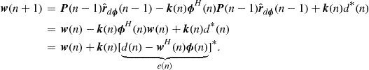 (12.167)
The RLS algorithm was derived here as an exact solution for the least-squares problem. However, it also can be interpreted as a quasi-Newton algorithm assuming the instantaneous approximation for the gradient vector as in (12.135) and considering ![]() as an approximation for the inverse Hessian matrix. Replacing these approximations in (12.134), we arrive at the same stochastic recursion (12.167).
as an approximation for the inverse Hessian matrix. Replacing these approximations in (12.134), we arrive at the same stochastic recursion (12.167).
The RLS algorithm is summarized in Table 12.5. Its computational cost increases with ![]() , much faster than those of LMS and NLMS. Different ways of carrying out the calculations may result in a slightly different computational cost, but all with the same order of magnitude, i.e.,
, much faster than those of LMS and NLMS. Different ways of carrying out the calculations may result in a slightly different computational cost, but all with the same order of magnitude, i.e., ![]() . Performing the calculations in the following order [3]:
. Performing the calculations in the following order [3]:

the conventional RLS requires ![]() real multiplications,
real multiplications, ![]() real additions, and one real division per iteration for complex-valued signals. For real-valued data, it requires
real additions, and one real division per iteration for complex-valued signals. For real-valued data, it requires ![]() real multiplications,
real multiplications, ![]() real additions, and one real division per iteration. Note that the quantities inside brackets were computed in previous steps.
real additions, and one real division per iteration. Note that the quantities inside brackets were computed in previous steps.

1.12.3.3.1 Practical implementation of RLS
The RLS algorithm must be implemented carefully, because it is sensitive to numerical errors, which may accumulate and make the algorithm unstable. The problem can be understood intuitively as follows. In the conventional RLS algorithm, the inverse of the autocorrelation matrix is computed recursively by (expanding (12.161))
![]()
i.e., as the difference between two positive (semi-) definite matrices. Note that, since ![]() , the factor multiplying the current
, the factor multiplying the current ![]() is
is ![]() . In infinite precision arithmetic, any growth due to this factor will be compensated by the second term. However, in finite precision arithmetic this compensation may not take place, and the factor
. In infinite precision arithmetic, any growth due to this factor will be compensated by the second term. However, in finite precision arithmetic this compensation may not take place, and the factor ![]() may make the recursion numerically unstable—usually, what happens is that
may make the recursion numerically unstable—usually, what happens is that ![]() looses its positive character, so the matrix will have a negative eigenvalue, which in its turn leads to the divergence of the coefficients. Thus, to avoid problems one would need to guarantee that
looses its positive character, so the matrix will have a negative eigenvalue, which in its turn leads to the divergence of the coefficients. Thus, to avoid problems one would need to guarantee that ![]() stays symmetric and positive-definite for all time instants
stays symmetric and positive-definite for all time instants ![]() (these properties are known as backward consistency of RLS [40,41]). Symmetry can be guaranteed by computing only the upper or lower triangular part of
(these properties are known as backward consistency of RLS [40,41]). Symmetry can be guaranteed by computing only the upper or lower triangular part of ![]() , and copying the result to obtain the rest of elements. However, it is also necessary to guarantee positive-definiteness. Reference [42] describes how this can be achieved.
, and copying the result to obtain the rest of elements. However, it is also necessary to guarantee positive-definiteness. Reference [42] describes how this can be achieved.
Due to the fast convergence rate of RLS, a large literature is devoted to finding numerically stable and low-cost (i.e., ![]() ) versions of RLS. This is not an easy problem, that required the work of numerous researchers to be solved. Nowadays the user has a very large number of different versions of RLS to choose from. There are versions with formal proofs of stability, versions that work well in practice, but without formal proofs, versions with
) versions of RLS. This is not an easy problem, that required the work of numerous researchers to be solved. Nowadays the user has a very large number of different versions of RLS to choose from. There are versions with formal proofs of stability, versions that work well in practice, but without formal proofs, versions with ![]() complexity, and versions with
complexity, and versions with ![]() complexity. The interested reader can find more references in Section 1.12.5.1.2.
complexity. The interested reader can find more references in Section 1.12.5.1.2.
One approach to ensure the consistency of ![]() uses a property of symmetric and positive-definite matrices (see Box 3): Cholesky factorizations. A symmetric and positive-definite matrix
uses a property of symmetric and positive-definite matrices (see Box 3): Cholesky factorizations. A symmetric and positive-definite matrix ![]() may always be factored as
may always be factored as
![]() (12.168)
(12.168)
where ![]() is a lower triangular
is a lower triangular ![]() matrix, called Cholesky factor of
matrix, called Cholesky factor of ![]() . Thus, an algorithm that computes
. Thus, an algorithm that computes ![]() instead of
instead of ![]() can avoid the numerical instability of the conventional RLS algorithm. There are many algorithms based on this main idea; for some of them a precise stability proof is available [40]. A recent and very complete survey of QR-RLS algorithms is available in [43].
can avoid the numerical instability of the conventional RLS algorithm. There are many algorithms based on this main idea; for some of them a precise stability proof is available [40]. A recent and very complete survey of QR-RLS algorithms is available in [43].
Another approach is available when the regressor sequence ![]() has shift structure. In this case, it is possible to derive lattice-based RLS filters that are in practice stable, although no formal proof is available at this time, as described, for example, in [5].
has shift structure. In this case, it is possible to derive lattice-based RLS filters that are in practice stable, although no formal proof is available at this time, as described, for example, in [5].
A more practical solution for the implementation of the RLS algorithm was proposed recently in [44]. This approach avoids propagation of the inverse covariance matrix, using an iterative method to solve (12.155) at each step. The computational complexity is kept low by using the previous solution as initialization, and by restricting the majority of the multiplications to multiplications by powers of two (which can be implemented as simple shifts). See Section 1.12.5.1.3.
1.12.3.4 Comparing convergence rates
To compare the convergence of LMS, NLMS, and RLS, we show next two examples. In Example 1, we consider a system identification application and in Example 2, we use these algorithms to update the weights of an equalizer.
As we will see in more detail in Section 1.12.4, adaptive filters are compared based on how well they handle different classes of signals. For example, we could be interested in seeing how two filters handle white noise, or how they handle a certain level of correlation at the input. Given the stochastic nature of the inputs, the performance measures are defined in terms of averaged cost functions, most commonly the mean-square error (MSE), that is, the average of ![]() over all possible inputs in a given class. These averages can be computed theoretically, as we show in Section 1.12.4, or via simulations.
over all possible inputs in a given class. These averages can be computed theoretically, as we show in Section 1.12.4, or via simulations.
For example, the MSE as a function of time, that is, the curve ![]() , is called a filter’s learning curve. A comparison of learning curves obtained theoretically and from simulations can be seen in Figure 12.30 further ahead. When simulations are used, one runs a filter
, is called a filter’s learning curve. A comparison of learning curves obtained theoretically and from simulations can be seen in Figure 12.30 further ahead. When simulations are used, one runs a filter ![]() times for an interval of
times for an interval of ![]() samples, starting always from the same conditions. For each run
samples, starting always from the same conditions. For each run ![]() , the error
, the error ![]() is computed for
is computed for ![]() , and one obtains the so-called ensemble-average learning curve
, and one obtains the so-called ensemble-average learning curve

Usually the ensemble-average learning curve will be a reasonable approximation of the true learning curve for a reasonably small value of ![]() (say, from
(say, from ![]() to
to ![]() ), but in some situations this may not be true—see [45,46] for examples and a detailed explanation.
), but in some situations this may not be true—see [45,46] for examples and a detailed explanation.
Example 1
The aim of this example is to identify the system ![]() , assuming that the regressor
, assuming that the regressor ![]() is obtained from a process
is obtained from a process ![]() generated with a first-order autoregressive model, whose transfer function is
generated with a first-order autoregressive model, whose transfer function is ![]() . This model is fed with an i.i.d. Gaussian random process with unitary variance. Moreover, additive i.i.d. noise
. This model is fed with an i.i.d. Gaussian random process with unitary variance. Moreover, additive i.i.d. noise ![]() with variance
with variance ![]() is added to form the desired signal.
is added to form the desired signal.
Considering an adaptive filter with ![]() coefficients, we can obtain a contour plot of the mean-square error cost as a function of
coefficients, we can obtain a contour plot of the mean-square error cost as a function of ![]() and
and ![]() as shown in Figure 12.25. The animations in Figure 12.25 illustrate the behavior of LMS
as shown in Figure 12.25. The animations in Figure 12.25 illustrate the behavior of LMS ![]() , NLMS
, NLMS ![]() , and RLS
, and RLS ![]() initialized at
initialized at ![]() . The correspondent curves of MSE along the iterations, estimated from the ensemble-average of 1000 independent runs, are shown in Figure 12.26. As expected for a colored input signal, RLS converges much faster than NLMS and LMS. NLMS converges faster than LMS and achieves the solution through a different path. To obtain a good behavior of NLMS in this example, we had to choose a relatively large regularization factor
. The correspondent curves of MSE along the iterations, estimated from the ensemble-average of 1000 independent runs, are shown in Figure 12.26. As expected for a colored input signal, RLS converges much faster than NLMS and LMS. NLMS converges faster than LMS and achieves the solution through a different path. To obtain a good behavior of NLMS in this example, we had to choose a relatively large regularization factor ![]() . This is always necessary when NLMS is used with few coefficients since in this case,
. This is always necessary when NLMS is used with few coefficients since in this case, ![]() has a high probability of becoming too close to zero and de-stabilizing the algorithm. This is shown in the analysis of Section 1.12.4.
has a high probability of becoming too close to zero and de-stabilizing the algorithm. This is shown in the analysis of Section 1.12.4.
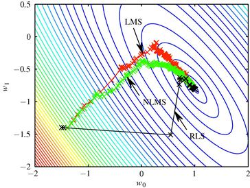
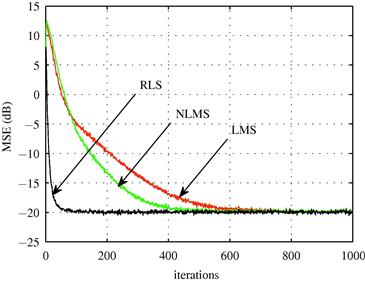
Example 2
Now, we assume the transmission of a QPSK (quadrature phase shift-keying) signal, whose symbols belong to the alphabet ![]() . This signal suffers the effect of the channel (taken from [47])
. This signal suffers the effect of the channel (taken from [47])
![]() (12.169)
(12.169)
and of additive white Gaussian noise (AWGN) under a signal-to-noise ratio (SNR) of ![]() . The equalizer is an adaptive filter with
. The equalizer is an adaptive filter with ![]() coefficients initialized with zero and the desired signal is the transmitted sequence delayed by
coefficients initialized with zero and the desired signal is the transmitted sequence delayed by ![]() samples (go back to Figure 12.16 to see the equalization scheme). The adaptation parameters
samples (go back to Figure 12.16 to see the equalization scheme). The adaptation parameters ![]() were chosen in order to obtain the same steady-state performance of LMS, NLMS, and RLS (note that with a longer filter, the regularization parameter
were chosen in order to obtain the same steady-state performance of LMS, NLMS, and RLS (note that with a longer filter, the regularization parameter ![]() can be much smaller than in the previous example). Figure 12.27 shows the MSE along the iterations, estimated from the ensemble-average of 1000 independent runs. Again, RLS presents the fastest convergence rate, followed by NLMS and LMS. These algorithms achieve the same steady-state MSE and therefore, present the same performance after convergence, which can be observed in Figure 12.28 where the equalizer output signal constellations are shown. The Matlab file used in this simulation is available at http://www.lps.usp.br.
can be much smaller than in the previous example). Figure 12.27 shows the MSE along the iterations, estimated from the ensemble-average of 1000 independent runs. Again, RLS presents the fastest convergence rate, followed by NLMS and LMS. These algorithms achieve the same steady-state MSE and therefore, present the same performance after convergence, which can be observed in Figure 12.28 where the equalizer output signal constellations are shown. The Matlab file used in this simulation is available at http://www.lps.usp.br.

Figure 12.27 MSE along the iterations for LMS ![]() , NLMS
, NLMS ![]() , and RLS
, and RLS ![]() ,
, ![]() initialized at
initialized at ![]() ; QPSK,
; QPSK, ![]() , and ensemble-average of 1000 independent runs; equalization of the channel (12.169).
, and ensemble-average of 1000 independent runs; equalization of the channel (12.169).
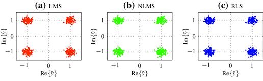
Figure 12.28 Equalizer output signal constellations after convergence for (a) LMS ![]() , (b) NLMS
, (b) NLMS ![]()
![]() , and (c) RLS
, and (c) RLS ![]() ; initialized at
; initialized at ![]() ; QPSK,
; QPSK, ![]() ; equalization of the channel (12.169).
; equalization of the channel (12.169).