
All-composite superstructures for accelerated bridge construction
H.S. Ji, Daewon University College, Republic of Korea
W. Song and Z.J. Ma, University of Tennessee at Knoxville, USA
Abstract:
This chapter presents the design, manufacture, installation, and in-service structural performance of an all-composite sandwich bridge superstructure for accelerated bridge construction (ABC). The superstructure is made of fiber-reinforced polymer (FRP). The discussions about the manufacture and installation include construction details when the FRP superstructure is implemented in practice. The assessment of the in-service structural performance may provide baseline data for the capacity rating and serve as part of the long-term performance monitoring of the FRP superstructure. Finally, this chapter explains why all-composite superstructures for ABC can be economically competitive in the future.
Key words
accelerated bridge construction; capacity rating; fiber-reinforced polymer (FRP) composites; long-term performance; sandwich bridge superstructure
6.1 Introduction
Recently, a main concern in bridge engineering had been the rehabilitation and reconstruction of deteriorated bridge members. Accelerated bridge construction (ABC) can overcome the shortcomings of traditional construction methods, which are typically labor-intensive and time-consuming. ABC can minimize disruption to public communities and save indirect costs associated with detouring traffic. Concrete members prefabricated in factory are often utilized in ABC, where the connections of prefabricated concrete members have been extensively studied in recent years (Li et al. 2010a, 2010b; Ma et al. 2012a, 2012b; Zhu et al. 2012a, 2012b). As alternatives to prefabricated concrete members, bridge superstructures entirely made of advanced composites or fiber-reinforced polymer (FRP) are also potential solutions to ABC, due to the following advantages of the materials:
• Light weight – FRP superstructures weigh about 25% or less of a conventional reinforced concrete superstructure. Therefore, FRP composites reduce the dead load of a superstructure significantly. Reduction of dead load can increase the rating factor when capacity rating of a bridge is performed. Since capacity rating of a bridge is proportional to the rating factor, the load carrying capacity of a superstructure reconstructed or rehabilitated with FRP composites may be re-rated to its original design load.
• Durability – Corrosion of steel reinforcement in concrete is the leading cause of deterioration of conventional concrete superstructures. Steel reinforcement is susceptible to oxidation when exposed to deicing salt and other chlorides. Compared to conventional materials, FRP composites provide high resistance to corrosion. Therefore, less maintenance may be required for FRP superstructures.
• Rapid Installation – Factory fabrication and modular construction of FRP superstructures allows rapid installation on construction sites. Installation of FRP superstructures in bridges with high traffic volume can substantially reduce the construction time of superstructures to half when compared to the labor-intensive and time-consuming construction process of a conventional cast-in-place concrete superstructure. As a result, disruption to communities, and indirect costs associated with detouring traffic, can be minimized by FRP superstructures.
• High Specific Stiffness/Strength – Advanced composites offer the advantages of high stiffness-to-weight ratios (specific stiffness) and strength-to-weight ratios (specific strength) when compared to conventional construction materials. Therefore, they can provide good combinations of strength/stiffness and weight for bridge superstructures.
• Lower Life-cycle Cost – A life-cycle cost usually consists of an initial construction cost and maintenance cost. Since FRP superstructures are expected to have good long-term durability and require little maintenance, they can be more cost-effective in service life than bridge superstructures with reinforced concrete.
In the United States, there are more than 40 bridge superstructures with FRP composites (Triandafilou and O’Connor,2009). No-Name Creek Bridge built in Russell, Kansas, was the first all-FRP bridge superstructure in the US (Plunkett, 1997). The FRP superstructure had a sandwich construction with honeycomb cores. Tech 21, the Smith Road Bridge built in Butler County, Ohio, was the third all-FRP superstructure in the US (Farhey, 2005). New York State Department of Transportation built an FRP superstructure in a demonstration project that had a cell core system providing stiffness in two directions (Alampalli, 2006). In other countries, all-composite superstructures have also been utilized in bridge construction. An FRP superstructure was installed and opened to the public in Yeongwol, Gangwon-Do, Korea in 2002 (Ji et al., 2007). The bridge superstructure was a sandwich structure with corrugated cores that could contribute significantly to the stiffness in the selected direction compared with other cores.
The projects above demonstrate how advanced composites or FRP materials were implemented in new bridge construction, or accelerated the rehabilitation of deteriorated bridges. Research on FRP superstructures indicates that their design should be controlled by stiffness rather than strength (Triandafilou and O’Connor, 2009). Although the advantages of FRP composites are recognized, their application in bridges needs further investigation. In fact, a number of technical challenges concerning design methods, connection details, dynamic effects, and long-term performance still remain unsolved. This chapter demonstrates structural analysis and design, manufacture and installation, and in-service structural evaluation of an FRP superstructure to consider these challenges. Finally, costs of the FRP superstructure are compared to those of reinforced concrete bridge superstructures.
6.2 Structural analysis and design
When designing all-composite bridge superstructures, designers can tailor FRP materials and structural configurations of superstructures to meet design requirements. As an example, the design of a two-lane FRP superstructure is discussed in this section. The FRP superstructure is now in service in South Korea, and has a sandwich construction (Ji et al., 2010). Corrugated cores are sandwiched between top facing and bottom facing. The sandwich construction in this study can reduce weight and provide significant stiffness in the selected direction. The discussion in this section includes design requirements, material selection, preliminary design based on design requirements, and detailed design of the cross-section.
6.2.1 Design requirements
The design of FRP superstructures is stiffness-oriented (Federal Highway Administration, 2011). Although no official specifications are available for the deflection limit of FRP superstructures, general design guidelines for conventional bridge superstructures are provided by the AASHTO LRFD Bridge Design Specifications (AASHTO, 2010). The AASHTO’s requirement for the stiffness of bridge superstructures with conventional materials is that the maximum deflection due to vehicular live loads should not exceed 1/800 of the bridge span length.
The criterion above was used to design the FRP superstructure in this chapter. The FRP superstructure in this chapter was expected to be in service in South Korea. As a result, the design vehicular live load in this study was consistent with Ministry of Construction and Transportation (MOCT) (2000a). As for the strength requirements, the maximum strain under service load should be limited to 20% of the ultimate strain. Laminate failure prediction was based on the first-ply failure criterion.
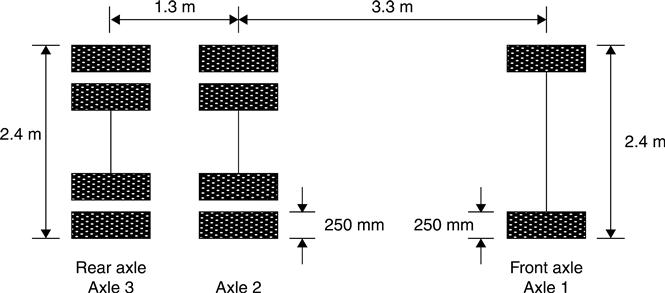
For a simply-supported bridge with span less than 44 m, the standard design truck load DB-24 produces higher moment and deflection than the design lane load (MOCT, 2000a). A DB-24 truck load is approximately 1.3 times heavier than the HS-20 truck load specified in AASHTO LRFD Bridge Design Specifications (2010). One standard design truck load DB-24 with tire contact areas, as shown in Fig. 6.1 (MOCT, 2000b), was assumed to be the design live load. The weight of a DB-24 truck is 423 kN.
6.2.2 Materials and lamina design
Superstructures with FRP composites including the one in this study can be characterized at three levels: the lamina level (a single ply), the laminate level (multiple plies), and the structural level (Altenbach et al., 2004). This section focuses on the materials and lamina design. The design at the latter two levels will be addressed in the following sections.
The primary constituents of FRP composites are fibers and resin matrices. In FRP bridge superstructures, glass fibers are mainly used as fiber reinforcement, and polyester or vinyl ester is the most widely used resin matrix. Their combinations can be the most cost-effective in current practice. In this study, E-glass fibers and vinyl ester resin were chosen as the main constituents for the all-FRP superstructure for ABC. Their material properties are given in Table 6.1 (Ji et al., 2010).
Table 6.1
Properties of constituent materials
| Material | E (GPa) | G (GPa) | υ | ρ (kN/m3) |
| E-glass fiber | 72.4 | 27.6 | 0.22 | 25.4 |
| Vinyl ester resin | 3.91 | 1.38 | 0.37 | 12.4 |

E is the Young’s modulus; G is the shear modulus; υ is the Poisson’s ratios; ρ is the density.
To design a superstructure with FRP composites, it is necessary to know the mechanical properties of a single ply or a lamina made of fiber reinforcement and resin matrix. The properties of a lamina with unidirectional fibers can be predicted from properties of fibers and resin matrix according to micro-mechanics models based on several simple rules of mixtures. Most calculations about the properties of a unidirectional lamina depend on the volume fraction of fibers and resin matrix. The fiber and matrix volume fractions, Vf and Vm, respectively, for a unidirectional lamina based on their weight fractions and densities are calculated in Equation [6.1].
[6.1]
where wf and wm are the weight fractions of fibers and resin matrix, ρf and ρm are the densities of fibers and resin matrix.
The mechanical properties of a unidirectional lamina with known fiber and matrix properties and their volume fractions can be calculated by simple rules of mixtures as shown in Equations [6.2]–[6.5].
[6.2]
[6.3]
[6.4]
[6.5]
where η0 is the efficiency factor of fibers – for unidirectional fibers, η0 is equal to 1.0; Ef and Em are the Young’s moduli of fibers and resin matrix, respectively; Gf and Gm are the shear moduli of fibers and resin matrix, respectively, and; υf and υm are the Poisson’s ratios of fibers and resin matrix, respectively.
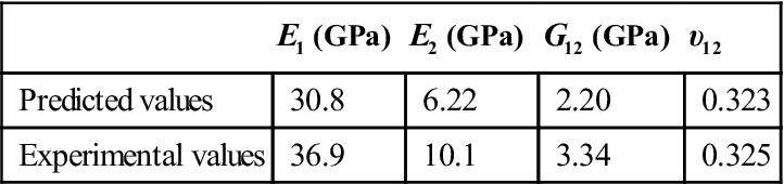
For the FRP sandwich superstructure in this study, the unidirectional laminae in it have wf equal to 57% and wm equal to 43%. Assuming that there are no voids in the FRP laminae, their mechanical properties predicted using Equations [6.1]–[6.5] are shown in Table 6.2 (Ji et al., 2010).
Table 6.2
Mechanical properties of a unidirectional FRP lamina
| E1 (GPa) | E2 (GPa) | G12 (GPa) | υ12 | |
| Predicted values | 30.8 | 6.22 | 2.20 | 0.323 |
| Experimental values | 36.9 | 10.1 | 3.34 | 0.325 |
The FRP laminae discussed here, with various orientations, were used to construct the laminates for the facings and core walls of the FRP superstructure. The details about the lay-ups of the laminates were determined based on the preliminary and detailed design, and will be discussed in the following sections. In design, it is often necessary to have a preliminary estimation of the thickness of a laminate. The thickness that can be achieved is related to the mass of the materials used in the laminate. The thickness of a laminate can be predicted using a thickness constant in Equation [6.6]:
[6.6]
The thickness constant can be calculated from a given density in Equation [6.7]:
[6.7]
6.2.3 Preliminary design
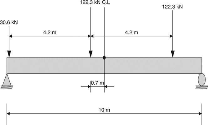
At the preliminary design stage, the required material and section properties for the FRP sandwich superstructure were determined based on the design load mentioned in Section 6.2.1. They should be obtained to guarantee that the midspan deflection Δ under the maximum live-load effect would not exceed 1/800 of the bridge span length. The FRP superstructure discussed here was a simply-supported bridge with a single span and two traffic lanes. It was 10 m long by 8 m wide. The placement of three wheel loads from the DB-24 truck is shown in Fig. 6.2. It was determined by the influence line to maximize the moment effect at midspan (Ji et al., 2010). The loads in Fig. 6.2 are the wheel loads multiplied by the impact factor of 1.3.
At the preliminary design stage, it is desirable to perform the design without invoking finite element analysis (FEA) (Triandafilou and O’Connor, 2009). The properties of the top and bottom facings and the depth of the FRP superstructure could be designed by the following two simplified structural analysis methods without using FEA. In this study, the subscripts x and y denote the transverse direction and span direction, respectively.
Principle of virtual work
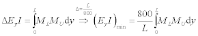
According to the principle of virtual work, the required stiffness of the cross-section EyI times the midspan deflection Δ for the loading case shown in Fig. 6.2 could be calculated in Equation [6.8] (Ji et al., 2010). It should be noted that EyI is constant along the span length.
[6.8]
 [6.8]
[6.8]
where MU is the moment caused by the unit load acting at the midspan, ML is the moment caused by the actual loads, Ey is the Young’s modulus of the cross-section in the longitudinal direction, L is the bridge span length, and I is the moment of inertia of the superstructure’s cross-section.
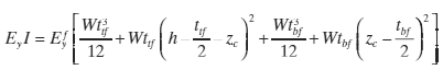
The FRP superstructure in this study has a sandwich construction. If the contribution of core walls to the moment of inertia I is neglected and the Young’s moduli of top and bottom facings in the longitudinal direction are assumed to be the same, the expression for EyI is given in Equation [6.9].
[6.9]
 [6.9]
[6.9]
where h is the depth of the superstructure, W is the width of the superstructure’s cross-section, ttf and tbf are the thickness of the top and bottom facing respectively, zc is the distance between the centroid of the superstructure’s cross-section and the extreme bottom fiber of bottom facing, and Efy is the Young’s modulus of the top and bottom facing in the longitudinal direction.
In order to satisfy the deflection limit for the FRP superstructure, the actual EyI should be larger than the required one (EyI)min. This relationship is indicated by Equation [6.10]. In practice, the material properties and thickness of the laminated facings and the depth of the FRP superstructure can be varied to satisfy Equation [6.10].
[6.10]
 [6.10]
Equivalent strip width
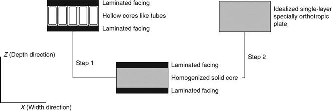
The preliminary design could be further refined by using the equivalent strip width for FRP superstructures (Song, 2012). The FRP superstructure in this study was directly treated as a 1-D beam on the principle of virtual work, so that its actual width was utilized in the previous calculation. This assumption should be modified because the FRP superstructure might behave like a 2-D plate instead of a 1-D beam. Further, Equations [6.8] and [6.9] neglected the deflection of the FRP superstructure due to out-of-plane shear deformation. Considering these problems, the design at the preliminary design stage could be improved by using the equivalent strip width to design the superstructure as a 1-D Timoshenko beam.
Typical FRP superstructures can be idealized as single-layer specially orthotropic plates (Davalos et al., 1996, 2001; Zhou, 2002). An example of the idealization from previous research is given in Fig. 6.3 (Zhou, 2002). At the preliminary design stage, the equivalent material properties of idealized orthotropic plates, including the one in this study, are not known. As is evidenced in Fig. 6.3, the equivalent material properties are influenced by the properties of FRP laminae and laminates, and structural configuration and geometry of FRP superstructures. Few of these factors are available at the preliminary design stage. However, reasonable assumptions can be made about the equivalent material properties of idealized orthotropic plates.
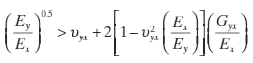
FRP superstructures in practice are typically less than 18.3 m and their width-to-span ratios are less than 1.5. Most of them have one lane or two lanes and equivalent material properties described below. The ratio of the two equivalent Young’s moduli Ex/Ey varies between 0.1 and 0.9. The equivalent major Poisson’s ratio υyx changes from 0.1 to 0.4. The ratio of the equivalent in-plane shear modulus Gyx to the equivalent Young’s modulus Ex is between 0.1 and 0.4. The ratio of the equivalent out-of-plane shear modulus Gxz to the equivalent Young’s modulus Ex, and the ratio of the equivalent out-of-plane shear modulus Gyz to the equivalent Young’s modulus Ey, are at least 0.025. The combination of Ex, Ey, Gyx, and υyx for an FRP superstructure usually satisfies the relationship in Equation [6.11].
[6.11]
 [6.11]
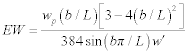
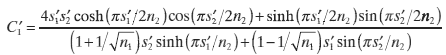
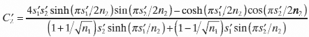
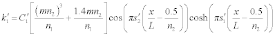
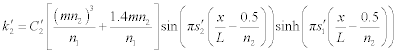
Considering the discussions above about practical FRP superstructures, the equivalent strip width for the preliminary design of FRP superstructures is given in Equations [6.12]–[6.19] (Song, 2012). It should be mentioned that in essence Equations [6.12]–[6.19] are simplifications of 2-D plate analysis. Therefore, each load on an FRP superstructure may correspond to an equivalent strip width. The equivalent strip width here is used to facilitate the midspan deflection calculation by Timoshenko beam theory, in which only loading conditions in the longitudinal or span direction are required. In the transverse direction, it is assumed that design live loads have symmetric distribution with respect to the centerlines of FRP superstructures. The symmetry can be utilized to reduce the number of equivalent strip width calculations at the preliminary design stage.
[6.12]
 [6.12]
[6.13]
[6.14]
 [6.14]
[6.15]
 [6.15]
[6.16]
 [6.16]
[6.17]
 [6.17]
[6.18]
 [6.18]
[6.19]
where EW is the equivalent strip width corresponding to a specific load, wp is the width of a pressure in the transverse direction, b is the distance from the center of a pressure to the closest support in the span direction, and a is the position of a pressure’s center in the transverse direction. L is the span length and W is the width of the superstructure. x is the coordinate of a point in the transverse direction at midspan. For one-lane FRP superstructures, x is suggested to be either W/2 or a. For multi-lane FRP superstructures, x is suggested to be either a or the coordinate of the center of each lane in the transverse direction.
Equations [6.12]–[6.19] only include three key parameters n1, n2, and υyx, which have significant influences on the equivalent strip width (Song, 2012). The actual values about Ex, Ey, Gyx, Gxz, and Gyz, which are not known and difficult to assume at the preliminary design stage, are not required for the calculation of the equivalent strip width. Consequently, these equations can avoid inconvenient 2-D plate design based on first-order shear deformation theory (FSDT) when the equivalent strip width from them is directly used with Timoshenko beam theory. It should be emphasized that Ex, Ey, Gyx, Gxz, and Gyz are the equivalent material properties of an idealized single-layer specially orthotropic plate. They are generally not equal to the material properties of a lamina or a laminate in an FRP superstructure, as is implied in Fig. 6.3. Their calculation may be referred to several research studies conducted previously (Davalos et al., 1996, 2001).
The equivalent strip width discussed here could be used to perform the preliminary design of the FRP sandwich superstructure in this study. Considering the properties of the FRP laminae in Table 6.2, n1 should be 6 or less if the contribution of core walls were neglected. At the beginning of the preliminary design, Ey was arbitrarily assumed as 6.0 GPa. υyx might be assumed as 0.3. The span-to-depth ratio was considered as 12 (Federal Highway Administration, 2011). To use Timoshenko beam theory in design, another assumption about the out-of-plane shear modulus Gyz should also be made, although this assumption had no impact on the equivalent strip width calculation. In this study, Gyz was Ey/40.
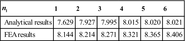
The midspan deflections at (W/4, L/2) predicted by Timoshenko beam theory with the equivalent strip width at several n1 are shown as the analytical results in Fig. 6.4 and Table 6.3. Correspondingly, the midspan deflections at (W/4, L/2) from FEA using the commercial package ABAQUS are also shown in Fig. 6.4. The maximum deflections from tire contact areas are shown in Table 6.3 to investigate the local deformation within these regions.
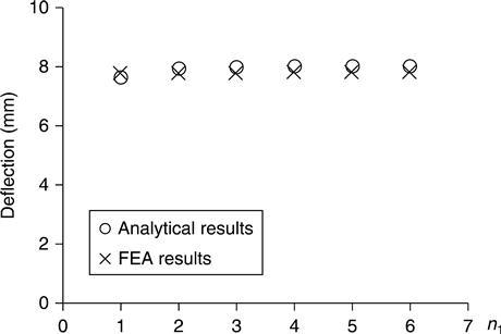
Table 6.3
Deflections at (W/4, L/2) and tire contact area (unit: mm)
| n1 | 1 | 2 | 3 | 4 | 5 | 6 |
| Analytical results | 7.629 | 7.927 | 7.995 | 8.015 | 8.020 | 8.021 |
| FEA results | 8.144 | 8.214 | 8.271 | 8.321 | 8.365 | 8.406 |
When the results in Fig. 6.4 and Table 6.3 were predicted, the placement of DB-24 truck loads in the span direction was the same as that in Fig. 6.2. In the transverse direction, two DB-24 trucks were considered, and each truck was symmetric with respect to the centerline of each lane. The modeling in FEA was consistent with FSDT. In FEA, Gyx/Ex was equal to 0.25 and Gxz/Ex was equal to 0.025. These two ratios did not affect the equivalent strip width and Timoshenko beam theory but did affect FSDT (Song, 2012).
Figure 6.4 shows that the equivalent strip width together with Timoshenko beam theory can be used to predict midspan deflections and perform the preliminary design of the FRP sandwich structure in this study. Table 6.3 indicates that the local deformation at tire contact areas is not significant enough to invalidate the 1-D Timoshenko beam design with the equivalent strip width discussed here. The maximum analytical deflection from Table 6.3 is about 1/1250 of the span length of the FRP sandwich superstructure. As a result, a cross-section whose Young’s modulus in the span direction Ey and depth h satisfy the relationship in Equation [6.20] is necessary to the FRP superstructure in this study. According to Fig. 6.3, Ey is a function of laminated facings and core walls. It also depends on the depth of the cross-section. For the FRP superstructure in this study, the material properties and thickness of the laminates in facings and cores and the depth can be varied to satisfy Equation [6.20].
[6.20]
It should be mentioned that the equivalent strip width from Equations [6.12]–[6.19] is also suitable to perform parametric study and design optimization. The procedure is explained as follows. The first two steps in the procedure are utilized in the example above. The remaining steps should be followed if parametric study and design optimization at the preliminary design stage are conducted without using FEA. Although Equations [6.12]–[6.19] appear to be complex, they can be conveniently utilized in a spreadsheet. Once a spreadsheet is set up, minor modifications are required to cover different cases in the parametric study.
1. Calculate the aspect ratio n2 from the geometry of an FRP superstructure and make an assumption about the depth. The span-to-depth ratio is suggested to be equal to 12.
2. Make an initial assumption about n1 and υyx. A reasonable assumption about n1 is 10, and υyx may be taken as 0.3. Then calculate the equivalent strip width for each load.
3. Assume that Gyz/Ey is 1/40, and then calculate the required Ey by Timoshenko beam theory based on the argument that the total midspan deflection under design live loads is equal to its limit.
4. Based on the calculated Ey, tailor FRP materials and design cross-sections.
5. Idealize the FRP superstructure as a single-layer specially orthotropic plate and update the equivalent properties Ey, Ex, υyx, Gyx, Gyz, and Gxz.
6. Based on the actual equivalent properties of the cross-section, update the equivalent strip width.
7. Modify laminates in components of the FRP superstructure and/or reduce the depth if predicted midspan deflections with the updated equivalent strip width are not close to the limit.
8. Repeat the process from Steps 5 to 7 until satisfactory results are achieved.
6.2.4 Detailed design
The FRP superstructure in this study has a sandwich structure with corrugated core walls. Besides the parameters influencing the relationship in Equation [6.10] or [6.20], several geometric factors of corrugated cores also affect the behavior of the superstructure. These geometric factors are the corrugation angle, the ratio of the core depth to core wall’s thickness, and the ratio of the pitch to core depth as shown in Fig. 6.5 (Libove and Hubka, 1951). All the parameters were determined based on a detailed design by FEA using the LUSAS software. In the detailed design, DB-24 trucks multiplied by the impact factor of 1.3 were considered as design live loads. The dead loads, including the self-weight of the superstructure and asphalt wearing surface with a thickness of 50 mm, were also considered in the design.
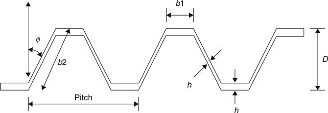
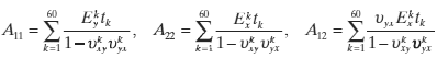
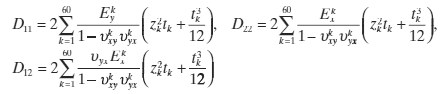
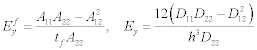
Based on the FEA, the final proposed section of the FRP sandwich superstructure with corrugated cores for manufacturing is shown in Fig. 6.6 (Ji et al., 2007, 2010). The FRP superstructure is 10 m in length, 8 m in width, and 0.94 m in depth. The superstructure’s cross-section is constant along the whole span. The lay-ups of the FRP laminae in Section 6.2.2 in the laminates for facings and core walls are shown in Table 6.4. The corrugation angle, the ratio of the core depth to core wall’s thickness, and the ratio of the pitch to core depth are selected to be 70°, 22, and 1.6, respectively. If the contribution of the core walls to flexural stiffness is neglected, it is straightforward to show that the geometry and construction in Table 6.4 can satisfy the relationship in Equations [6.10] and [6.20]. Considering the material properties in Table 6.2, the Efy and Ey in Equations [6.9] and [6.20] can be calculated according to Equations [6.21]–[6.23] (Bank, 2006; Barbero, 2010). The proposed section in Fig. 6.6 also satisfied the deflection limit in the FEA.
[6.21]
 [6.21]
[6.22]
 [6.22]
[6.23]
 [6.23]
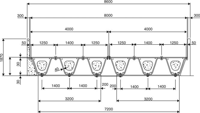
Table 6.4
Lay-up of the laminates for facings and core walls
| Components | Lamina lay-up | Ply thickness (mm) | No. of plies | Total thickness (mm) |
| Top facing | [0°/90°/90°/0°]15 | 0.5 | 60 | 30 |
| Core wall | [0°/45°/-45°/90°/mat]16 | 0.5 | 80 | 40 |
| Bottom facing | [0°/90°/90°/0°]15 | 0.5 | 60 | 30 |
where k denotes the kth lamina in the laminate for a facing, tk is the thickness of the kth lamina, zk is the distance between the centroid of the kth lamina and the centroid of the cross-section of the FRP superstructure, and Eky, Ekx, and υkyx are E1, E2, and υ12 for the kth lamina if its orientation is 0°, and are E2, E1, and υ21 for the kth lamina if its orientation is 90°.
The vehicle traffic barrier system should also be designed for the FRP superstructure at this stage. Many demonstration projects show that concrete barriers are mainly used to contain vehicles on FRP bridge decks. The embedded steel bars and grout are usually applied to construct and attach reinforced concrete barriers to FRP bridge decks. As a result, the components of the FRP decks, such as flanges and webs, are often partly damaged. In this study, an improved vehicle traffic barrier system separating barriers and the FRP superstructure, which is shown in Fig. 6.7 (Ji et al., 2010), was proposed for the FRP bridge construction. This barrier system was attached to the concrete abutment instead of attaching to the FRP superstructure. Consequently, it does not cause any damage to the FRP superstructure, such as local tearing of fibers and resin matrix. It will also make future barrier upgrading possible without damaging the FRP superstructure.

Currently, there is no design guidance for the barrier system used for this study. As a result, specifications from AASHTO LRFD (2010) were chosen to design it. The design force for the barrier system is related to the Test Levels 1–6 specified in AASHTO LRFD (2010). The choice of test level depends on several factors, such as bridge alignment, and traffic volume and speed. For the FRP superstructure in this study, Test Level 1 was chosen for the design of the barrier system. The load capacity for the barrier system in this study is 675 kN, which is larger than the 120 kN required by Test Level 1 (Ji et al., 2010). Consequently, this barrier system can be used for the FRP superstructure.
6.3 Manufacture and installation
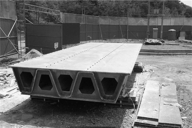
The FRP sandwich superstructure with corrugated cores was manufactured by commercial fabricators according to the detailed design drawing shown in Fig. 6.6. It consisted of two modular pieces, each 10 m long, 4 m wide, and 0.94 m deep. The modular pieces were the largest transportable units, due to shipping constraints. The FRP superstructure was completed by joining the two pieces on the field application site. Each modular piece consists of three components: top facing, corrugated cores, and bottom facing. All components were manufactured by a hand lay-up method. Facings were hand-laid and their thickness was approximately 30 mm according to Table 6.4. The corrugated core’s walls were hand-laid at room temperature on wood molds. Each wall contained 80 plies and the thickness was 40 mm. Then, internal transverse FRP frames were coated with adhesives and bonded to the inside surfaces of corrugated cores to provide stability and to maintain wall thickness. The transverse frames were also applied at the superstructure’s end supports to provide end rigidity for load transfer from the superstructure to the abutments. After their fabrication, the corrugated cores were hoisted onto bottom facings by a light duty crane. Then, M20 steel bolts with the spacing of 32 mm were used to fasten the facings to the corrugated cores. Figure 6.8 shows one finished modular piece of the FRP superstructure (Ji et al., 2010).
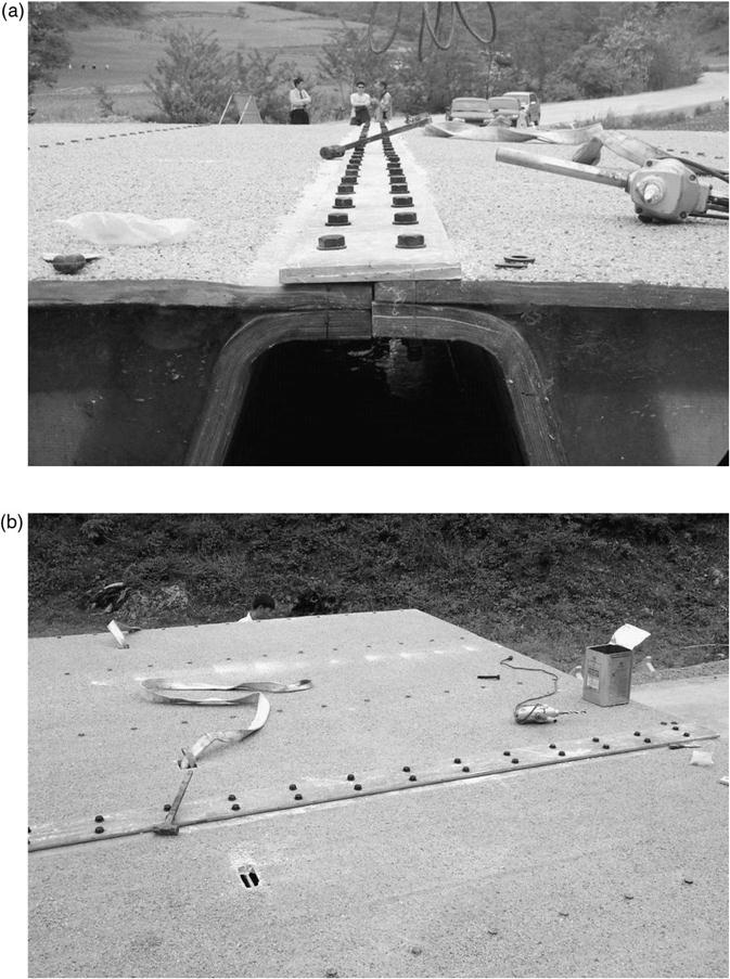
The two modular pieces were prefabricated in a factory and assembled on the construction site. Their top and bottom facings were bolted to FRP cover plates in the field. Figure 6.9 shows the connections of the modular pieces. Bolt diameter and bolt spacing were designed according to the EURO design code for bolting in FRP members (Eurocomp, 1996). Figure 6.10 shows the entire FRP bridge superstructure (Ji et al., 2010). In order to prevent the local deflection of the top facings between the corrugated cores, the hollow cells of the superstructure were later filled with expandable polyurethane foams.
In order to protect FRP superstructures from moisture and contamination, wearing surfaces such as polymer concrete and asphalt concrete could be utilized in practical construction. In the FRP superstructure of this study, asphalt concrete was used as the wearing surface. Epoxy-coated fine aggregate overlay was applied on the surface of the superstructure to avoid delamination between the asphalt wearing surface and the top facing. The epoxy-coated fine aggregate overlay was 0.88 mm thick. The asphalt concrete wearing surface was 50 mm thick. In terms of thermal behavior, the FRP materials could resist a temperature up to 175°C. There was no deformation over the superstructure’s surface due to the heat of the asphalt concrete.
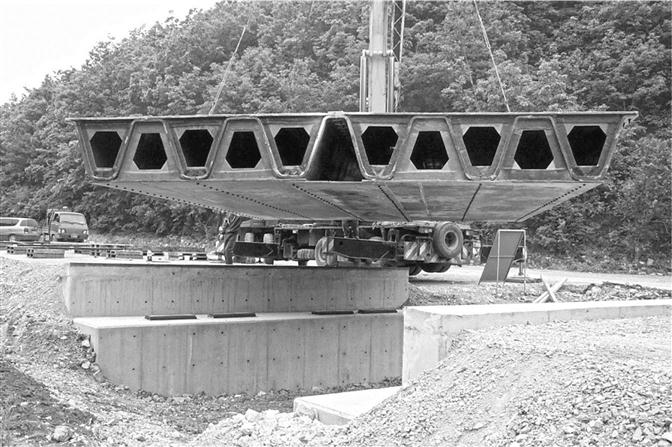
In this study, the FRP superstructure was easily placed on the concrete abutments using a light duty crane. The bridge seats were 50 mm thick neoprene pad shoes. In the actual construction, the neoprene shoes were adjusted to accommodate the unevenness of the superstructure’s bottom facing. Holes in the bottom facing of the superstructure were made to fit over two stainless steel threaded rods on each concrete abutment. The threaded rods acted as anchors to tie the superstructure to the concrete abutments and prevent uplift at the bridge supports. Expansion joints which were 10 mm wide were provided at the supports. Finally, the reinforced concrete barriers were built after the first field load testing of the FRP superstructure. The completed bridge is shown in Fig. 6.11 (Ji et al., 2010).

6.4 In-service structural performance evaluation
The primary goals of the in-service structural performance evaluation were to investigate if the FRP superstructure could satisfy the design requirements for stiffness and strength in Section 6.2.1. The results from the inservice structural performance evaluation could be utilized to investigate dynamic effects on the FRP superstructure and to perform capacity rating of the FRP superstructure as well.
6.4.1 Field testing
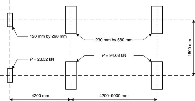
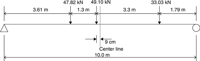
The field testing was conducted in 2002, 2004, and 2011. The bridge with the FRP superstructure was tested using one or two dump trucks, like the one shown in Fig. 6.12. The wheel weights of one dump truck used for the field testing in 2011 are shown in Fig. 6.13. The axle weights of the dump trucks for the field testing in 2002 and 2004 are given in previous research (Ji et al., 2007). Both static and dynamic tests were conducted in the field load testing. In static tests, the truck or trucks were placed at pre-marked positions shown in Fig. 6.13 to maximize the bending moment at midspan. The dynamic tests were conducted with the vehicle traveling over the bridge at speeds of 10–60 km/h. Static and dynamic tests consisted of four loading cases in which the truck or trucks are on the right lane (Load case 1 (LC1)), left lane (LC2), center lane (LC3), and two lanes (LC4) of the bridge.
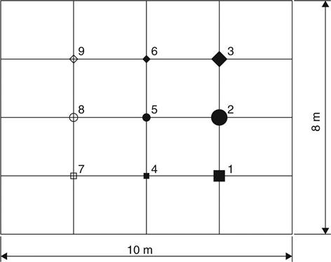
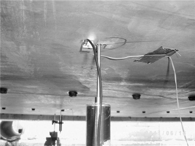
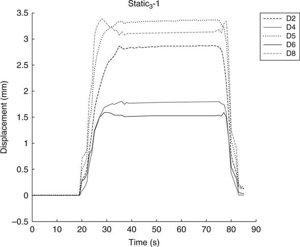
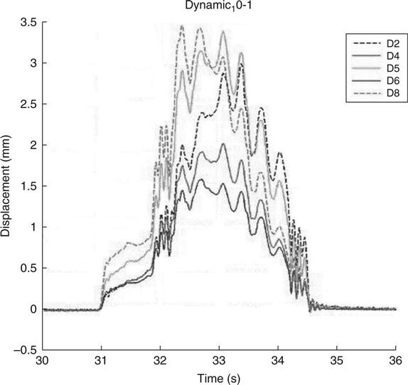
The FRP superstructure was instrumented with conventional strain gages and linear variable differential transformers (LVDTs) on its bottom surface. The numbering of the positions where strain gages and/or LVDTs might be applied is shown in Fig. 6.14. The positions were chosen to investigate responses at several points at midspan and quarterspan. Further, an accelerometer was instrumented at the Position 5 for the field load testing. Figure 6.15 illustrates the instrumentation of the accelerometer. Figures 6.16 and 6.17 show the results of static and dynamic displacements under the LC3 from the field load testing conducted in 2011. It is noteworthy that the letter ‘D’ before a number denotes the deflection at the point corresponding to the number.
6.4.2 Results and discussion
In order to investigate if the FRP superstructure satisfied the design requirements for stiffness and strength, the results from the field testing in 2002 should be invoked and compared with the deflection and strength limit. The field testing in 2002 was conducted before the FRP superstructure had the concrete barrier system and was opened to the public. The static responses measured in the LC3 by a loaded truck ‘crawling’ across the FRP bridge at about 5 km/h were used as a reference. The measured deflection at midspan was 4.72 mm, less than its design limit L/800, which was 12.5 mm in this study. The midspan bending strain in tension was 101.72 με at a truck load of 250.56 kN. It was less than the allowable strain, which was 20% of the failure strain 19 317 με obtained from the manufacturers’ data. The results above also verified that the FRP superstructure design should be controlled by stiffness rather than strength.
To study dynamic effects on the FRP superstructure, the data taken from the dynamic tests in 2002 under the LC3 at six speeds (10–60 km/h) were analyzed. The maximum dynamic deflection was measured to be 4.78 mm at the speed of 40 km/h. This value was just a little more than 4.72 mm, which was from the static test under the same loading case. The largest impact factor was 0.016, and it was relatively small compared to the value of 0.33 for the cases of conventional materials (AASHTO LRFD, 2010). The results above showed that the dynamic effects induced by the passage of the truck at various speeds were not of much significance. This conclusion was attributed to the difference between the natural frequency of the FRP superstructure and the forced frequency from the passing truck.
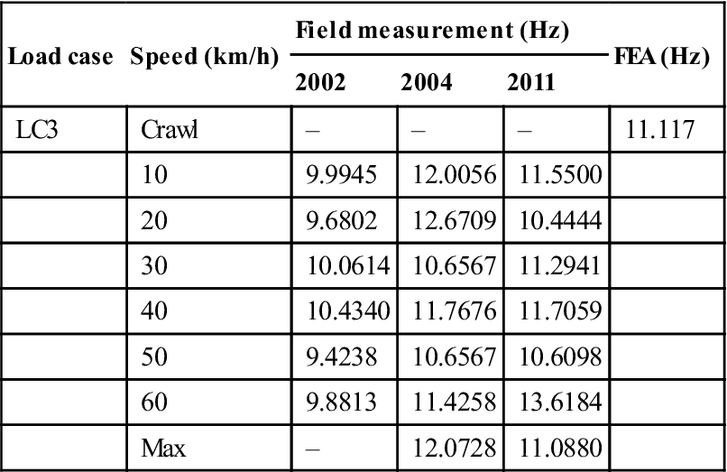
The damped natural frequencies from the test data obtained in 2002, 2004, and 2011 were calculated by using the fast Fourier transformation (FFT) analysis of the natural vibration part of acceleration components. An example of the FFT analysis using the data obtained in 2011 is shown in Fig. 6.18. Table 6.5 shows the comparison of the damped frequencies from the experimental results and FEA.
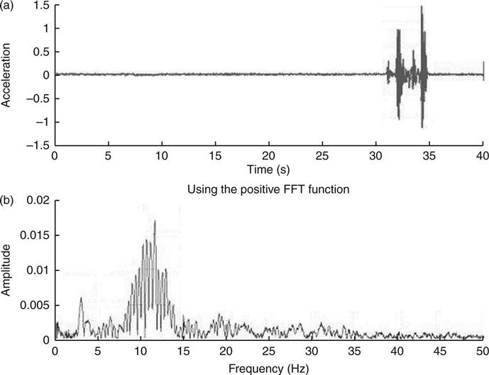
Table 6.5
| Load case | Speed (km/h) | Field measurement (Hz) | FEA (Hz) | ||
| 2002 | 2004 | 2011 | |||
| LC3 | Crawl | – | – | – | 11.117 |
| 10 | 9.9945 | 12.0056 | 11.5500 | ||
| 20 | 9.6802 | 12.6709 | 10.4444 | ||
| 30 | 10.0614 | 10.6567 | 11.2941 | ||
| 40 | 10.4340 | 11.7676 | 11.7059 | ||
| 50 | 9.4238 | 10.6567 | 10.6098 | ||
| 60 | 9.8813 | 11.4258 | 13.6184 | ||
| Max | – | 12.0728 | 11.0880 | ||
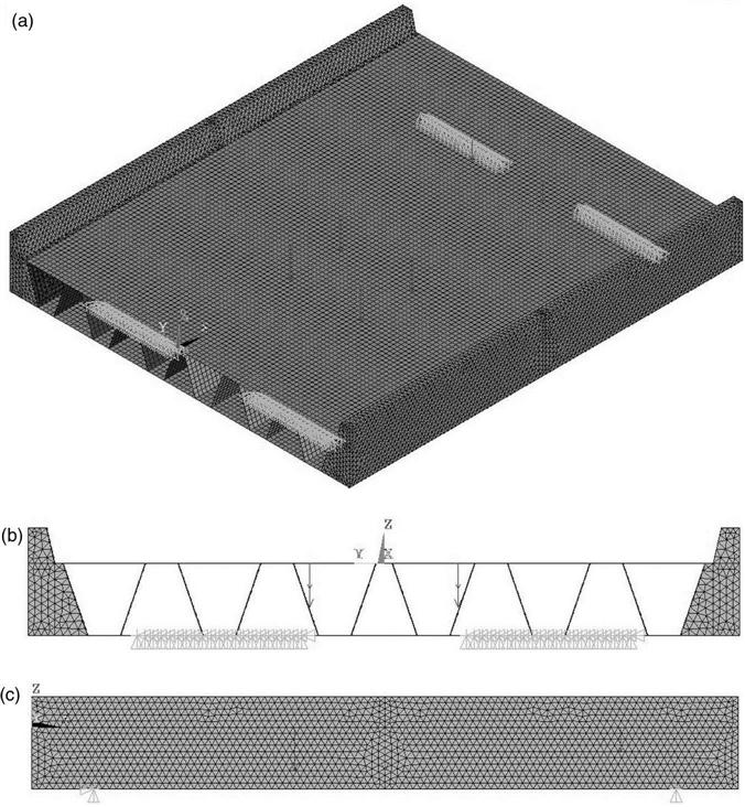
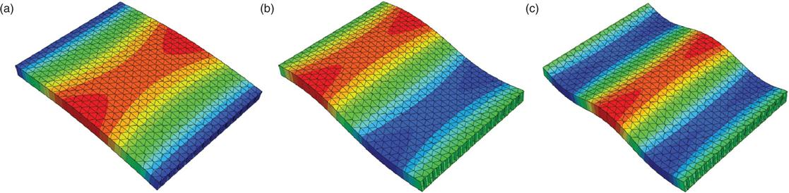
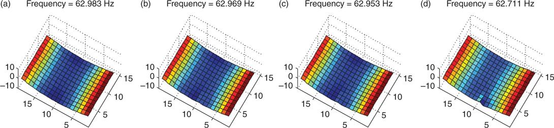
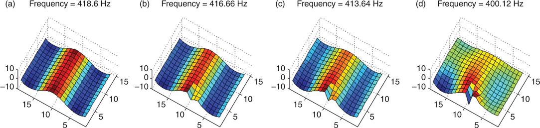
The recorded damped frequencies of the FRP superstructure are close to the predicted value of 10 Hz from f = 82L−0·9, where L is 10 m (Hayes et al., 2000). They are also close to the value calculated by the FEA shown in Fig. 6.19. The FEA in Fig. 6.19 was conducted by ANSYS software (ANSYS, 2005). Nine-node thick shell elements were used to model the FRP laminates in the FRP superstructure. In the finite element modeling, the material properties and fiber orientation of each lamina that constitutes a laminate were input for these shell elements. The boundary conditions were modeled as a pin and a roller at the end supports.
In 2002, the shear strength of the interfaces between the asphalt wearing surface and the surface of the superstructure was measured from shear tests. The shear strength values were within the range 0.35 to 0.61 MPa. They exceeded the required shear strength of 0.15 MPa for the interfaces between steel deck plates and asphalt wearing surfaces according to the specification for highway bridges in Korea (MOCT, 2000b). The measurement indicated that there was a good interface bond between the asphalt concrete wearing surface and the surface of the superstructure at that time. According to the field inspection in 2011, cracks between the asphalt concrete pavement and the FRP superstructure have been found. These cracks might be caused by decreased shear strength between the asphalt concrete pavement and the FRP superstructure.
6.4.3 Capacity rating
Recently, interest in field load testing of highway bridges has partly resulted from the large number of deteriorated bridges with posted load limits that are below standard truck weights. Field load testing is an attractive tool to perform capacity rating of a bridge (Stallings and Yoo, 1993). The results of the field testing in this study are used to refine bridge rating calculations.
The formula for capacity rating of an in-service bridge with conventional materials is given in Equation [6.24].
[6.24]
where RF, ks, and Pr denote the rating factor, stress modification coefficient, and test truck loading, respectively, and P is the capacity of the bridge.
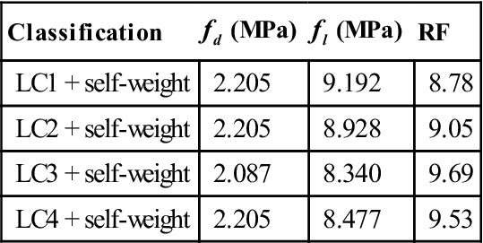
For the FRP superstructure in this study, the rating factor (RF) in Equation [6.24] could be determined based on the allowable stress method. Its calculation is given in Equation [6.25].
[6.25]
where fa is the allowable stress, fd is the stress due to dead loads, fl is the maximum live-load stress produced by the standard vehicle, and i is the impact factor that accounts for dynamic loading effects. The fa based on experimental data is 107.16 MPa in this study. The fd and fl could be determined from FEA. According to MOCT (2000a), the impact factor i could be calculated based on Equation [6.26]. L in Equation [6.26] is the span length in meters. A summary of the RF obtained based on Equation [6.25] and Fig. 6.13 is shown in Table 6.6.
[6.26]
Table 6.6
| Classification | fd (MPa) | fl (MPa) | RF |
| LC1 + self-weight | 2.205 | 9.192 | 8.78 |
| LC2 + self-weight | 2.205 | 8.928 | 9.05 |
| LC3 + self-weight | 2.087 | 8.340 | 9.69 |
| LC4 + self-weight | 2.205 | 8.477 | 9.53 |
The stress modification coefficients ks in Equation [6.24] can be calculated using Equation [6.27a] and/or Equation [6.27b]
[6.27a]
[6.27b]
where ε and δ are the strain and deflection of the bridge, respectively. The subscript ‘mea’ denotes the measured values and the subscript ‘cal’ denotes the calculated value from FEA.
The response ratios based on static deflections or strains will be defined as δcal/δmea or εcal/εmea. According to Equation [6.27], they are required to calculate the stress modification coefficients ks. The response ratios from various loading cases based on the field testing in 2002, 2004, and 2011 are shown in Tables 6.7–6.14.
Table 6.7
Response ratios of static deflections from LC1
| Location | Field measurement (mm) | FEA (mm) | Response ratios | ||||
| 2002 | 2004 | 2011 | 2002 | 2004 | 2011 | ||
| 1 | – | 1.21 | 1.66 | 1.62 | – | 1.34 | 0.97 |
| 2 | – | 1.27 | 1.62 | 0.60 | – | 0.47 | 0.97 |
| 3 | – | – | – | 0.03 | – | – | – |
| 4 | 4.5 | 1.95 | 1.97 | 2.29 | 0.51 | 1.17 | 1.16 |
| 5 | 1.12 | 1.54 | 1.76 | 1.56 | 0.53 | 0.38 | 0.34 |
| 6 | – | 0.24 | 0.63 | 0.06 | – | 0.25 | 0.09 |
| 7 | 3.68 | – | – | 1.78 | 0.48 | – | – |
| 8 | 1.23 | 1.58 | 1.72 | 0.33 | 0.27 | 0.21 | 0.19 |
| 9 | 0.25 | – | – | 0.06 | – | – | – |

Table 6.8
Response ratios of static deflections from LC2
| Location | Field measurement (mm) | FEA (mm) | Response ratios | ||||
| 2002 | 2004 | 2011 | 2002 | 2004 | 2011 | ||
| 1 | – | 0.19 | 0.47 | 0.04 | – | 0.21 | 0.09 |
| 2 | – | 1.23 | 1.39 | 0.42 | – | 0.34 | 0.30 |
| 3 | – | – | – | 1.68 | – | – | – |
| 4 | 1.07 | 0.23 | 0.52 | 0.07 | – | 0.30 | 0.14 |
| 5 | 1.22 | 1.45 | 1.57 | 1.41 | 0.29 | 0.48 | 0.41 |
| 6 | – | 1.87 | 2.01 | 2.26 | – | 1.21 | 1.12 |
| 7 | 0.92 | – | – | 0.06 | – | – | – |
| 8 | 2.09 | 1.48 | 1.76 | 0.66 | 0.32 | 0.45 | 0.38 |
| 9 | 7.29 | – | – | 1.68 | 0.23 | – | – |
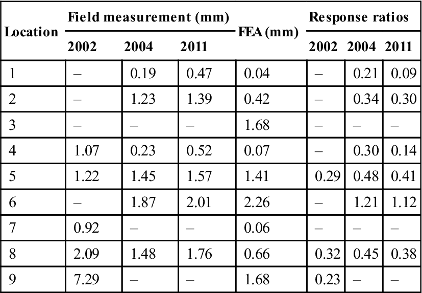
Table 6.9
Response ratios of static deflections from LC3
| Location | Field measurement (mm) | FEA (mm) | Response ratios | ||||
| 2002 | 2004 | 2011 | 2002 | 2004 | 2011 | ||
| 1 | – | 0.67 | 1.59 | 0.67 | – | 1.0 | 0.42 |
| 2 | – | 2.57 | 2.97 | 2.67 | – | 1.04 | 0.90 |
| 3 | – | – | – | 0.78 | – | – | – |
| 4 | 1.66 | 0.79 | 1.77 | 0.94 | – | 1.19 | 0.53 |
| 5 | 4.70 | 3.24 | 3.46 | 3.10 | 0.60 | 0.87 | 0.82 |
| 6 | – | 0.68 | 1.79 | 0.97 | – | 1.43 | 0.54 |
| 7 | 1.21 | – | – | 0.75 | – | 0.62 | – |
| 8 | 3.67 | 3.26 | 3.52 | 2.61 | 0.71 | 0.80 | 0.74 |
| 9 | 1.69 | – | – | 0.69 | 0.41 | – | – |
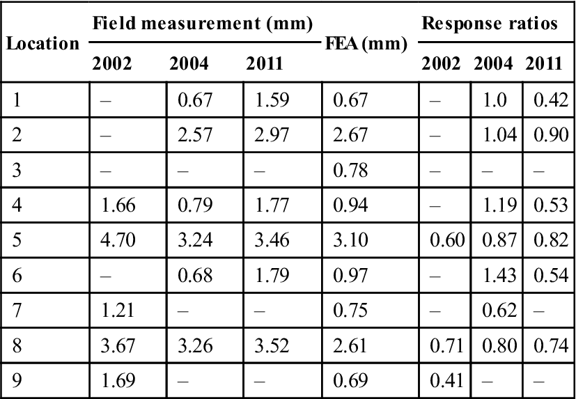
Table 6.10
Response ratios of static deflections from LC4
| Location | Field measurement (mm) | FEA (mm) | Response ratios | ||||
| 2002 | 2004 | 2011 | 2002 | 2004 | 2011 | ||
| 1 | – | 1.42 | 2.22 | 1.67 | – | 1.17 | 0.75 |
| 2 | – | 2.77 | 3.21 | 1.02 | – | 0.37 | 0.32 |
| 3 | – | – | – | 1.71 | – | – | – |
| 4 | 6.95 | 2.18 | 2.56 | 2.36 | 0.34 | 1.08 | 0.92 |
| 5 | 6.87 | 6.48 | 7.04 | 5.32 | 0.27 | 0.38 | 0.35 |
| 6 | – | 2.14 | 2.64 | 2.32 | – | 1.08 | 0.88 |
| 7 | 4.87 | – | – | 1.85 | 0.38 | – | – |
| 8 | 4.01 | 3.29 | 3.63 | 0.99 | 0.25 | 0.30 | 0.27 |
| 9 | 6.31 | – | – | 1.74 | 0.28 | – | – |
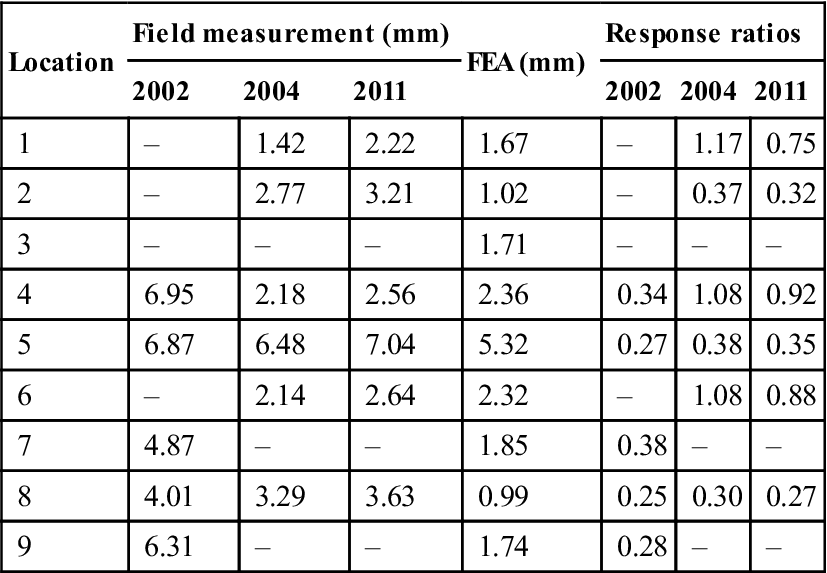
Table 6.11
Response ratios of static strains from LC1
| Location | Field measurement (με) | FEA (με) | Response ratios | ||||
| 2002 | 2004 | 2011 | 2002 | 2004 | 2011 | ||
| 1 | – | 9.2 | 27.3 | 59.6 | – | 6.48 | 2.18 |
| 2 | – | 19.3 | 15.8 | 18.3 | – | 0.95 | 1.16 |
| 3 | – | 5.4 | 10.7 | 3.2 | – | 0.59 | 0.30 |
| 4 | – | 51.2 | 54.3 | 101.7 | – | 1.99 | 1.87 |
| 5 | 41.1 | 37.8 | 31.4 | 26.8 | 0.65 | 0.71 | 0.85 |
| 6 | – | 3.6 | 7.5 | 6.5 | – | 1.81 | 0.87 |
| 7 | 162.5 | 26.7 | 67.0 | 76.1 | 0.47 | 2.85 | 1.14 |
| 8 | – | 24.9 | 28.1 | 21.8 | – | 0.88 | 0.78 |
| 9 | 4.4 | 6.3 | 11.2 | 13.1 | 2.98 | 2.08 | 1.17 |
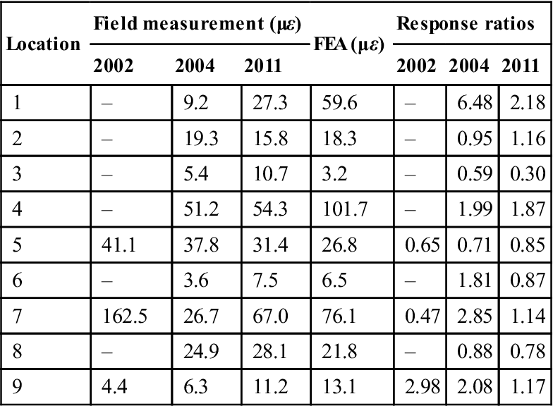
Table 6.12
Response ratios of static strains from LC2
| Location | Field measurement (με) | FEA (με) | Response ratios | ||||
| 2002 | 2004 | 2011 | 2002 | 2004 | 2011 | ||
| 1 | – | 9.8 | 9.5 | 4.1 | – | 0.42 | 0.43 |
| 2 | – | 19.4 | 19.1 | 19.3 | – | 0.99 | 1.01 |
| 3 | – | 1.8 | 35.0 | 71.3 | – | 39.61 | 2.03 |
| 4 | – | 6.3 | 11.7 | 7.3 | – | 1.56 | 0.62 |
| 5 | 35.6 | 30.4 | 31.6 | 25.6 | 0.72 | 0.84 | 0.81 |
| 6 | – | 56.7 | 55.0 | 99.7 | – | 1.76 | 1.81 |
| 7 | 1.3 | 6.6 | 12.9 | 14.9 | – | 2.26 | 1.16 |
| 8 | – | 23.2 | 27.2 | 19.8 | – | 0.85 | 0.73 |
| 9 | 194.3 | 39.2 | 52.3 | 58.3 | 0.30 | 1.49 | 1.11 |
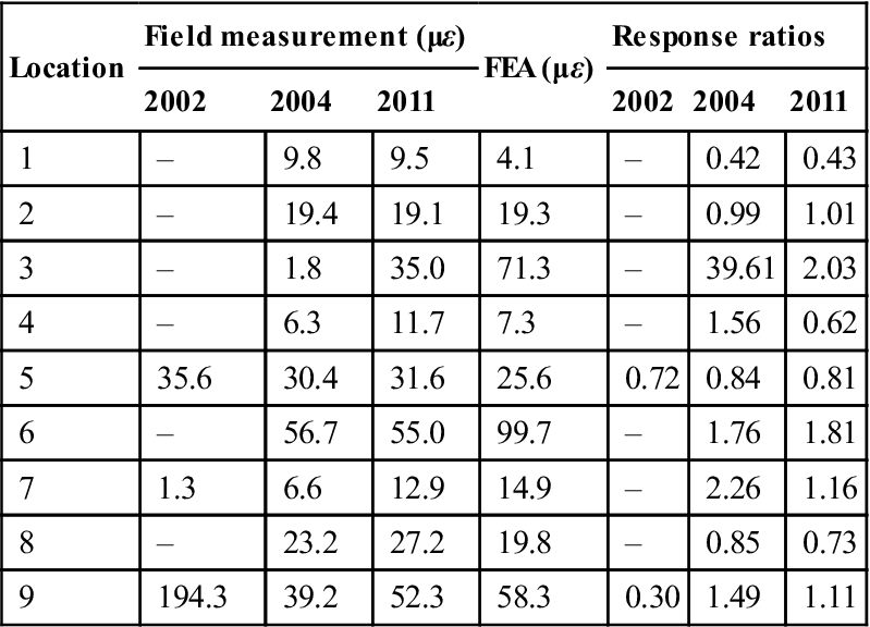
Table 6.13
Response ratios of static strains from LC3
| Location | Field measurement (με) | FEA (με) | Response ratios | ||||
| 2002 | 2004 | 2011 | 2002 | 2004 | 2011 | ||
| 1 | – | 24.9 | 31.0 | 24.3 | – | 0.98 | 0.78 |
| 2 | – | 26.6 | 38.9 | 31.3 | – | 1.18 | 0.80 |
| 3 | – | 16.2 | 32.1 | 38.2 | – | 2.36 | 1.19 |
| 4 | – | 18.9 | 37.0 | 42.9 | – | 2.27 | 1.16 |
| 5 | 91.9 | 76.7 | 81.6 | 60.4 | 0.66 | 0.79 | 0.74 |
| 6 | – | 11.9 | 33.8 | 46.3 | – | 3.89 | 1.37 |
| 7 | 44.7 | 21.7 | 55.6 | 31.9 | 0.71 | 1.47 | 0.57 |
| 8 | – | 49.9 | 58.8 | 40.4 | – | 0.81 | 0.69 |
| 9 | 45.1 | 23.5 | 36.6 | 27.1 | 0.60 | 1.15 | 0.74 |
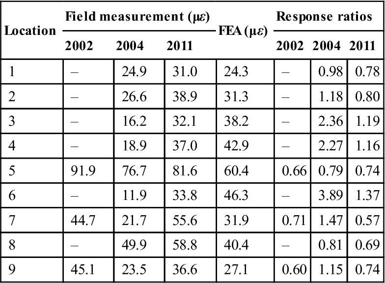
Table 6.14
Response ratios of static strains from LC4
| Location | Field measurement (με) | FEA (με) | Response ratios | ||||
| 2002 | 2004 | 2011 | 2002 | 2004 | 2011 | ||
| 1 | – | 15.8 | 41.2 | 63.6 | – | 4.03 | 1.54 |
| 2 | – | 36.4 | 46.1 | 37.6 | – | 1.03 | 0.82 |
| 3 | – | 4.3 | 47.4 | 74.5 | – | 17.33 | 1.57 |
| 4 | – | 51.7 | 58.3 | 108.9 | – | 2.11 | 1.87 |
| 5 | 90.3 | 70.2 | 76.3 | 52.5 | 0.58 | 0.75 | 0.69 |
| 6 | – | 57.9 | 66.3 | 106.3 | – | 1.84 | 1.60 |
| 7 | 197.5 | 28.7 | 82.0 | 90.9 | 0.46 | 3.17 | 1.11 |
| 8 | – | 51.1 | 64.5 | 41.6 | – | 0.81 | 0.64 |
| 9 | 200.6 | 39.6 | 66.7 | 71.4 | 0.36 | 1.80 | 1.07 |
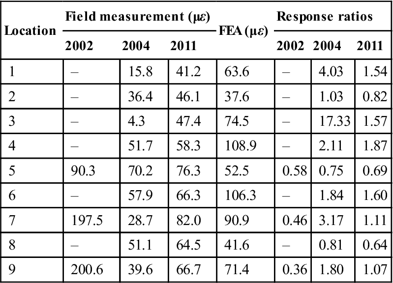
Finally, the capacity rating of the FRP bridge in 2002, 2004, and 2011 was calculated using the minimum RFs and stress modification coefficients ks based on the tables discussed above. The minimum RF could be obtained from Table 6.6 directly. According to Equation [6.27], the minimum ks should be the product of the minimum response ratios and impact factor ratios, defined as (1+ical)/(1+imea). The minimum response ratios could be obtained from Tables 6.7 to 6.14. The impact factor ratio defined above should not exceed 1.0. Once the minimum RF and ks were obtained, the capacity rating could be conducted according to Equation [6.24]. The results are summarized in Table 6.15.
Table 6.15
| Year | Minimum RF | Minimum ks | Capacity rating | ||
| Response ratio | Impact factor ratio | ||||
| Deflection | Strain | ||||
| 2002 | 8.78 | 0.23 | 0.30 | 0.77 | 1.56 × Pr |
| 2004 | 8.78 | 0.20 | 0.32 | 1.00 | 1.76 × Pr |
| 2011 | 8.78 | 0.19 | 0.30 | 1.00 | 1.66 × Pr |
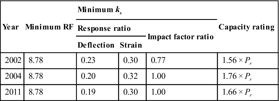
The capacity rating for the FRP bridge turned out to be DB24.00 (total weight of 432.645 kN) in 2002, DB24.99 (total weight of 441.10 kN) in 2004, and DB23.88 (total weight of 429.39 kN) in 2011. There was little difference in the capacity rating between 2002, 2004, and 2011. Since the rated capacity of the FRP superstructure in this study was close to the design live load, it might be concluded that the FRP superstructure had good in-service performance in the past 9 years.
6.5 Construction time and costs
The construction of the FRP superstructure was quite efficient in time and labor. It was completed in only 8 hours, with a crane and four workers on the construction site. If the fabrication period in the factory was also included, the FRP superstructure was completed in 30 days. The total construction cost of the bridge was $140 050. The total cost covered both the FRP superstructure ($84 030) and concrete abutments ($56 020). The estimated construction cost of the FRP sandwich superstructure with corrugated cores was $1750/m2, while an estimated cost for a concrete bridge was $1400/m2. The construction cost of the FRP superstructure was 25% higher than that for conventional concrete bridges. With further design optimization and efficient manufacturing methods, the costs of bridges with FRP superstructures could be decreased in future applications. Therefore, bridges with FRP superstructures like the one in this study may be able to compete with those with conventional materials, especially when shorter on-site construction time and less required maintenance are considered in the future.

6.6 Conclusions
The design, fabrication, construction, and in-service structural performance of an FRP superstructure for ABC are demonstrated in this chapter. Based on the previous discussions, the following conclusions can be drawn:
1. The FRP sandwich superstructure discussed can effectively meet the requirements for stiffness and strength. Connection details are also presented and found working well.
2. The preliminary design approach explained here is effective for estimating the behavior of the FRP sandwich superstructure. It allows the preliminary design to be performed without applying more complicated methods like FEA.
3. The dynamic effects in this study are of less significance. The dynamic responses are close to the static ones, partly due to the difference between the natural frequency of the FRP superstructure and the forced frequency from the passing truck.
4. The construction of the bridge with the FRP superstructure is very efficient in time and labor. The proposed system is considered as a highly competitive short-span bridge alternative for ABC.
5. In the FRP superstructure, there is no corrosion, or damage such as local tearing of the fibers and resin matrix, around the connections of the FRP components. This observation could lead to reduced maintenance strategies compared to other superstructures with conventional materials. However, some maintenance about the wearing surface might be required in the future.
6. To date, a key issue is the lack of design standards relevant to long-term performance of bridges with FRP superstructures. The results presented in this chapter should provide baseline data for future capacity rating assessment, and serve as a part of the long-term performance monitoring of the FRP superstructure.
6.7 Acknowledgment
The work presented in this chapter was partially sponsored by National Science Foundation under Grant No. 0550899 awarded to the third author. The assistance and support from the Korea Land Corporation, Won-chang Technology Ltd, and Seong-won Construction Ltd are also gratefully acknowledged.