
The use of carbon fiber-reinforced polymer (CFRP) composites for cable-stayed bridges
W. Xiong, Southeast University, China
C.S. Cai, Louisiana State University, USA
R.C. Xiao, Tongji University, China
Abstract:
This chapter introduces fiber-reinforced polymer (FRP) applications for cable-stayed bridges with carbon fiber-reinforced polymer (CFRP) stay cables, hybrid stay cables, and/or a CFRP bridge deck. For each of these CFRP components, key design parameters and design strategies are determined and the appropriate value of each key design parameter is suggested. Using the suggested parameter values, six types of cable-stayed bridges with a main span length of 1400 m are selected and modeled with the finite element method, through which the procedures of designing composite cable-stayed bridges with CFRP components are presented in detail. From a mechanical-behavior viewpoint (static and dynamic) a comparative study of composite cable-stayed bridges with various CFRP components is performed through numerical simulation. The economic aspects of each type of cable-stayed bridge is also comparatively studied with respect to material prices. With their high strength-to-weight ratio, and other advantages of CFRP materials, it is proven in this study that the use of CFRP components in super-long-span cable-stayed bridges is feasible, and that these types of composite cable-stayed bridges could become excellent alternatives to steel cable-stayed bridges where super-long spans are desired.
Key words
cable-stayed bridges; CFRP bridge deck; CFRP stay cables; design theory; hybrid stay cables
8.1 Introduction
Fiber-reinforced polymers (FRPs) materials are increasingly being used in engineering bridges with long spans (Meier, 1987; Schurter and Meier, 1996; Saadatmanesh and Ehsani, 1998; Rabinovitch and Frostig, 2003; Schilde and Seim, 2007). The use of cable-stayed bridges with FRP composite stay cables (including hybrid stay cables) and/or FRP composite bridge decks has become more popular. With their light weight and superior strength, FRP composite materials can be used to improve load-carrying efficiency and to extend the span length of cable-stayed bridges over 1000 m. The excellent durability and corrosion resistant behavior of FRP composite materials make FRP composite cable-stayed bridges suitable in aggressive environments, such as crossing seawater. These features of FRP materials may make them very attractive and appropriate when designing cable-stayed bridges with super-long spans (Meier, 1987). Due to strength considerations, carbon fiber-reinforced polymers (CFRPs) become the best choice of FRP materials, with the widest range of practical applications, which will be discussed in the following sections (Noisternig and Jungwirth, 1998; Noisternig, 2000).
8.2 Design of carbon fiber-reinforced polymer (CFRP) bridge decks
A number of commercial CFRP bridge decks are available in the market today; however, how to mechanically design a good CFRP bridge deck is still an unsolved issue, especially in making the most of the CFRP’s advantages. In this chapter, two design theories of CFRP bridge decks, strength criterion design and stiffness criterion design, are proposed in detail. It can be concluded that the buckling and local stiffness need to be carefully designed when using CFRP materials for bridge decks.
8.2.1 Strength criterion design
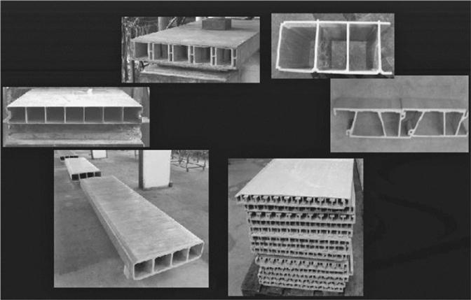
The majority of CFRP bridge-deck systems generally use carbon-reinforcing fibers set in a polyester, epoxy, or vinyl ester resin matrix, resulting in a lightweight decking system that can be rapidly erected while providing excellent long-term durability. Typical CFRP bridge-deck systems consist of two principal types:
• pultruded tubes that are bonded together with an adhesive and honeycomb; or
• sandwich core systems that are laid-up by hand or use vacuum-assisted resin transfer molding techniques.
Several examples of CFRP bridge-deck systems are shown in Fig. 8.1. Each deck system is usually factory assembled into panels that are sized appropriately for shipment to site. The panels can then be erected and bonded together in situ using high performance adhesives.
A number of commercial CFRP bridge decks are already available in the market. However, the mechanical design of a good CFRP bridge deck is still a matter of debate (Hayes et al., 2000; Cai et al., 2009). According to ACI (2004), the ultimate strength of CFRP materials applied on the bridge deck (2700 MPa for tension and 1440 MPa for compression) is much higher than that of common steel materials (345 MPa for both tension and compression), which is one of the significant advantages of CFRP materials. However, usually this high ultimate strength will not be fully utilized, because the bridge deck needs to have a proper safety margin against sudden material damage or failure (or controlled by stiffness). Also, there is no early warning before sudden material damage or failure, due to the linear elastic behavior of CFRP materials and lack of yielding point. For these reasons, an allowable flexural stress of CFRP materials, which is less than the ultimate strength, needs to be specified when designing CFRP bridge decks. This allowable flexural stress can be seen as one of the most significant mechanical parameters of a CFRP bridge deck, determining the whole mechanical performance of the deck during the design process. In view of this, a safety factor for a bridge deck was used to calculate the allowable flexural stress of CFRP materials from their ultimate strength. Hereafter, the conditions under which the allowable flexural stress is reached are designated as ‘design conditions,’ and the conditions under which the ultimate strength of materials is reached are referred to as ‘ultimate conditions’ of materials.
A practical and user-friendly approach was used in the present study to determine a proper value for the safety factor of CFRP materials applied in bridge deck (Xiong et al., 2011). Three typical expressions for the safety factor are:
[8.1]
where kD, kL, and kE = safety factors defined by deformation, load-carrying capacity, and deformation energy, respectively;
Du, Lu, and Eu = deformation, load-carrying capacity, and deformation energy in the ultimate condition of materials, respectively; and
Dd, Ld, and Ed = deformation, load-carrying capacity, and deformation energy in the design condition of materials, respectively.
It should be pointed out that all the different expressions of the safety factor (kD, kL, and kE) need to be calculated based on the same design and ultimate conditions of materials. For steel materials, the allowable flexural stress for bridge structure/component design (design condition) is typically set as 0.55Fy (where Fy is the yield strength, also the theoretical ultimate strength of steel materials in design or ultimate condition) to ensure adequate safety against the catastrophic failure of materials. Then, in the given design and ultimate conditions of steel materials, kD can be firstly set as 4.00 based on the common ductility ratio in steel structure design (usually 4~6). The other safety factors, kL and kE, of steel materials can be easily calculated as 1.82 and 11.24 respectively, based on the pre-set value of kD (4.00), Equation [8.1], and the idealized bilinear relationship of the stress–strain curve (Xiong et al.,2011).
If both deformation and load-carrying capacity are considered, a new expression for the safety factor can be established as:
[8.2]
where: kDL = safety factor defined by both deformation and load-carrying capacity; m and n = weight coefficients, both of which are equal to 1.0 in the present study. For steel materials, typically kDL = 7.28 according to Equation [8.2].
As with steel design, the design safety level of CFRP bridge decks can also be developed or adjusted using a proper safety factor value. A safety level of design similar to steel materials is proposed here for CFRP materials before more appropriate strategies are available. This is the basic idea behind the proposed strategy specifying an allowable flexural stress for CFRP materials applied in bridge decks. Assuming one of the four safety factors kD, kL, kE, and kDL of CFRP materials is identical to that of steel materials, the other three values, as shown in Table 8.1, can be determined using Equations [8.1] and [8.2]. Due to the linear elastic behavior of CFRP materials and lack of yielding point, the calculated kD is the same as kL, and kE is the same as kDL for CFRP materials.
Table 8.1
Safety factor of CFRP materials
| Safety factor | CFRP | Steel | |
| Case (1) | kD | 4.00 | 4.00 |
| kD is identical to that of steel materials | kL | 4.00 | 1.82 |
| kE | 16.00 | 11.24 | |
| kDL | 16.00 | 7.28 | |
| Case (2) | kD | 1.82 | 4.00 |
| kL is identical to that of steel materials | kL | 1.82 | 1.82 |
| kE | 3.31 | 11.24 | |
| kDL | 3.31 | 7.28 | |
| Case(3) | kD | 3.35 | 4.00 |
| kE is identical to that of steel materials | kL | 3.35 | 1.82 |
| kE | 11.24 | 11.24 | |
| kDL | 11.24 | 7.28 | |
| Case (4) | kD | 2.70 | 4.00 |
| kDL is identical to that of steel materials | kL | 2.70 | 1.82 |
| kE | 7.28 | 11.24 | |
| kDL | 7.28 | 7.28 |

As can be seen from case (1) in Table 8.1, if the deformation safety factor of CFRP materials is taken to be the same as that of steel materials, i.e., kD = 4.00, the values of the other three safety factors such as kL will be much larger than those of steel materials, indicating that the material strength will not be fully used. In contrast, if the safety factor of the load-carrying capacity of CFRP materials is set at the same level as steel materials, i.e., kL = 1.82 as in case (2), the values of the other three safety factors such as kD will be much lower than those of steel materials, indicating insufficient ductility and possible catastrophic failure of CFRP materials.
If kE and kDL are given the same values as those of steel materials, i.e., kE = 11.24 in case (3) or kDL = 7.28 in case (4), the other three values for the safety factor of CFRP materials will be similar to those of steel materials. In other words, the safety level of designing CFRP materials using kE = 11.24 or kDL = 7.28 will be similar to that in designing steel materials. Therefore, they could be used in practical applications before further information on CFRP performance becomes available and design strategies are established. In the present study, the safety factor values resulting from kDL = 7.28 in case (4) were selected for the design of a CFRP deck in the following study resulting in a safety factor for load-carrying capacity kL = 2.7. This kL value of 2.7 is similar to the 2.5 used for steel stay cables. As a result, the allowable flexural stress of CFRP deck materials was calculated as 2700/2.70 = 1000 MPa for tension and 1440/2.70 = 533.33 MPa for compression.
It can be clearly seen that the allowable flexural stress of CFRP materials can be set much higher than for steel materials. Therefore, by following the design procedure of traditional steel bridge decks, the strength requirement in designing CFRP bridge decks could be easily satisfied.
8.2.2 Stiffness criterion design
Besides the strength requirement however, the buckling and deflection requirements of CFRP bridge decks, referred to as ‘buckling and local stiffness requirement,’ should also be satisfied in the design process. Due to the lower elastic modulus of CFRP materials, the buckling of a CFRP bridge deck could be a critical problem in design. Also, the deflection of a CFRP bridge deck subjected to vehicle loads could be larger than that of a steel bridge deck of equal thickness. Excessive deflection will not only accelerate the deterioration of bridge-deck pavement but will also affect ride quality and bridge-deck durability. Therefore, greater attention needs to be paid to buckling and local stiffness when designing CFRP bridge decks.
In the present study, to ensure adequate buckling capacity and local stiffness of CFRP bridge decks, the stiffness was designed to be equal to that of the reference model of traditional steel cable-stayed bridges, since there are no corresponding stiffness design guidelines for CFRP bridge decks. This practice was based on an assumption that the design for the steel bridge deck of traditional cable-stayed bridges completely satisfies the buckling and local stiffness requirements. For a rectangular solid cross-section of a CFRP bridge deck (or equivalently solid, because hollowed sandwich panels are commonly used for CFRP bridge decks), its thickness can be easily calculated based on the required local stiffness of the bridge deck:
[8.3]
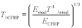 [8.3]
[8.3]where: ThCFRP and Thsteel = thicknesses of the CFRP and steel bridge decks, respectively; and ECFRP and Esteel = elastic modulus of the CFRP and steel materials, respectively.
For the buckling stiffness case, the thickness of a CFRP bridge deck can also be calculated using the same methodology. From a construction viewpoint, bonding issues between CFRP deck and steel girder are also very important. The materials used to reliably bond CFRP deck and steel girder could be considered the same as when using CFRP laminates to strengthen steel girders. Many related studies have been conducted and reported to ensure adequate adhesive capacity between CFRP laminates and steel girders (Sen et al., 2001; Matta, 2003; Schnerch et al., 2004, 2005; Colombi and Poggi, 2006; Rizkalla et al., 2008; Zhao, 2008). Zhao and Zhang (2007) also gave a state-of-the-art review on the CFRP strengthened steel structures including bond test methods, failure modes in a CFRP bonded steel system, bond strength, and bond-slip relationships. All the studies proved that appropriate bond materials and techniques between the steel and CFRP materials do exist (for example, epoxy resin) and can be reliably applied to strengthening structures. While it is reasonable to believe that a reliable bond between a CFRP deck and a steel girder should also be obtained using the same or similar bond materials and techniques as used for strengthening structures, the bond issue of CFRP bridge-deck design may deserve further research.
Based on the analysis above, the buckling and local stiffness needs to be carefully considered if using CFRP materials for bridge decks. The strength requirement of designing CFRP bridge decks could be easily satisfied, and it is believed that the connection between CFRP deck and steel girder can be also reliably constructed using the same bonding materials and techniques used for strengthening engineering.
8.3 Design of CFRP stay cables
With light weight and superior strength, the applications of CFRP stay cables should highly improve the load-carrying efficiency and extend the span length of cable-stayed bridges to over 1000 m. Herein, the key design parameter for CFRP stay cables and their appropriate span lengths were investigated in order to assure a logical design. A conclusion can be drawn that 1400 m could be a good starting point to apply CFRP stay cables in cable-stayed bridges if considering an obvious advantage in stiffness.
8.3.1 Key design parameter for CFRP stay cables
CFRP materials, being stronger and lighter, can be used as new materials for stay cables, improving their load-carrying efficiency and effectively extending the span length of cable-stayed bridges to over 1000 m. Since the stiffness, weight, and ultimate strength of a stay cable largely depends on its cross-sectional area, in the present study the cross-sectional area of stay cables is determined as the key design parameter for CFRP stay cables. A stay cable design ensures adequate allowable strength for the stay cables if their design forces are given. Therefore, to obtain an appropriate cross-sectional area, the allowable axial stress of CFRP stay cables should firstly be determined using the following expression (Xiong et al., 2012):
[8.4]
where:
fCFRP = allowable axial stress of the CFRP stay cables (working stress);
uCFRP = ultimate strength (stress) of the CFRP stay cables; and
kS = safety factor.
According to Xiong et al. (2011, 2012), in the present study, uCFRP and kS were set as 2550 MPa and 2.50, respectively, resulting in:
Then the appropriate cross-sectional areas of CFRP stay cables can be obtained as:
where:
ACFRP = cross-sectional area of the CFRP stay cable; and
F = unfactored design force of the stay cable.
For a given cable force the cross-sectional areas of CFRP stay cables can be calculated from the steel stay cables in traditional cable-stayed bridges using the equivalent strength criterion:
where Asteel and fsteel are cross-sectional area and allowable axial stress, respectively, of steel stay cables used in traditional cable-stayed bridges.
8.3.2 Appropriate span lengths of CFRP stay cables
As is known, the equivalent stiffness of stay cables determined by cross-sectional area is usually seen as the judging criterion in determining appropriate span lengths. To better understand the effect of equivalent stiffness on the appropriate span lengths of CFRP stay cables, four mechanical parameters (equivalent stiffness and three other related parameters, see Table 8.2) were theoretically investigated through a parametric study by varying the ‘cable span lengths’ (horizontally projected length of stay cables) from 50 to 25 000 m using analytical models (see Table 8.3). These four mechanical parameters enable the equivalent stiffness of stay cables to be comprehensively described, directly or indirectly, and all of them are the key study objectives for span length studies in literature (O’Brien and Francis, 1964; Ernst, 1965; Irvine, 1981; Ahmadi-Kashani and Bell, 1988; Gimsing, 1997; Freire et al., 2006). Based on the results of this parametric study the appropriate span lengths of CFRP stay cables can be recommended.
Table 8.2
Mechanical parameters and analytical solutions (Ernst, 1965; Gimsing, 1997)
| Mechanical parameters | Analytical solutions |
| 1. Equivalent stiffness | 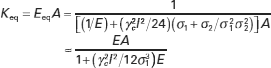 |
| 2. Load-carrying efficiency (real gradient of stay cables) | 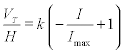 |
| 3. Cable sag effects | 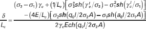 |
| 4. Self-weight stress | 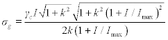 |
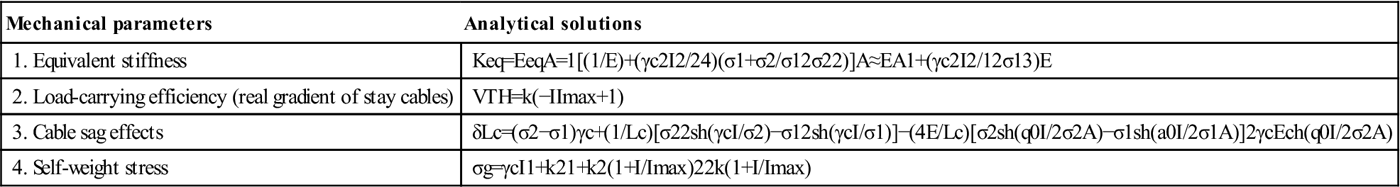
Notes: Keq = equivalent stiffness of stay cables; Eeq = equivalent elasticity modulus; E = elasticity modulus; A = area of the cross-section of stay cables; γc = q0/A = density of stay cables; q0 = distributed loads (uniform gravity loads) per unit length of stay cables; I = horizontally projected length of stay cables; σ1 and σ2 = stress of stay cable in two load conditions (usually dead load and dead + live load conditions), respectively; VT= vertical component of the cable force in the actual curved cable; H = horizontal component of the cable force in the actual curved cable; h = vertically projected length of stay cables; k = h/I; Imax = ultimate horizontally projected length of stay cables; δ/Lc = cable sag effect; Lc = chord length of stay cables; ch( ) = the function of hyperbolic cosine; and σg = self-weight stress of stay cables.The detailed derivations of these equations are not presented here and can be found in the literature (Ernst, 1965; Gimsing, 1997).
Table 8.3
Design parameters of analytical models (CFRP stay cables)
| Design parameters | Values | ||
| Nominal gradient of stay cables (k = h/I) | 0.3 | 0.4 | 0.5 |
| Cable span length (m) | 50~30 000 | 50~30 000 | 50~30 000 |
| Vertically projected length of stay cables (m) | 15~9000 | 20~12000 | 25~15 000 |
| Area (m2) | 0.00638 | ||
| Design stay cable (N) | 5.102E + 6 | ||
| Elasticity modulus (N/m2) | 1.37E + 11 | ||
| Density (kg/m3) | 1.60E + 03 | ||
| Breaking strength (MPa) | 1.02E + 03 | ||
| Safety factor | 2.50 |
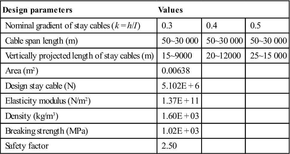
Figure 8.2a–8.2d shows the performance of CFRP stay cables with regard to the investigated mechanical parameters when varying the cable span lengths from 0 to 30 000 m. The numbers 0.3, 0.4, and 0.5 in the figures denote the nominal gradients of stay cables (k) for the investigated cable models. Firstly, Fig. 8.2a–8.2d shows that the reduction or deterioration of mechanical behavior representing the equivalent stiffness of stay cables becomes more and more obvious when the cable span length increases from 0 to 30 000 m. Furthermore, 5000 m could be a significant cable span length after which all the investigated mechanical behaviors deteriorate more rapidly and suddenly than before, or already have an unacceptable reduction. Indeed, almost a 20% reduction in equivalent stiffness, 18% reduction in load-carrying efficiency, 0.0028 cable sag effects (about 70 m cable sagging), and 10% as the ratio of self-weight stress to breaking strength are observed at the 5000 m point in Fig. 8.2a–8.2d, respectively. By comparison Fig. 8.3 demonstrates that steel stay cables (area = 0.00974 m2, design stay cable force = 5102 kN, elasticity modulus = 200 GPa, density = 7850 kg/m3, yield strength = 668 MPa, and safety factor = 2.50 (ACI 2004)) show an obvious advantage in stiffness before the cable span length reaches 1400 m; however, beyond this length CFRP stay cables have the advantage. In other words, 1400 m could be a suitable starting point for CFRP stay cables in cable-stayed bridges. Therefore, in the present study, 1400~5000 m was determined as an appropriate span length of CFRP stay cables from a stiffness viewpoint. Additionally, 30 000 m could be considered as the maximum span length for pure CFRP stay cables as beyond this span length almost all the stiffness has been lost.


8.4 Design of CFRP–steel hybrid stay cables
Directly replacing steel stay cables with CFRP stay cables could result in an increase in displacement under loading, which is actually the main obstacle to the development of such bridges with CFRP stay cables. Hybrid stay cables using CFRP and steel materials are a novel concept in applying CFRP materials to bridge engineering (Xiong et al., 2011, 2012). The basic idea of this hybrid concept is to create a new structure incorporating the advantages of both materials. There are several possible methods to form the hybrid stay cables. One of the most straightforward ways is to simultaneously install both CFRP stay cables and steel stay cables at the same location as shown in Fig. 8.4. By doing this, CFRP stay cables retain all the advantages of CFRP materials, such as their light weight and high strength, while steel stay cables increase the axial stiffness and reduce the total cost of the materials. The steel and CFRP cables can be installed separately in order to control the forces in each cable component.

Due to the different roles played by these two materials, the material proportion of the hybrid stay cables is expected to be a principal factor affecting the behavior and cost of the stay cable. For this reason, in the present study, the ratio of the CFRP section area to the entire section area, ρ = ACFRP/Asteel + CFRP, is determined as the key design parameter for the hybrid stay cables. By adjusting the initial cable forces of both the steel and CFRP components, the possible effects of the differential elastic modulus of the two materials on the composite strength calculation can be resolved. It should be pointed out that the present study only aims at the mechanical or economical behavior of the hybrid stay cables without considering construction-related details, which will be the topic of a separate study.
The analysis conducted by the authors indicated the following:
cable span lengths 0~700 m – pure steel stay cables are more appropriate;
cable span lengths 1400~5000 m – pure CFRP stay cables are more appropriate;
cable span lengths 700~1400 m – combined application of steel and CFRP stay cables may be more appropriate.
As a result, a type of hybrid stay cable system was proposed in the present study for cable-stayed bridges with cable span lengths of 700~1400 m. Through a rational design (see the details later), the hybrid stay cable system can be a good alternative to the traditional pure steel stay cables or pure CFRP stay cables in this particular span length range. In other words, this span length range, i.e., 1400~2800 m for main span lengths of cable-stayed bridges, or 700~1400 m for the longest cable span lengths, can be regarded as the appropriate application range for the hybrid stay cable system.
8.4.1 Hybrid stay cable system
Also, for this type of hybrid stay cable system, a further increase in the equivalent stiffness could be obtained with a reasonable increase in their safety factor, i.e., increasing the section area of stay cables. It should be noted that this increasing-safety-factor-method may not be the best option for either pure steel or pure CFRP stay cables because it could result in increased weight or higher cost. When building appropriate connections between the steel stay cables and CFRP stay cables during or after construction, the hybrid stay cable can theoretically be regarded as a single cable with a composite section.
As stated earlier, in the present study, the ratio of the section area of CFRP stay cables to the whole cable area, i.e., ρ = ACFRP/(Asteel + ACFRP),was determined as the key design parameter for the hybrid stay cable system. It is easy to understand that this parameter can directly determine almost all the mechanical behaviors of the hybrid stay cables, such as strength, density, elastic modulus, and self-weight.
8.4.2 Analytical study for equivalent stiffness of the hybrid stay cable system
Before the introduction of design strategy (design criteria) an analytical study of the equivalent stiffness of the hybrid stay cable system was carried out. In the present study the equivalent stiffness of the hybrid stay cable system is defined as EeqA:
[8.6]
By assuming that the steel and CFRP stay cables can be pulled separately to achieve a desired force level for the hybrid stay cable system, each section area can be designed as:
[8.7]
[8.8]
where: Asteel and ACFRP = section areas of the steel and CFRP stay cables, respectively; Fsteel and FCFRP = stay cable forces of the steel and CFRP stay cables, respectively; σasteel and σaCFRP = allowable stresses of the steel and CFRP stay cables, respectively; σlsteel and σlCFRP = limit stresses of the steel and CFRP stay cables, respectively; and ηsteel and ηCFRP = safety factors of the steel and CFRP stay cables, respectively.
The density of the hybrid stay cable system can be written as:
[8.9]
where γsteel and γCFRP = densities of the steel and CFRP stay cables, respectively.
By safely assuming the deformation compatibility between the steel and CFRP stay cables after they are installed, the elastic modulus of the hybrid stay cable system can be given as:
[8.10]
where Esteel and ECFRP = elastic modulus of the steel and CFRP stay cables, respectively.
Substituting Equations [8.9] and [8.10] into Equation [8.6], the equivalent stiffness of the hybrid stay cable system can then be described as:
[8.11]
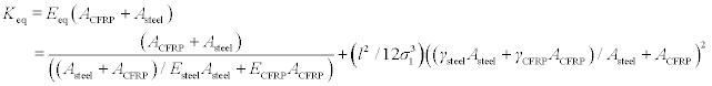 [8.11]
With the definition of ρ = ACFRP/(Asteel + ACFRP), Equation [8.11] can be further transformed into:
[8.12]
 [8.12]
If considering material costs, the ratio of equivalent stiffness to material cost of unit cable length can be calculated as:
[8.13]
 [8.13]
where: ξ = ratio of equivalent stiffness to the material cost of unit cable length; κsteel and kCFRP = costs of unit mass for the steel and CFRP stay cables with the consideration of materials and construction, respectively.
By defining λ = κCFRP/κsteel, Equation [8.13] can be further written as:
[8.14]
 [8.14]
If the total cost for designing stay cables (including materials and construction) of unit cable length is defined as ψ, the section area of the hybrid stay cable system can be designed as:
[8.15]
 [8.15]
[8.16]
[8.17]
Then, substituting Equations [8.16] and [8.17] into Equation [8.12] the equivalent stiffness of the hybrid stay cable system under a given (pre-set) cost ψ (or ‘budget’) can be obtained.
For the convenience of discussion the costs per unit cable length of designing pure steel and pure CFRP stay cables with a safety factor of 2.5 are denoted as ψsteel and ψCFRP respectively and are regarded as the basic costs. Correspondingly, any other possible costs per unit cable length with other safety factors for the hybrid section can be expressed as αψsteel or αψCFRP.
[8.18]
[8.19]
[8.20]
[8.21]
where αψsteel and αψCFRP = α times ψsteel and ψCFRP, respectively.
All the discussed parameters and expressions that describe the characteristics of the equivalent stiffness of stay cables will be used in the following studies.
8.4.3 Design criteria of the hybrid stay cable system
With the consideration of equivalent stiffness and cost, three design criteria for the proposed hybrid stay cable system are introduced in the following sections. Designers can choose one of these criteria in a design process, or other design criteria can be similarly developed.
Design criterion 1: Best equivalent stiffness with a given safety factor
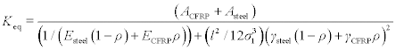
In this design criterion the best equivalent stiffness of stay cables with a given safety factor can be pre-designed by adjusting the area ratio ρ discussed earlier. To better understand the effects of ρ on equivalent stiffness, the equivalent stiffness of stay cables with different safety factors were theoretically investigated through a parametric study. Based on the results of this study, a design methodology for the hybrid stay cable system using this design criterion was recommended in assisting engineers to perform and optimize their designs.
To broaden the possible design conditions in the parametric study, four analytical models of stay cables with different horizontally projected lengths of 400, 700, 1000, and 1300 m respectively, and a constant designed cable gradient of 0.4, were studied mainly using Equations [8.7]–[8.12]. The designed cable force was set as 5102 kN and retained as constant in all the models for convenience of comparison. Also, to verify the proposed methodology for stiffness improvement by increasing the safety factor, eight safety factor values were considered (2.5, 3, 3.5, 4, 4.5, 5, 5.5, and 6), although some of these safety factors are too high in practice. The other geometric and material properties used in the parametric study were kept the same as those applied previously.
Figure 8.5a–8.5d plots the equivalent stiffness of stay cables vs area ratio (0~1.0) obtained with different safety factors (2.5~6) and cable span lengths (400, 700, 1000, and 1300 m) separately. The effects of increasing safety factors on stiffness improvement are clear from these figures. In each figure, the equivalent stiffness of stay cables at 0.0 and 1.0 area ratios represent the two extremes, i.e., pure steel stay cables and pure CFRP stay cables, respectively. The results corresponding to the area ratios between 0.0 and 1.0 are calculated from the hybrid cases. Taking the results with a safety factor of 5 for example, the superior range of the hybrid stay cable system following design criterion 1 is marked by a dashed line between two circles where the equivalent stiffness is higher than that of stay cables with both pure steel (ρ = 0) and pure CFRP (ρ = 1) materials. By repeatedly doing this, all the superior ranges of the hybrid stay cable system (the ranges of area ratio) with regard to different safety factors and cable span lengths can be obtained, and are shown in Fig. 8.6 as a design guide.
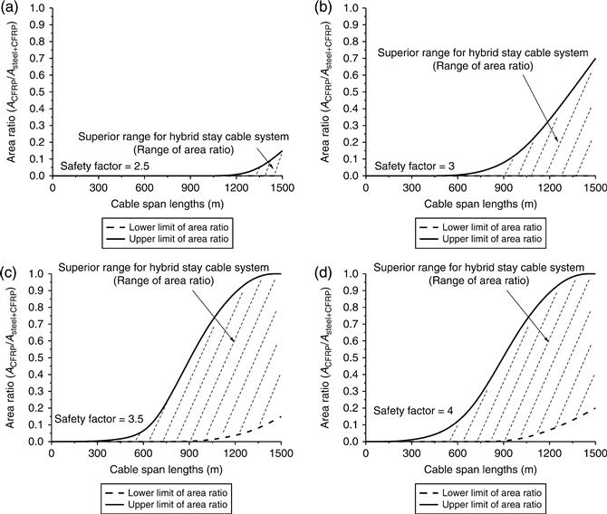
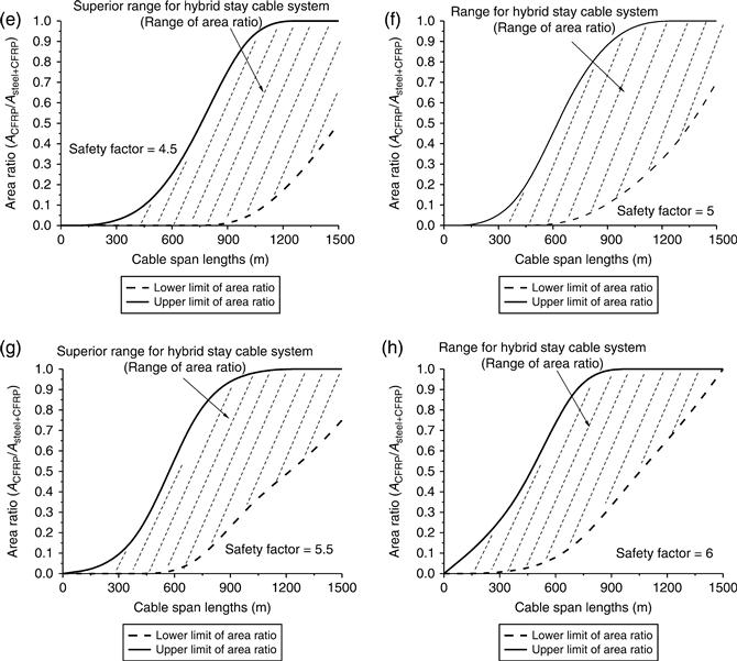
Based on the design guide shown in Fig. 8.6 the hybrid stay cable system can be easily designed using design criterion 1 as follows:
• Step 1: Determining the span lengths of stay cables;
• Step 2: Determining the safety factor used in the cable design;
• Step 3: From the design guide shown in Fig. 8.6, the appropriate area ratio range for the hybrid stay cable system (dashed area) can be selected based on the cable span length and safety factor used in design; furthermore, by using Fig. 8.5, the optimal area ratio corresponding to the highest equivalent stiffness can be obtained;
• Step 4: If no appropriate area ratio can be found based on the design criterion 1, pure steel stay cables can be selected for short cables near the pylon and pure CFRP stay cables for long cables further away from the pylon.
Design criterion 2: Highest ratio of equivalent stiffness to material cost with a given safety factor
In this design criterion the highest ratio of equivalent stiffness to material cost with a given safety factor can be pre-designed by adjusting the area ratio ρ with a given price ratio of CFRP stay cables to steel stay cables. As with design criterion 1, to better understand the effects of ρ on this stiffness-to-cost ratio, a series of parametric studies were carried out in order to obtain a design methodology using design criterion 2.
The analytical models and investigated safety factors for the parametric study are identical to those used for design criterion 1. However, due to the cost factor in this design criterion, different price ratios of the two materials used in the hybrid stay cable system are studied to consider future cost changes. In this study, present prices of CFRP and steel stay cables are assumed as $77.1/kg and $2.9/kg, respectively, resulting in a price ratio of 27:1 (Xiong et al., 2011, 2012) and more price ratios of CFRP stay cables to steel stay cables are also studied, which are 20:1, 15:1, 10:1, 8:1, 5:1, 2:1, and 1:1. For purposes of brevity, only the results of 700 m (Fig. 8.7) and 1000 m (Fig. 8.8) cable span lengths with different price ratios are presented here.
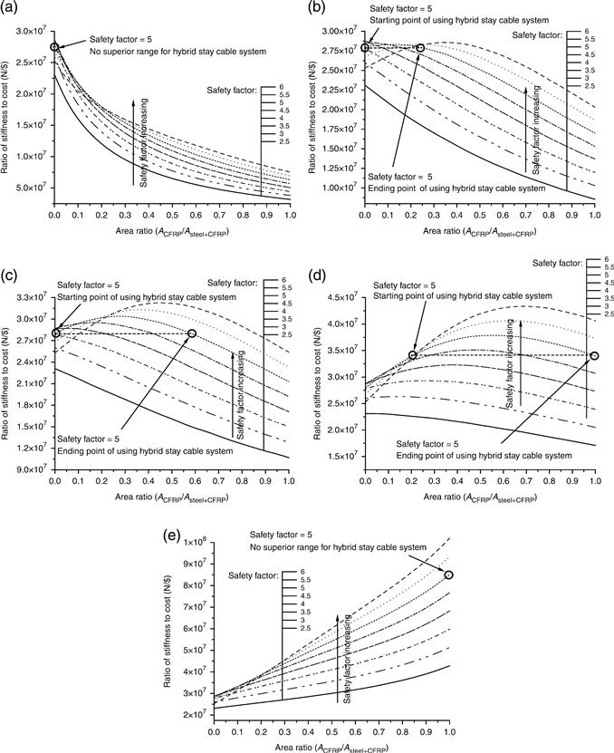

Figures 8.7a–8.7e and 8.8a–8.8e plot the ratio of equivalent stiffness to material cost vs area ratio (0~1.0) obtained with different price ratios (27:1~2:1), safety factors (2.5~6), and cable span lengths (only the 700 and 1000 m) separately. The results demonstrate the beneficial effects of increasing safety factors on stiffness improvement. Following the method used in design criterion 1, the superior ranges of the hybrid stay cable system (the ranges of area ratio) with regard to different price ratios, safety factors, and cable span lengths can also be obtained using design criterion 2, which are shown in Figs 8.9 (price ratio = 15:1) and 8.10 (price ratio = 10:1) as a design guide. Again, the results of other price ratios are not shown here, for reasons of brevity.

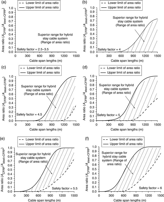
Based on the design guide shown in Figs 8.9 and 8.10, and other figures with more price ratios, the hybrid stay cable system can be easily designed using design criterion 2 as follows:
• Step 1: Determining the span lengths of stay cables;
• Step 2: Checking the recent price ratio of CFRP stay cables to steel stay cables;
• Step 3: Determining the safety factor used in the cable design;
• Step 4: From the design guide shown in Figs 8.9, 8.10, and other figures with more price ratios, the appropriate area ratio range for the hybrid stay cable system (dashed area) can be selected based on the recent price ratio, cable span length, and safety factor used in design; furthermore, by using Figs 8.7 and 8.8, the optimal area ratio corresponding to the highest equivalent stiffness-to-cost ratio can be obtained;
• Step 5: As with criterion 1, if no appropriate area ratio can be found based on design criterion 2, pure steel stay cables can be selected for short cables near the pylon and pure CFRP stay cables for long cables further away from the pylon.
Design criterion 3: Best equivalent stiffness under a given cost
In this design criterion, the best equivalent stiffness of stay cables under a given cost can be pre-designed by adjusting the area ratio ρ under a given price ratio of CFRP stay cables to steel stay cables. The safety factor value used for cables will be automatically determined when the sectional area of each stay cable is set using Equations [8.15]–[8.17] as well as satisfying the strength requirement. As before, a series of parametric studies were carried out in order to obtain a design methodology using design criterion 3.
The analytical models and investigated price ratio for the parametric study are identical to those used for design criteria 1 and 2. However, in addition to the developing price ratio, various given costs (αψsteel and αψCFRP, using Equations [8.18]–[8.21] to define them) prepared for the hybrid stay cable system should also be considered, which are 1ψsteel, 2ψsteel, 5ψsteel, 10ψsteel, 15ψsteel, 1ψCFRP, 2ψCFRP, 5ψCFRP, 10ψCFRP and 15ψCFRP. Once again, only the results of 700 m (Fig. 8.11) and 1000 m (Fig. 8.12) cable span lengths with different price ratios are presented here.
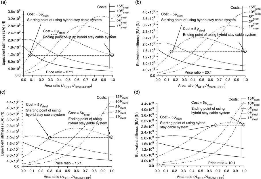
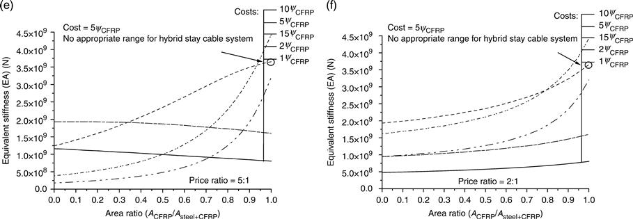
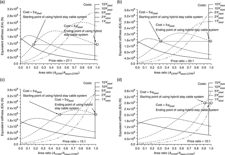
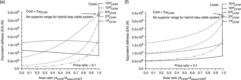
Figures 8.11a–8.11f and 8.12a–8.12f plot the equivalent stiffness of stay cables versus area ratio (0~1.0) obtained with different given costs (1ψsteel~15ψsteel and 1ψCFRP~15ψCFRP), price ratios (27:1~2:1), and cable span lengths (only the 700 m and 1000 m). The reason for switching ψsteel to ψCFRP for the cases of 5:1 and 2:1 price ratios is that in these cases the cost of building CFRP stay cables has been similar to or even less than that of steel stay cables. As with the previous criteria, the dashed line between two circles in each figure shows the superior ranges of the hybrid stay cable system with cost 5ψsteel or 5ψCFRP. The superior ranges of the hybrid stay cable system (the ranges of area ratio) with regard to different costs, price ratios, and cable span lengths can also be obtained using design criterion 3, which are shown in Figs 8.13 (price ratio = 15:1) and 8.14 (price ratio = 10:1) as a design guide. Again, for reasons of brevity, other price ratios are not shown.
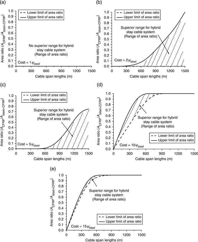
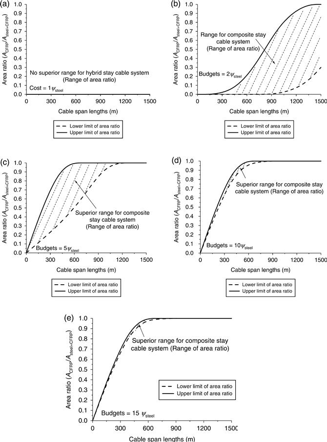
Based on the design guide shown in Figs 8.13, 8.14, and other figures with more price ratios, the hybrid stay cable system can be easily designed using design criterion 3 as follows:
• Step 1: Determining the span lengths of stay cables;
• Step 2: Pre-determining the costs (budget) for the cable design including the materials and construction;
• Step 3: Checking the recent price ratio of CFRP stay cables to steel stay cables;
• Step 4: From the design guide shown in Figs 8.13, 8.14, and other figures with more price ratios, the appropriate area ratio for the hybrid stay cable system (dashed area) can be selected based on the predetermined costs, recent price ratio, and cable span length used in design. Furthermore, by using Figs 8.11 and 8.12, the optimal area ratio corresponding to the highest equivalent stiffness can be obtained for a given cost;
• Step 5: As with criteria 1 and 2, if no appropriate area ratio can be found based on design criterion 3, pure steel stay cables can be selected for short cables near the pylon and pure CFRP stay cables for long cables away from the pylon.
8.4.4 Cable force distribution of the hybrid stay cable system
Once the value of area ratio is determined for the hybrid stay cable system, the cable force distribution between the steel and CFRP stay cables is the next issue. Appropriate cable force distribution affects the stiffness design of stay cables (Ernst, 1965; Ahmadi-Kashani and Bell, 1988; Freire, 2006). Therefore, this study went on to investigate the effects of cable force distribution (defining β = F![]()
![]()
![]()
![]() /(FCFRP + F
/(FCFRP + F![]()
![]()
![]()
![]() ), herein) on the equivalent stiffness of stay cables through a parametric study.
), herein) on the equivalent stiffness of stay cables through a parametric study.
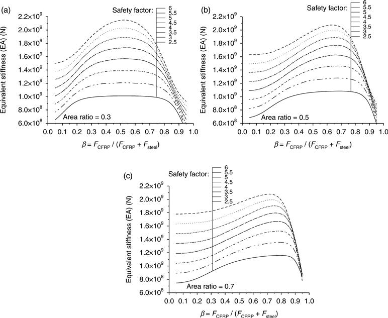
From Figs 8.15 and 8.16 and other figures with more cable span lengths (not shown here for reasons of brevity), the appropriate value of β for each study case usually ranges from 0.4 to 0.7, where the best equivalent stiffness of stay cables can be reached. The variation of the safety factor values has little effect on the β design. It can also be observed that the β value with regard to the equivalent stiffness of stay cables increases with the increase of an area ratio. This can be explained in that CFRP stay cables with higher area ratio need greater cable force applied to maintain their high equivalent stiffness. The final decision as to cable force distribution can only be made when the cable stresses also satisfy the strength requirements. In practice, a good choice of the β value can complement the three design criteria to ensure a high equivalent stiffness for the hybrid stay cable system.

8.5 Case study: 1400 m cable-stayed bridges
From a mechanical-behavior viewpoint (static and dynamic), a comparative study of composite cable-stayed bridges with different CFRP components was performed through numerical simulations. The economical behavior of each type of cable-stayed bridges was also comparatively studied considering the varying material price. With the high strength-to-weight ratio and other advantages of CFRP materials, it was proven that the use of CFRP stay cables and CFRP bridge decks in super longspan cable-stayed bridges is feasible and these types of composite cable-stayed bridges can become an excellent alternative to steel cable-stayed bridges where super longspans are desired.
8.5.1 Bridge models
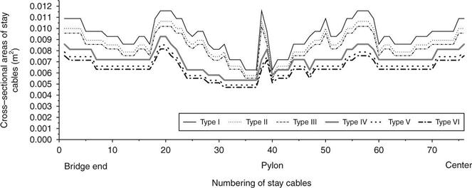
For a comparative study, six selected cable-stayed bridges are shown in Table 8.4 with different combinations of materials. Figure 8.17a shows the span arrangement of the six cable-stayed bridge models with two pylons and double cable planes. The center and side spans were designed as 1400 and 636 m, respectively. For the side span, three intermediate piers were used at a distance of 100 m in order to increase the in-plane flexural rigidity of the bridge. The full height of the A-shape pylon is 357 m, and 287 m of the pylon is above the girder (see Fig. 8.17b). Figure 8.17c shows the cross-section of the girder with a width (Bu) of 32.5 m and a depth (Hw) of 4.5 m. The span-to-width ratio of all the six bridges is 43, larger than the commonly adopted minimum value 40 (Leonhardt and Zellner, 1991). The span-to-depth ratio is 311, which is also larger than those used for other long span cable-stayed bridges, e.g. 285 for the Normandy Bridge (France) and 272 for the Sutong Bridge (China). Four typical cross sections (sections A, B, C, and D) with different properties (Table 8.5) were used in different locations along the span (Fig. 8.17a). The girder is suspended by diagonal stay cables anchored to the girder at 12, 16, and 20 m intervals. The cross-sectional areas of stay cables used in each bridge type are shown in Fig. 8.18. Using design criterion 1, a ρ value of 0.60 for hybrid stay cables was determined as an appropriate value balancing mechanical behavior and cost and was therefore employed for the present case studies. The safety factor of hybrid stay cables was kept as 2.5, remaining consistent with other bridge types for a convenient comparison. It can be seen that a Type I bridge requires the maximum and a Type VI the minimum stay cable areas.
Table 8.4
Definition of the six types of the proposed cable-stayed bridges
| Type | Girder | Bridge deck | Stay cables | Pylons |
| I | Steel | Steel | Steel | Concrete |
| II | Steel | Steel | Hybrid | Concrete |
| III | Steel | Steel | CFRP | Concrete |
| IV | Steel | CFRP | Steel | Concrete |
| V | Steel | CFRP | Hybrid | Concrete |
| VI | Steel | CFRP | CFRP | Concrete |
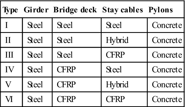
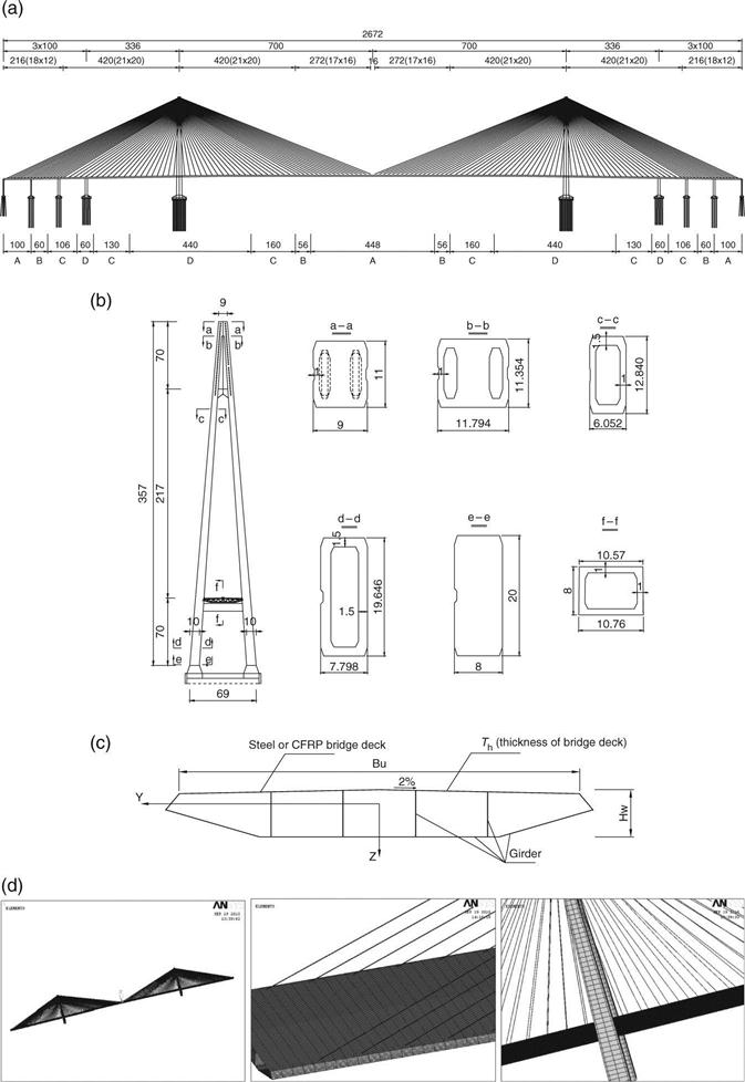
Table 8.5
| Cross-section | Bu (m) | Hw (m) | A (m2) | Th (m) | Iy (m4) | Iz (m4) | J (m4) | |
| Types I, II, and III (Steel bridge deck) | A | 32.5 | 4.5 | 1.688 | 0.018 | 5.861 | 235.418 | 20.076 |
| B | 32.5 | 4.5 | 2.016 | 0.022 | 7.078 | 281.029 | 24.361 | |
| C | 32.5 | 4.5 | 2.360 | 0.026 | 8.308 | 332.812 | 28.793 | |
| D | 32.5 | 4.5 | 2.947 | 0.033 | 10.433 | 417.841 | 36.327 | |
| Types IV, V, and VI (CFRP bridge deck*) | A | 32.5 | 4.5 | 1.560 | 0.020 | 5.343 | 219.586 | 18.142 |
| B | 32.5 | 4.5 | 1.860 | 0.024 | 6.447 | 262.137 | 22.024 | |
| C | 32.5 | 4.5 | 2.195 | 0.029 | 7.630 | 317.376 | 26.123 | |
| D | 32.5 | 4.5 | 2.712 | 0.037 | 9.494 | 388.970 | 32.822 |
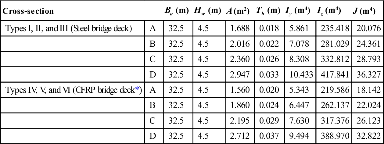
*Moment inertia for bending (Iy and Iz) and torsion (J) of the cross sections of the girder with a CFRP bridge deck listed in Table 8.3 were obtained using an equivalent pure steel cross-section. Bu, width of girder; Hw, depth of girder; A, area of girder; Th, thickness of bridge deck; Iy and Iz, moment inertia for bending along y and z directions, respectively; and J, moment inertia for torsion.
There are several commercially produced CFRP stay cables (namely, Leadline, manufactured and distributed by Mitsubishi Chemical Company, and CFCC, developed by Tokyo Rope Mfg. Co. Ltd) with an elastic modulus from 130 to 160 GPa (Zhang et al., 2001; Grace et al., 2002; Jackson et al., 2005). For the CFRP stay cables (including the CFRP part of the hybrid stay cables) in this case study a value of 137 GPa was used for the elastic modulus based on a widely-used type of CFCC-brand CFRP stay cables (Xiong et al., 2011, 2012). For the CFRP bridge deck the elastic modulus was set as 135 GPa (Xiong et al., 2011). Steel with Chinese grades of Q345qD and Q420qD (with yield stress = 345 and 420 MPa; allowable stress = 190 and 200 MPa for normal static load, and 280 and 345 MPa for wind load, respectively) were used for the girder but the latter could only be used locally. C55 and C60 types of concrete (with allowable compression stress = 17.75 and 19.25 MPa, respectively) were used for the pylons. The cable-stayed bridges were designed to carry eight traffic lanes in two directions and the secondary dead load was assumed to be 70 kN/m. The design wind velocity Vd for the bridge was 74.9 m/s using the assumed bridge site information.
The finite element (FE) models of the six bridges were created using ANSYS program, see Fig. 8.17d. The bridge decks, girders, diaphragms, and pylons were all modeled using beam elements with certain cross-section inputs (in total 4674 elements were used) which have three translational degrees of freedom (DOFs) and three rotational DOFs for each node (4659 nodes were used in total). The stay cables were modeled using spar (truss) elements with ten elements for each stay cable and three translational DOFs for each node (Freire et al., 2006). The nodes of girders located at the diaphragms were meshed using structural mass elements with an initial input of torsion moments of inertia (the rotary inertia can be assigned in each coordinate direction). By doing this, the torsion moments of inertia provided by the diaphragms that increase the torsion stiffness of the bridge girder can be independently added to the girders of the beam elements. For each model the girder and pylons at the girder–pylon connections are free to move longitudinally.
8.5.2 Mechanical behavior and a comparative study
To compare the use of different combinations of CFRP and steel materials, the results of all six bridges for one specific parameter are discussed. The Type I bridge using only traditional steel and concrete materials is treated as a reference model in the following comparative study.
The reasonable dead load conditions for the six bridges (Types I–VI) as shown in Fig. 8.19a and 8.19b were obtained using the proposed design strategies, analytical procedures, and finite element models. As expected, the bending moments of girders (half span) (Fig. 8.19a) and the stresses of pylons (Fig. 8.19b) in the reasonable dead load conditions are within an appropriate range as predicted on the basis of practical engineering experience (Gimsing, 1997; Nagai et al., 2004). The bending moments of girders with a CFRP bridge deck i.e. Types IV, V, and VI, are slightly lower than those with a steel bridge deck i.e. Types I, II, and III. It is noted that the peaks of moments at the locations of piers shown in Fig. 8.19a can be greatly reduced in the construction process if necessary. Based on the results, it can be concluded that following the introduced analytical procedure the reasonable dead load conditions of the cable-stayed bridges with CFRP components i.e. Types II to VI bridges can be designed to be quite similar to those of the reference Type I bridge.

The reasonable stay cable forces are shown in Plate VIII (in the color section between pages 172 and 173) (half span). As expected, due to the light self-weight of CFRP bridge decks, the reasonable stay cable forces of Types IV, V, and VI bridges are much smaller than those of Types I, II, and III. Therefore, using CFRP bridge decks can significantly decrease the amount of material used for stay cables, further reducing the self-weight of bridges and reducing the necessary foundations. However, only negligible differences in the reasonable stay cable forces are found if the stay cable materials are changed from steel to CFRP materials (Types I vs III and IV vs VI).
Figure 8.20a–8.20f show the structural performance of several components of interest under a moving HS20 truck (AASHTO, 2004) vs the vehicle location of the rear axle along the bridge span. It can be seen from Fig. 8.20a that the vertical displacements at the mid span of the bridges with a CFRP bridge deck i.e. Types IV, V, and VI, are clearly larger than those of the bridges with a steel bridge deck i.e. Types I, II, and III, which indicates a decrease in global stiffness by using CFRP bridge decks. This decrease is mainly due to the lower elastic modulus of CFRP materials and lower stay cable forces and stiffness. Furthermore, among all the cases using CFRP bridge decks, the vertical displacement at the mid span of the Type VI bridge with CFRP stay cables is larger than that of the Type V bridge with hybrid stay cables. Both are larger than that of the Type IV bridge with steel stay cables. This indicates that both CFRP bridge decks and CFRP stay cables tend to reduce the global stiffness of bridges, although the decrease is insignificant and acceptable in engineering practice. This conclusion can also be supported by the results of horizontal displacements at the top of the pylons and bending moments at their bottom, as shown in Fig. 8.20b and 8.20c respectively, since both have a direct correlation with the vertical displacements at the mid span.
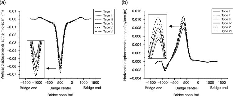
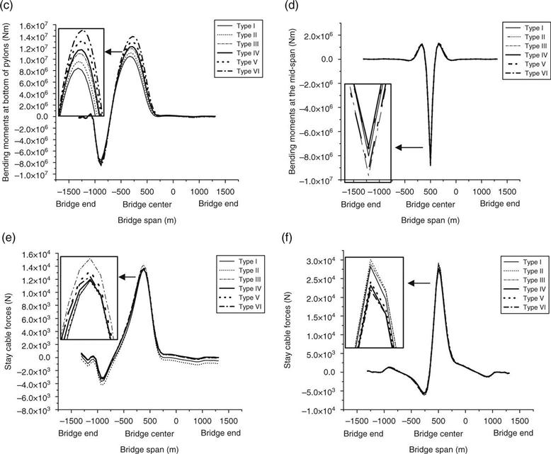
Figure 8.20d shows that the bending moments at mid span are very close to each other, which means that the low global stiffness of the bridge due to CFRP components has only marginal effect on the bending moments of the girders. Figure 8.20e and 8.20f show an insignificant effect of CFRP components on the stay cable force variations under the moving truck loading. Cable No. 1 is the longest cable in the side span and No. 76 is the longest one in the center span.
The cases using heavier or more trucks show similar results. It should be noted that all these results are only for bridges of 1400 m span length. With the extension of bridge span lengths, the equivalent elasticity modulus of steel stay cables will be greatly reduced in contrast to that of the lighter CFRP stay cables. Therefore it can be predicted that the global stiffness of bridges with hybrid and CFRP stay cables may eventually be higher than those with steel stay cables. A study in this regard is ongoing by the authors.
The natural frequencies and mode shapes of the six bridges are presented in Table 8.6 and several significant conclusions can be drawn. The reason for including 16 modes for each case is to include a torsion mode shape. By generally comparing the results of Types I, II, and III bridges with Types IV, V, and VI it is clear that CFRP bridge decks can result in a significant increase in natural frequency.
Table 8.6
Natural frequencies and mode shapes of each bridge type
| Order of mode | Type I | Type II | Type III | Type IV | Type V | Type VI | ||||||
| Freq. (Hz) | Mode shape | Freq. (Hz) | Mode shape | Freq. (Hz) | Mode shape | Freq. (Hz) | Mode shape | Freq. (Hz) | Mode shape | Freq. (Hz) | Mode shape | |
| 1 | 0.0523 | 1st sym. L (girder) | 0.0533 | 1st sym. L (girder) | 0.0537 | 1st sym. L (girder) | 0.0595 | 1st sym. L (girder) | 0.0608 | 1st sym. L (girder) | 0.0615 | 1st sym. L (girder) |
| 2 | 0.0638 | LM (girder) and LB (pylon) | 0.0650 | LM (girder) and LB (pylon) | 0.0655 | LM (girder) and LB (pylon) | 0.0704 | LM (girder) and LB (pylon) | 0.0717 | LM (girder) and LB (pylon) | 0.0722 | LM (girder) and LB (pylon) |
| 3 | 0.1239 | 1st anti. L (girder) | 0.1250 | 1st anti. L (girder) | 0.1255 | 1st anti. L (girder) | 0.1445 | 1st anti. L (girder) | 0.1461 | 1st anti. L (girder) | 0.1468 | 1st anti. L (girder) |
| 4 | 0.1722 | sym. L (pylon) | 0.1735 | sym. L (pylon) | 0.1742 | sym. L (pylon) | 0.1735 | sym. L (pylon) | 0.1746 | sym. L (pylon) | 0.1751 | sym. L (pylon) |
| 5 | 0.1723 | anti. L (pylon) | 0.1737 | anti. L (pylon) | 0.1743 | anti. L (pylon) | 0.1737 | anti. L (pylon) | 0.1747 | anti. L (pylon) | 0.1752 | anti. L (pylon) |
| 6 | 0.1986 | 1st sym. V (girder) | 0.1852 | 1st sym. V (girder) | 0.1771 | 1st sym. V (girder) | 0.2026 | 1st sym. V (girder) | 0.1892 | 1st sym. V (girder) | 0.1812 | 1st sym. V (girder) |
| 7 | 0.2312 | 2nd sym. L (girder) | 0.2266 | 1st anti. V (girder) | 0.2160 | 1st anti. V (girder) | 0.2582 | 1st anti. V (girder) | 0.2393 | 1st anti. V (girder) | 0.2282 | 1st anti. V (girder) |
| 8 | 0.2447 | 1st anti. V (girder) | 0.2353 | 2nd sym. L (girder) | 0.2373 | 2nd sym. L (girder) | 0.2698 | 2nd sym. L (girder) | 0.2750 | 2nd sym. L (girder) | 0.2776 | 2nd sym. L (girder) |
| 9 | 0.3098 | 2nd sym. V (girder) | 0.2962 | 2nd sym. V (girder) | 0.2868 | 2nd sym. V (girder) | 0.3230 | 2nd sym. V (girder) | 0.3102 | 2nd sym. V (girder) | 0.3012 | 2nd sym. V (girder) |
| 10 | 0.3568 | 2nd anti. V (girder) | 0.3457 | 2nd anti. V (girder) | 0.3373 | 2nd anti. V (girder) | 0.3749 | 2nd anti. V (girder) | 0.3665 | 2nd anti. V (girder) | 0.3596 | 2nd anti. V (girder) |
| 11 | 0.3852 | 2nd anti. L (girder) | 0.3824 | 3rd sym. V (girder) | 0.3697 | 3rd sym. V (girder) | 0.4255 | 3rd sym. V (girder) | 0.4025 | 3rd sym. V (girder) | 0.3889 | 3rd sym. V (girder) |
| 12 | 0.4041 | 3rd sym. V (girder) | 0.3906 | 2nd anti. L (girder) | 0.3933 | 2nd anti. L (girder) | 0.4485 | 2nd anti. L (girder) | 0.4560 | 2nd anti. L (girder) | 0.4446 | 3rd anti. V (girder) |
| 13 | 0.4624 | 3rd anti. V (girder) | 0.4372 | 3rd anti. V (girder) | 0.4228 | 3rd anti. V (girder) | 0.4672 | sym. T (girder) and L (pylon) | 0.4595 | 3rd anti. V (girder) | 0.4596 | 2nd anti. L (girder) |
| 14 | 0.4626 | sym. T (girder) and L (pylon) | 0.4694 | sym. T (girder) and L (pylon) | 0.4530 | 4th sym. V (girder) | 0.4682 | anti. T (girder) and L (pylon) | 0.4727 | sym. T (girder) and L (pylon) | 0.4753 | sym. T (girder) and L (pylon) |
| 15 | 0.4635 | anti. T (girder) and L (pylon) | 0.4703 | anti. T (girder) and L (pylon) | 0.4727 | sym. T (girder) and L (pylon) | 0.4861 | 3rd anti. V (girder) | 0.4733 | anti. T (girder) and L (pylon) | 0.4759 | anti. T (girder) and L (pylon) |
| 16 | 0.5029 | 4th sym. V (girder) | 0.4713 | 4th sym. V (girder) | 0.4737 | anti. T (girder) and L (pylon) | 0.5109 | sym. L (pylon) | 0.5017 | 4th sym. V (girder) | 0.4830 | 4th sym. V (girder) |

Notes: L, lateral bending; V, vertical bending; T, torsion; LM, longitudinal moving; LB, longitudinal bending; sym., symmetric; anti., antisymmetric.
The natural frequencies of the vertical bending modes of the bridges with hybrid and CFRP stay cables i.e. Types II and III are slightly lower than those of the bridge with steel stay cables i.e. Type I. This is mainly due to the lower equivalent elasticity modulus of hybrid and CFRP stay cables, which can decrease the supporting stiffness to the girder by the stay cables. The opposite conclusion could be reached if considering the various effects of stay cable materials on bridge stiffness when the bridge span is extended beyond 1400 m.
On the other hand, the natural frequencies of the lateral bending modes of Types II and III bridges are higher than those of Type I. Since the contribution of stay cables to the lateral stiffness of the girders is small, the light weight of CFRP materials may be the main reason for the higher frequencies. In addition, the natural frequencies of torsion modes in Types II and III bridges are higher than those in Type I, due to the light weight of CFRP materials. The same conclusions can also be obtained for the cases of CFRP bridge decks shown at the bottom part of Table 8.6 (Types IV, V, and VI).
Using the natural frequencies of torsion and vertical bending modes in Table 8.6, the critical wind speed due to a flutter phenomenon (Vcr) for each bridge type was calculated and shown in Table 8.7. It can clearly be seen that all the Vcr are higher than the design wind velocity Vd, i.e., 74.9 m/s. By comparing these values, high natural frequencies of torsion modes can increase the Vcr value; however, a decrease of Vcr can also be observed when using light CFRP bridge decks, due to the lower μ values. Referring to Vcr = 51 m/s (bridge over the Dala, Switzerland) and Vcr = 111 m/s (bridge at Diepoldsau, Switzerland) (Walther et al., 1999) all the Vcr of the six bridges are acceptable in most field applications, although the bridges with a CFRP bridge deck could have slightly lower Vcr than those using steel bridge decks. When necessary, the critical wind velocity of bridges with a CFRP deck can be enhanced with many other countermeasures, such as streamlining the deck shape, though it is beyond the scope of the present study.
Table 8.7
Critical wind speed due to flutter phenomenon
| ηs | ηα | fT | fB | ε | r (m) | m (kg/m) | b (m) | μ | ωB | Vcr (m/s) | |
| Type I | 0.9 | 0.7 | 0.4626 | 0.1986 | 2.3293 | 11.8096 | 26588 | 16.25 | 24.6539 | 1.2478 | 96.7 |
| Type II | 0.9 | 0.7 | 0.4694 | 0.1852 | 2.5346 | 11.8096 | 26588 | 16.25 | 24.6539 | 1.1636 | 99.0 |
| Type III | 0.9 | 0.7 | 0.4727 | 0.1771 | 2.6691 | 11.8096 | 26588 | 16.25 | 24.6539 | 1.1128 | 100.1 |
| Type IV | 0.9 | 0.7 | 0.4672 | 0.2026 | 2.3060 | 11.8651 | 20511 | 16.25 | 19.0190 | 1.2730 | 87.5 |
| Type V | 0.9 | 0.7 | 0.4727 | 0.1892 | 2.4984 | 11.8651 | 20511 | 16.25 | 19.0190 | 1.1888 | 89.1 |
| Type VI | 0.9 | 0.7 | 0.4753 | 0.1812 | 2.6231 | 11.8651 | 20511 | 16.25 | 19.0190 | 1.1385 | 90.0 |

ηs = Vc(0°)/Vco, correction coefficient of cross-section shape; ηα = Vc(α)/Vc(0°), correction coefficient of an angle of incidence σ; Vco = theoretical critical wind speed of flat plate due to flutter phenomenon fT and fB = natural frequencies of torsion mode and vertical bending mode, respectively; ωT and ωB = natural circular frequencies of torsion mode and vertical bending mode, respectively; ε = ωT/ωB = fT/fB, ratio of natural frequency of torsion mode to that of vertical bending mode; r = radius of gyration; m = mass per unit length of girder; b = half width of deck; ρ = density of air (1.3 kg/m3); μ = πρb2; and Vcr = critical wind speed due to flutter phenomenon.
Again, the safety factor of the hybrid stay cables remained as 2.5, consistent with other types of bridges to provide a convenient comparison. Actually, as discussed earlier, increasing the safety factor could be a good way to enhance the mechanical performance of the hybrid stay cables. Therefore, according to this comparative study, cable-stayed bridges with hybrid stay cables (Types II and IV) could potentially have better mechanical performances by increasing the safety factor under different design criteria.
8.5.3 Economic aspects and a comparative study
In addition to the mechanical behavior, economic aspects (material and construction cost) also need to be studied to examine the feasibility of a new cable-stayed bridge type using CFRP components. Using the six selected cable-stayed bridges, the cost for the stay cables and bridge girder and deck can be directly calculated from the previous design. However, the cost of the substructure (including pylons) needs to be estimated following the discussions below.
Analytical model for cost study of substructures
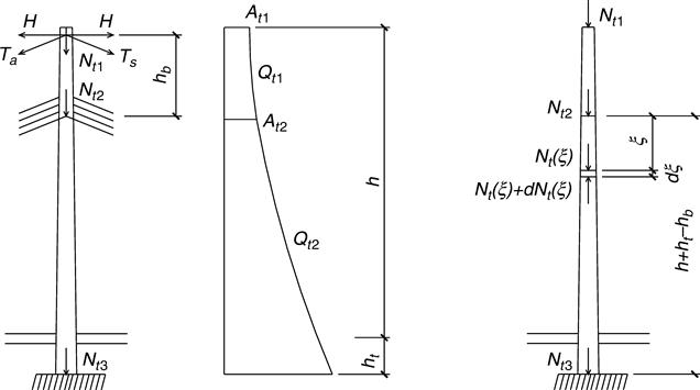
In this section, the pylon component is simplified as a column under an axial compression load, as shown in Fig. 8.21. Some assumptions need to be followed:
(a) cross-sectional area of the pylon in the anchorage zone is varied linearly, based on the varying compression loads (At1 = cross-sectional area at the top pylon; and At2 = cross-sectional area at the bottom of the anchorage zone in the pylon);
(b) a no-anchorage zone is seen as a column under a constant axial compression load.
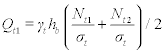
I Material amount (weight) of anchorage zone in the pylon Qt1
[8.22]
where:
γt = density of pylon materials; and
hb = height of anchorage zone in pylon.
The axial compression loads at the top pylon, Nt1, can be calculated as:
[8.23]
where:
H = horizontal component of the first stay cable forces, assuming the one on the left side equal to the right side (in Fig. 8.21a); and
α and β = incline angle of stay cables on the left and right side of the pylon, respectively.
Then the cross-sectional area at the top pylon can be obtained as:
[8.24]
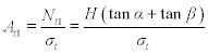 [8.24]
where:
σt = allowable compressive stress of the pylon materials.
Other parameters can be found in Fig. 8.21a.
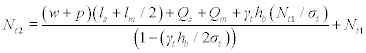
The axial compression loads at the bottom of the anchorage zone in the pylon, Nt2, can also be calculated using the equilibrium equations shown below:
[8.25]
[8.26]
 [8.26]
where:
w and p = uniform gravity loads and distributed live loads per unit length of the girder, respectively;
ls and lm = side span and main span length of the cable-stay bridge, respectively;
Qs and Qm = self-weight of stay cables in the side span and main span of the cable-stay bridge, respectively (corresponding to one pylon); and
Qt1 = self-weight of the pylon in the anchorage zone.
Then, Equations [8.25] and [8.26] give:
[8.27]
 [8.27]
Substituting Equations [8.23] and [8.27] into Equation [8.26], the material amount of an anchorage zone in the pylon, Qt1, can be finally estimated.
II Material amount (weight) of no-anchorage zone in the pylon Qt2
Figure 8.21b apparently gives:
[8.28]
where:
Nt(ξ) = axial compression loads in the pylon; and
ξ = section distance from where Nt2 applies.
Therefore,
[8.29]
The differential equation of Nt(ξ) is then calculated as:
[8.30]
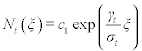 [8.30]
where c1 = any arbitrary constant.
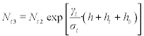
Substituting the boundary conditions that ξ = 0 and Nt(0) = Nt2 into Equation [8.30], the variable axial force Nt(ξ) can be solved:
[8.31]
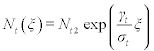 [8.31]
Then the material amount of a none-anchorage zone in the pylon, Qt2, can be easily calculated:
[8.32]
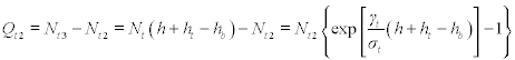 [8.32]
where Nt3 = axial compression loads at the bottom of the pylon.
III. Cost for one pylon
Based on the values of Qt1 and Qt2, the cost for one pylon can be expressed as:
[8.33]
where:
Qt = material amount of one pylon; and
μt = cost (price) per unit weight.
IV. Cost for foundation structures
Based on Equation [8.31] the reaction force at the location of one pylon can be calculated as:
[8.34]
 [8.34]
All the reaction force of the half bridge structure, W, is:
[8.35]
The reaction force taken by the side and abutment piers in the half span, Nb, is:
[8.36]
Then, the material amount of foundation structures at the location of pylon and piers of the first half span bridge can be written as:
[8.37]
[8.38]
where:
Qj and Qb = material amount (weight) of the foundation structures at the location of pylon and piers of the first half span bridge, respectively; and
kj and kb = weight coefficients for the pylon and piers respectively, both of which are equal to 4.0 based on the Chinese code for budget estimate of bridge engineering in the present study, or are determined by the designers’ experiences (JTG B06–2007, 2007).
Based on the values of Qj and Qb, the cost for the foundation structures in the half span can be obtained as:
[8.39]
where μj and μb = cost (price) per unit weight for the pylon and piers, respectively.
V. Cost for substructures
Finally, the substructure cost (including pylons) for the whole bridge structure can be calculated using the expression below:
[8.40]
Discussion of economic aspects of each bridge type
For the purposes of comparison, the current cost of each main component in the six selected bridge cases is assumed in Table 8.8 (JTG B06–2007, 2007).
Table 8.8
Current cost for each main component
| Components | Cost | Components | Cost |
| Steel stay cables | $3.0/kg | Steel girder | $3.3/kg |
| CFRP stay cable | $80.0/kg | Concrete pylon | $0.3/kg |
| Steel bridge deck | $3.3/kg | Foundation | $0.2/kg |
| CFRP bridge deck | $85.0/kg | Piers | $0.2/kg |

Based on Equations [8.22]–[8.40], costs listed in Table 8.8, and design parameters already obtained from bridge models, the overall costs required for the six cable-stayed bridges using CFRP components can be directly calculated and are shown in Table 8.9. The area ratio of the hybrid stay cables (Type II and Type V) is 0.6 based on the results in Section 8.4.3.
Table 8.9
Costs for the six types of cable-stayed bridges
| Components/bridge types | Type 1 | Type II | Type III | Type IV | Type V | Type VI | |
| Superstructure (Million $) | Steel stay cables | 75.20 | 26.39 | – | 54.89 | 19.79 | – |
| CFRP stay cables | – | 145.21 | 220.22 | – | 108.9 | 162.97 | |
| Total for cables (percentage of total) | 75.19 (11.5%) | 171.60 (24.1%) | 220.23 (31.6%) | 54.89 (6.6%) | 128.71 (14.6%) | 162.97 (18.8%) | |
| Girder and deck (percentage of total) | 234.58 (35.9%) | 234.58 (33.0%) | 234.58 (33.6%) | 524.84 (63.2%) | 524.84 (59.5%) | 524.84 (60.5%) | |
| Subtotal (percentage of total) | 309.77 (47.4%) | 406.19 (57.1%) | 454.80 (65.2%) | 579.73 (69.8%) | 653.54 (74.1%) | 687.81 (79.3%) | |
| Pylon (Million $) (percentage of total) | 74.41 (11.4%) | 66.16 (9.3%) | 52.60 (7.5%) | 54.32 (6.5%) | 49.62 (5.6%) | 38.92 (4.5%) | |
| Pier (Million $) (percentage of total) | 268.84 (41.2%) | 239.05 (33.6%) | 190.02 (27.2%) | 196.26 (23.6%) | 179.29 (20.3%) | 140.61 (16.2%) | |
| Total cost (Million $) | 653.02 | 711.40 | 697.42 | 830.30 | 882.45 | 867.34 | |
| Total cost per span length (Million $/m) | 0.3207 | 0.3494 | 0.3425 | 0.4078 | 0.4334 | 0.426 | |
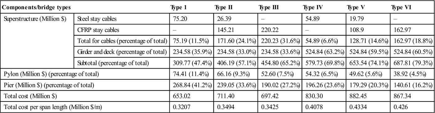
According to Table 8.9, the cost of both CFRP stay cables and bridge deck is still higher than that of steel design even though their light self-weight can significantly reduce the cost of the substructures. The designs using hybrid stay cables (Types II and V) are a little more expensive than others using pure steel or CFRP materials as stay cables. It can be concluded that the cable-stayed bridges using CFRP materials do not reflect any initial cost benefit from the current price of CFRP materials. However, CFRP materials may have life-cycle cost benefits that are not discussed here.
Also when it comes to costs, the factor of varying price for each material needs to be further considered. The current price ratio of CFRP to steel materials is roughly determined as 27/1. The CFRP material price has been significantly reduced in the last decade and will be further reduced in the near future, which will lower the price ratio used in Table 8.9 and lead to different conclusions.
Figure 8.22 shows the varying cost of the six cable-stayed bridges or their components based on a cost ratio variation of CFRP to steel materials from 27/1 to 2/1. All the costs for components or the entire bridge using CFRP materials could be reduced significantly with a decrease in the price ratio from 27/1 to 2/1, especially for the cases with both CFRP stay cables and CFRP bridge decks (Types III and VI). The cost percentage of each component is also seen in Fig. 8.22b and 8.22d. Both reductions on CFRP stay cables and bridge deck can result in an increasing percentage of costs for substructure (piers and pylons), which is shown in Fig. 8.22e.
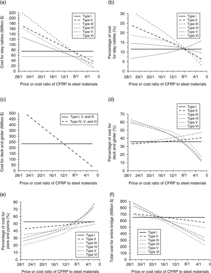
In summary, Fig. 8.22 shows that using CFRP materials for the components or entire bridge could be more cost-effective than the traditional design when the price ratio is over a certain value. For example, in Fig. 8.22a for stay cable cost, when the price ratio is less than 8/1 the stay cables using CFRP materials (Types II, III, V, and VI) are more economical than steel ones; while in Fig. 8.22f looking at the total cost, this dividing ratio value is 16/1 for those using CFRP components (Types II–VI). Due to the large amount of material in the bridge deck, the cases using CFRP bridge deck (Types IV–VI) could show greater economic benefit from the reduced price ratio. It is logical to predict that the advantages of using CFRP components will be further enhanced with the rapid decrease in the cost of CFRP materials. In the near future, the proposed cable-stayed bridges using CFRP stay cables and/or CFRP bridge deck could be an excellent alternative to the traditional steel cable-stayed bridges, not only from a mechanical viewpoint but also from an economical viewpoint.
8.6 Conclusions and future trends
Based on the numerical study, cable-stayed bridges with CFRP components (CFRP bridge deck, CFRP stay cables, and hybrid stay cables) can be an excellent alternative to traditional steel cable-stayed bridges, especially for bridges with super-long spans. Although in the present study only the cable-stayed bridges with a main span length of 1400 m were studied, it can still be predicted that the advantages of using CFRP components will be further enhanced with the continuous extension of bridge span lengths and decreasing cost of CFRP materials. For future work, a study of the span extension/ limitation and construction design for the proposed cable-stayed bridges with CFRP components are also needed.
8.7 Acknowledgments
This work was partially supported by the grant from National Natural Science Foundation of China (NSFC) (Project No. 51229801), Specialized Research Fund for the Doctoral Program of Higher Education (Project No. 20120092120058), and Natural Science Foundation of Jiangsu Province of China (Project No. BK2012343). The contents presented reflect only the views of the writers who are responsible for the facts and the accuracy of the data presented herein.