Equations
This appendix describes some important formulas and matrices referred to in the text.
B.1 3D Vectors
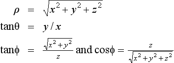
B.1.1 Spherical Coordinates
Given a point specified in Cartesian coordinates (x, y, z)T, the spherical coordinates (ρ, θ, φ) consisting of a length and two angles are
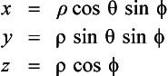
Given length ρ, azimuth angle φ, and elevation angle θ (assuming y is up) the Cartesian coordinates of the corresponding unit vector are
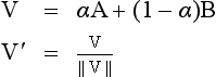
B.1.2 Linear Interpolation of 3D Vectors
Each vector component is interpolated separately, and then the resulting interpolated vector is renormalized. Renormalization is required if the interpolated vectors need to have unit length. Linearly interpolating a vector V using a single parameter α along a line with vectors A and B at the endpoints:
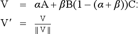
Linearly interpolating a vector V using two barycentric parameters α and β over a triangle with vectors A, B, C at the vertices:
Note: When using linear vector interpolation care must be taken to handle or report the case where one or more vector components interpolate to zero or a number so small that an excessive amount of accuracy is lost in the representation. In cases where linear interpolation is inadequate, spherical interpolation (SLERP) using quaternions may be a preferable method.
B.1.3 Barycentric Coordinates
Given a triangle with vertices A, B, C, the barycentric coordinates of the point P inside triangle ABC are α, β, γ, with P = αA + βB + γC and α + β + γ = 1. Let area (XYZ) be the area of the triangle with vertices X, Y, Z. Then
and the barycentric coordinates are the ratios of the areas of the subtriangles formed by the interior point P to the entire triangle ABC:
B.2 Projection Matrices
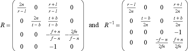
The call glOrtho(l, r, b, t, u, f) generates R, where
R is defined as long as l ≠ r, t ≠ b, and n ≠ f.
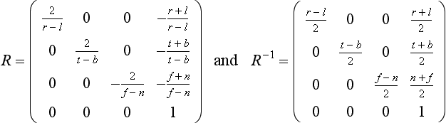
B.2.2 Perspective Projection
The call glFrustum(l, r, b, t, n, f) generates R, where
R is defined as long as l ≠ r, t ≠ b, and n ≠ f.
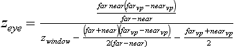
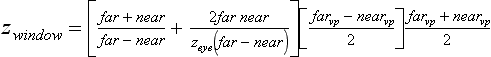
B.2.3 Perspective z-Coordinate Transformations
The z value in eye coordinates, zeye, can be computed from the window coordinate z value, zwindow, using the near and far plane values, near and far, from the glFrustum command and the viewport near and far values, farvp and nearvp, from the glDepthRange command using the equation
The z-window coordinate is computed from the eye coordinate z using the equation
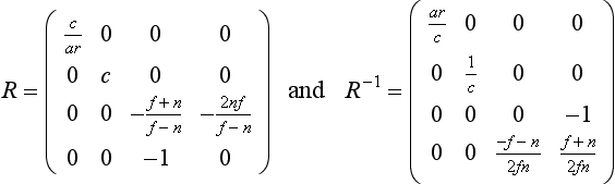
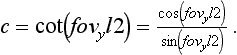 . R is defined as long as ar ≠ 0, sin(fovy) ≠ 0, and n ≠ f.
B.3 Viewing Transforms
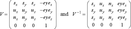
The call gluLookat(eyex, eyey, eyez, centerx, centery, centerz, upx, upy, upz) generates V, where
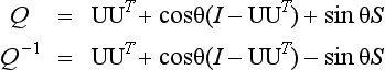
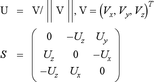
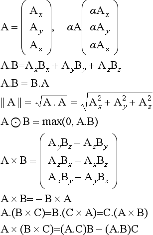
B.5 Parallel and Perpendicular Vectors
Given two vectors A, B, the portion of A parallel to B is
and the proportion of A perpendicular to B is A⊥B = A − A![]() B.
B.
B.6 Reflection Vector
Given a surface point p, a unit vector, N, normal to that surface, and a vector, U, incident to the surface at p, the reflection vector, R, exiting from p is
If U′ is exiting from the surface, U′ = − U and
B.7 Lighting Equations
In single-color lighting mode, the primary and secondary colors at surface point Ps are computed from n light sources as
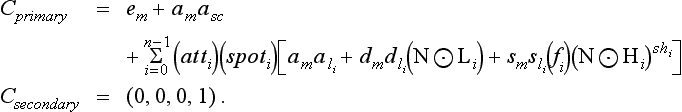
In separate specular color mode, the primary and secondary colors are computed from n light sources as
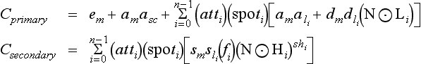
where
em, am, dm, and sm are the material emissive, ambient, diffuse, and specular reflectances
asc is the scene ambient intensity
![]() , and
, and ![]() are the ambient, diffuse, and specular intensities for light source i
are the ambient, diffuse, and specular intensities for light source i
where,
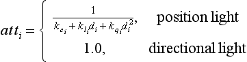
di is the distance between the surface point and light source i
![]() is the constant attenuation for light source i
is the constant attenuation for light source i
spoti is the spotlight attenuation for light source i
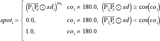
sdi is the spotlight direction unit vector for light source i
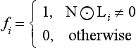
N is the surface normal unit vector Li is the unit vector from the surface point to light source i, ![]()
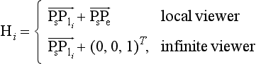
Hi is the half-angle vector between the vectors from the surface point to the eye position (Pe), and the surface point and and light source i
B.8 Function Approximations
The Taylor series expansion of a function f(x) about the point a is
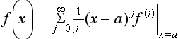
where f(j) denotes the jth derivative of f(x). The Maclaurin series expansion is the special case of the Taylor series expansion about the point a = 0.
B.8.2 Newton-Raphson Method
The Newton-Raphson method for obtaining a root of the function f(x) uses an initial estimate x0 and the recurrence
The approximation for the reciprocal of a number a is the root of the equation f(x) = 1/x−a. Substituting f(x) in Equation B.1 gives
and the reciprocal square root of a number a is the root of the equation f(x) = 1/x2 − a. Substituting f(x) in Equation B.1 gives
B.8.3 Hypotenuse
A rough approximation of the 2D hypotenuse or length function ![]() suitable for level-of-detail computations (Wu, 1988), is
suitable for level-of-detail computations (Wu, 1988), is