CAD and Modeling Techniques
In previous chapters, many of the underlying principles for faithful rendering of models have been described. In this chapter, we extend those techniques with additional algorithms that are particularly useful or necessary for interactive modeling applications such as those used for computer-aided design (CAD). The geometric models use complex representations such as NURBS surfaces and geometric solids that are typically converted to simpler representations for display. Representations for even relatively simple real-world objects can involve millions of primitives. Displaying and manipulating large models both efficiently and effectively is a considerable challenge. Besides the display of the model, CAD applications must also supply other information such as labels and annotations that can also challenge efficient display. CAD applications often include a variety of analysis and other tools, but we are primarily concerned with the display and interactive manipulation parts of the application.
16.1 Picking and Highlighting
Interactive selection of objects, including feedback, is an important part of modeling applications. OpenGL provides several mechanisms that can be used to perform object selection and highlighting tasks.
16.1.1 OpenGL Selection
OpenGL supports an object selection mechanism in which the object geometry is transformed and compared against a selection subregion (pick region) of the viewport. The mechanism uses the transformation pipeline to compare object vertices against the view volume. To reduce the view volume to a screen-space subregion (in window coordinates) of the viewport, the projected coordinates of the object are transformed by a scale and translation transform and combined to produce the matrix
where ox, oy, px, and py are the x and y origin and width and height of the viewport, and qx, qy, dx, and dy are the origin and width and height of the pick region.
Objects are identified by assigning them integer names using glLoadName. Each object is sent to the OpenGL pipeline and tested against the pick region. If the test succeeds, a hit record is created to identify the object. The hit record is written to the selection buffer whenever a change is made to the current object name. An application can determine which objects intersected the pick region by scanning the selection buffer and examining the names present in the buffer.
The OpenGL selection method determines that an object has been hit if it intersects the view volume. Bitmap and pixel image primitives generate a hit record only if a raster positioning command is sent to the pipeline and the transformed position lies within the viewing volume. To generate hit records for an arbitrary point within a pixel image or bitmap, a bounding rectangle should be sent rather than the image. This causes the selection test to use the interior of the rectangle. Similarly, wide lines and points are selected only if the equivalent infinitely thin line or infinitely small point is selected. To facilitate selection testing of wide lines and points, proxy geometry representing the true footprint of the primitive is used instead.
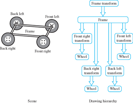
Many applications use instancing of geometric data to reduce their memory footprint. Instancing allows an application to create a single representation of the geometric data for each type of object used in the scene. If the application is modeling a car for example, the four wheels of the car may be represented as instances of a single geometric description of a wheel, combined with a modeling transformation to place each wheel in the correct location in the scene. Instancing introduces extra complexity into the picking operation. If a single name is associated with the wheel geometry, the application cannot determine which of the four instances of the wheel has been picked. OpenGL solves this problem by maintaining a stack of object names. This allows an application, which represents models hierarchically, to associate a name at each stage of its hierarchy. As the car is being drawn, new names are pushed onto the stack as the hierarchy is descended and old names are popped as the hierarchy is ascended. When a hit record is created, it contains all names currently in the name stack. The application determines which instance of an object is selected by looking at the content of the name stack and comparing it to the names stored in the hierarchical representation of the model.
Using the car model example, the application associates an object name with the wheel representation and another object name with each of the transformations used to position the wheel in the car model. The application determines that a wheel is selected if the selection buffer contains the object name for the wheel, and it determines which instance of the wheel by examining the object name of the transformation. Figure 16.1 shows an illustration of a car frame with four wheels drawn as instances of the same wheel model. The figure shows a partial graph of the model hierarchy, with the car frame positioned in the scene and the four wheel instances positioned relative to the frame.
When the OpenGL pipeline is in selection mode, the primitives sent to the pipeline do not generate fragments to the framebuffer. Since only the result of vertex coordinate transformations is of interest, there is no need to send texture coordinates, normals, or vertex colors, or to enable lighting.
16.1.2 Object Tagging in the Color Buffer
An alternative method for locating objects is to write integer object names as color values into the framebuffer and read back the framebuffer data within the pick region to reconstruct the object names. For this to work correctly, the application relies on being able to write and read back the same color value. Texturing, blending, dithering, lighting, and smooth shading should be disabled so that fragment color values are not altered during rasterization or fragment processing. The unsigned integer forms of the color commands (such as glColor3ub) are used to pass in the object names. The unsigned forms are defined to convert the values in such a way as to preserve the b most significant bits of the color value, where b is the number of bits in the color buffer. To limit selection to visible surfaces, depth testing should be enabled. The back color buffer can be used for the drawing operations to keep the drawing operations invisible to the user.
A typical RGB color buffer, storing 8-bit components, can represent 24-bit object names. To emulate the functionality provided by the name stack in the OpenGL selection mechanism, the application can partition the name space represented by a color value to hold instancing information. For example, a four level hierarchy can subdivide a 24-bit color as 4, 4, 6, and 10 bits. Using 10 bits for the lowest level of the hierarchy creates a larger name space for individual objects.
One disadvantage of using the color buffer is that it can only hold a single identifier at each pixel. If depth buffering is used, the pixel will hold the object name corresponding to a visible surface. If depth buffering is not used, a pixel holds the name of the last surface drawn. The OpenGL selection mechanism can return a hit record for all objects that intersect a given region. The application is then free to choose one of the intersecting objects using a separate policy. A closest-to-viewer policy is simple using either OpenGL selection or color buffer tags. Other policies may need the complete intersection list, however. If the number of potential objects is small, the complete list can be generated by allocating nonoverlapping names from the name space. The objects are drawn with bitwise OR color buffer logic operations to produce a composite name. The application reconstructs the individual objects names from the composite list. This algorithm can be extended to handle a large number of objects by partitioning objects into groups and using multiple passes to determine those groups that need more detailed interrogation.
16.1.3 Proxy Geometry
One method to reduce the amount of work done by the OpenGL pipeline during picking operations (for color buffer tagging or OpenGL selection) is to use a simplified form of the object in the picking computations. For example, individual objects can be replaced by geometry representing their bounding boxes. The precision of the picking operation is traded for increased speed. The accuracy can be restored by adding a second pass in which the objects, selected using their simplified geometry, are reprocessed using their real geometry. The two-pass scheme improves performance if the combined complexity of the proxy objects from the first pass and the real objects processed in the second pass is less than the complexity of the set of objects tested in a single-pass algorithm.
16.1.4 Mapping from Window to Object Coordinates
For some picking algorithms it is useful to map a point in window coordinates (xw, yw, zw)T to object coordinates (x0, y0, z0)T. The object coordinates are computed by transforming the window coordinates by the inverse of the viewport V, projection P, and modelview M transformations:
This procedure isn’t quite correct for perspective projections since the inverse of the perspective divide is not included. Normally, the w value is discarded after the perspective divide, so finding the exact value for wclip may not be simple. For applications using perspective transformations generated with the glFrustum and gluPerspective commands, the resulting wclip is the negative eye-space z coordinate, −ze. This value can be computed from zw using the viewport and projection transform parameters as described in Appendix B.2.3.
In some situations, however, only the window coordinate x and y values are available. A 2D window coordinate point maps to a 3D line in object coordinates. The equation of the line can be determined by generating two object-space points on the line, for example at zw = 0 and zw = 1. If the resulting object-space points are P0 and Q0, the parametric form of the line is
16.1.5 Other Picking Methods
For many applications it may prove advantageous to not use the OpenGL pipeline at all to implement picking. For example, an application may choose to organize its geometric data spatially and use a hierarchy of bounding volumes to efficiently prune portions of the scene without testing each individual object (Rohlf, 1994; Strauss, 1992).
16.1.6 Highlighting
Once the selected object has been identified, an application will typically modify the appearance of the object to indicate that it has been selected. This action is called highlighting. Appearance changes can include the color of the object, the drawing style (wireframe or filled), and the addition of annotations. Usually, the highlight is created by re-rendering the entire scene, using the modified appearance for the selected object.
In applications manipulating complex models, the cost of redrawing the entire scene to indicate a selection may be prohibitive. This is particularly true for applications that implement variations of locate-highlight feedback, where each object is highlighted as the cursor passes over or near it to indicate that this object is the current selection target. An extension of this problem exists for painting applications that need to track the location of a brush over an object and make changes to the appearance of the object based on the current painting parameters (Hanrahan, 1990).
An alternative to redrawing the entire scene is to use overlay windows (Section 7.3.1) to draw highlights on top of the existing scene. One difficulty with this strategy is that it may be impossible to modify only the visible surfaces of the selected object; the depth information is present in the depth buffer associated with the main color buffer and is not shared with the overlay window. For applications in which the visible surface information is not required, overlay windows are an efficient solution. If visible surface information is important, it may be better to modify the color buffer directly. A depth-buffered object can be directly overdrawn by changing the depth test function to GL_LEQUAL and redrawing the object geometry with different attributes (Section 9.2). If the original object was drawn using blending, however, it may be difficult to un-highlight the object without redrawing the entire scene.
16.1.7 XOR Highlighting
Another efficient highlighting technique is to overdraw primitives with an XOR logic operation. An advantage of using XOR is that the highlighting and restoration operations can be done independently of the original object color. The most significant bit of each of the color components can be XORed to produce a large difference between the highlight color and the original color. Drawing a second time restores the original color.
A second advantage of the XOR method is that depth testing can be disabled to allow the occluded surfaces to poke through their occluders, indicating that they have been selected. The highlight can later be removed without needing to redraw the occluders. This also solves the problem of removing a highlight from an object originally drawn with blending. While the algorithm is simple and efficient, the colors that result from XORing the most significant component bits may not be aesthetically pleasing, and the highlight color will vary with the underlying object color.
One should also be careful of interactions between the picking and highlighting methods. For example, a picking mechanism that uses the color or depth buffer cannot be mixed with a highlighting algorithm that relies on the contents of those buffers remaining intact between highlighting operations.
A useful hybrid scheme for combining color buffer tagging with locate-highlight on visible surfaces is to share the depth buffer between the picking and highlighting operations. It uses the front color buffer for highlighting operations and the back color buffer for locate operations. Each time the viewing or modeling transformations change, the scene is redrawn, updating both color buffers. Locate-highlight operations are performed using these same buffers until another modeling or viewing change requires a redraw. This type of algorithm can be very effective for achieving interactive rates for complex models, since very little geometry needs to be rendered between modeling and viewing changes.
16.1.8 Foreground Object Manipulation
The schemes for fast highlighting can be generalized to allow limited manipulation of a selected depth-buffered object (a foreground object) while avoiding full scene redraws as the object is moved. The key idea is that when an object is selected the entire scene is drawn without that object, and copies of the color and depth buffer are created. Each time the foreground object is moved or modified, the color buffer and depth buffer are initialized using the saved copies. The foreground object is drawn normally, depth tested against the saved depth buffer.
This image-based technique is similar to the algorithm described for compositing images with depth in Section 11.5. To be usable, it requires a method to efficiently save and restore the color and depth images for the intermediate form of the scene. If aux buffers or stereo color buffers are available, they can be used to store the color buffer (using glCopyPixels) and the depth buffer can be saved to the host. If off-screen buffers (pbuffers) are available, the depth (and color) buffers can be efficiently copied to and restored from the off-screen buffer. Off-screen buffers are described in more detail in Section 7.4.1. It is particularly important that the contents of the depth buffer be saved and restored accurately. If some of the depth buffer values are truncated or rounded during the transfer, the resulting image will not be the same as that produced by drawing the original scene. This technique works best when the geometric complexity of the scene is very large—so large that the time spent transferring the color and depth buffers is small compared to the amount of time that would be necessary to re-render the scene.
16.2 Culling Techniques
One of the central problems in rendering an image is determining which parts of each object are visible. Depth buffering is the primary method supported within the OpenGL pipeline. However, there are several other methods that can be used to determine, earlier in the pipeline, whether an object is invisible, allowing it to be rejected or culled. If parts of an object can be eliminated earlier in the processing pipeline at a low enough cost, the entire scene can be rendered faster. There are several culling algorithms that establish the visibility of an object using different criteria.
• Back-face culling eliminates the surfaces of a closed object that are facing away from the viewer, since they will be occluded by the front-facing surfaces of the same object.
• View-frustum culling eliminates objects that are outside the viewing frustum. This is typically accomplished by determining the position of an object relative to the planes defined by the six faces of the viewing frustum.
• Portal culling (Luebke, 1995) subdivides indoor scenes into a collection of closed cells, marking the “holes” in each cell formed by doors and windows as portals. Each cell is analyzed to determine the other cells that may be visible through portals, resulting in a network of potentially visible sets (PVS) describing the set of cells that must be drawn when the viewer is located in a particular cell.
• Occlusion culling determines which objects in the scene are occluded by other large objects in the scene.
• Detail culling (like geometric LOD) determines how close an object is to the viewer and adds or removes detail from the object as it approaches or recedes from the viewer.
A substantial amount of research is available on all of these techniques. We will examine the last two techniques in more detail in the following sections.
16.3 Occlusion Culling
Complex models with high depth complexity render many pixels that are ultimately discarded during depth testing. Transforming vertices and rasterizing primitives that are occluded by other polygons reduces the frame rate of the application while adding nothing to the visual quality of the image. Occlusion culling algorithms attempt to identify such nonvisible polygons and discard them before they are sent to the rendering pipeline (Coorg, 1996; Zhang, 1998). Occlusion culling algorithms are a form of visible surface determination algorithm that attempts to resolve visible (or nonvisible surfaces) at larger granularity than pixel-by-pixel testing.
A simple example of an occlusion culling algorithm is backface culling. The surfaces of a closed object that are facing away from the viewer are occluded by the surfaces facing the viewer, so there is no need to draw them. Many occlusion culling algorithms operate in object space (Coorg, 1996; Luebke, 1995) and there is little that can be done with the standard OpenGL pipeline to accelerate such operations. However, Zhang et al. (1997) describe an algorithm that computes a hierarchy of image-space occlusion maps for use in testing whether polygons comprising the scene are visible.
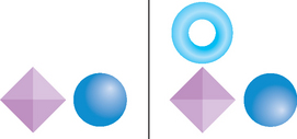
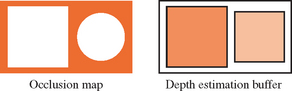
An occlusion map is a 2D array of values; each one measures the opacity of the image plane at that point. An occlusion map (see Figure 16.2) corresponding to a set of geometry is generated by rendering the geometry with the polygon faces colored white. The occlusion map is view dependent. In Zhang’s algorithm the occlusion map is generated from a target set of occluders. The occlusion map is accompanied by a depth estimation buffer that provides a conservative estimate of the maximum depth value of a set of occluders at each pixel. Together, the occlusion map and depth estimation buffer are used to determine whether a candidate object is occluded. A bounding volume for the candidate object is projected onto the same image plane as the occlusion map, and the resulting projection is compared against the occlusion map to determine whether the occluders overlap the portion of the image where the object would be rendered. If the object is determined to be overlapped by the occluders, the depth estimation buffer is tested to determine whether the candidate object is behind the occluder geometry. A pyramidal hierarchy of occlusion maps (similar to a mipmap hierarchy) can be constructed to accelerate the initial overlap tests.
16.3.1 Choosing Occluders
Choosing a good set of occluders can be computationally expensive, as it is approximating the task of determining the visible surfaces. Heuristic methods can be used to choose likely occluders based on an estimation of the size of the occluder and distance from the eye. To maintain interactive rendering it may be useful to assign a fixed polygon budget to the list of occluders. Temporal coherence can be exploited to reduce the number of new occluders that needs to be considered each frame.
16.3.2 Building the Occlusion Map
Once the occluders have been selected they are rendered to the framebuffer with lighting and texturing disabled. The polygons are colored white to produce values near or equal to 1.0 in opaque areas. OpenGL implementations that do not support some form of antialiasing will have pixels values that are either 0.0 or 1.0. A hierarchy of reduced resolution maps is created by copying this map to texture memory and performing bilinear texture filtering on the image to produce one that is one-quarter size. Additional maps are created by repeating this process. This procedure is identical to the mipmap generation algorithm using texture filtering described in Section 14.15.
The size of the highest resolution map and the number of hierarchy levels created is a compromise between the amount of time spent rendering, copying, and reading back the images and the accuracy of the result. Some of the lower-resolution images may be more efficiently computed on the host processor, as the amount of overhead involved in performing copies to the framebuffer or pixel readback operation dominates the time spent producing the pixels. It may be more efficient to minimize the number of transfers back to the host by constructing the entire hierarchy in a single large (off-screen) color buffer.
16.3.3 Building the Depth Estimation Buffer
Zhang (1997) suggests building a depth estimation buffer by computing the farthest depth value in the projected bounding box for an occluder and using this value throughout the occluder’s screen-space bounding rectangle. The end result is a tiling of the image plane with a set of projected occluders, each representing a single depth value, as shown in Figure 16.3. The computation is kept simple to avoid complex scan conversion of the occluder and to simplify the depth comparisons against a candidate occluded object.
16.3.4 Occlusion Testing
The algorithm for occlusion testing consists of two steps. First, the screen-space bounding rectangle of the candidate object is computed and tested for overlap against the hierarchy of occlusion maps. If the occluders overlap the candidate object, a conservative depth value (minimum depth value) is computed for the screen-space bounding rectangle of the candidate object. This depth value is tested against the depth estimation buffer to determine whether the candidate is behind the occluders and is therefore occluded.
An opacity value in a level in the occlusion map hierarchy corresponds to the coverage of the corresponding screen region. In the general case, the opacity values range between 0.0 and 1.0; values between these extrema correspond to screen regions that are partially covered by the occluders. To determine whether a candidate object is occluded, the overlap test is performed against a map level using the candidate’s bounding rectangle. If the region corresponding to the candidate is completely opaque in the occlusion map, the candidate is occluded if it lies behind the occluders (using the depth estimation buffer). The occlusion map hierarchy can be used to accelerate the testing process by starting at the low-resolution maps and progressing to higher-resolution maps when there is ambiguity.
Since the opacity values provide an estimation of coverage, they can also be used to do more aggressive occlusion culling by pruning candidate objects that are not completely occluded using a threshold opacity value. Since opacity values are generated using simple averaging, the threshold value can be correlated to a bound on the largest hole in the occluder set. The opacity value is a measure of the number of nonopaque pixels and provides no information on the distribution of those pixels. Aggressive culling is advantageous for scenes with a large number of occluders that do not completely cover the candidates (for example, a wall of trees). However, if there is a large color discontinuity between the culled objects and the background, distracting popping artifacts may result as the view is changed and the aggressively culled objects disappear and reappear.
16.3.5 Other Occlusion Testing Methods
Zhang’s algorithm maintains the depth estimation buffer using simplified software scan conversion and uses the OpenGL pipeline to optimize the computation of the occlusion maps. All testing is performed on the host, which has the advantage that the testing can be performed asynchronously from the drawing operations and the test results can be computed with very low latency. Another possibility is to maintain the occlusion buffer in the hardware accelerator itself. To be useful, there must be a method for testing the screen-space bounding rectangle against the map and efficiently returning the result to the application.
The OpenGL depth buffer can be used to do this with some additional extensions. Occluders are selected using the heuristics described previously and rendered to the framebuffer as regular geometry. Following this, bounding geometry for candidate objects are rendered and tested against the depth buffer without changing the contents of the color buffer or depth buffer. The result of the depth test is then returned to the application, preferably reduced to a single value rather than the results of the depth test for every fragment generated. The results of the tests are used to determine whether to draw the candidate geometry or discard it. Extensions for performing the occlusion test and returning the result have been proposed and implemented by several hardware vendors (Hewlett-Packard, 1998; Boungoyne, 1999; NVIDIA, 2002), culminating in the ARB_occlusion_query extension.1
An application uses this occlusion query mechanism by creating one or more occlusion query objects. These objects act as buffers, accumulating counts of fragments that pass the depth test. The commands glBeginQuery and glEndQuery activate and deactivate a query. One occlusion query object can be active at a time. When a query is activated, the pass count is initialized to zero. With the query is deactivated the count is copied to a result buffer. The results are retrieved using glGetQueryObject. The mechanism supports pipelined operation by separating the active query object from the retrieval mechanism. This allows the application to continue occlusion testing with another query object while retrieving the results from a previously active object. The mechanism also allows the application to do either blocking or nonblocking retrieval requests, providing additional flexibility in structuring the application.
16.4 Geometric Level of Detail
When rendering a scene with a perspective view, objects that are far away become smaller. Since even the largest framebuffer has a limited resolution, objects that are distant become small enough that they only cover a small number of pixels on the screen. Small objects reach this point when they are only a moderate distance from the viewer.
It’s wasteful to render a small object with a lot of detail, since the polygonal and texture detail cannot be seen. This is true even if multisample antialiasing is used with large numbers of samples per-pixel. With antialiasing, the extra detail simply wastes performance that could be used to improve the visual quality of objects closer to the viewer. Without antialiasing support, lots of polygons projected to a small number of pixels results in distracting edge aliasing artifacts as the object moves.
A straightforward solution to this problem is to create a geometric equivalent to the notion of texture level of detail (LOD). A geometric object is rendered with less detail as it covers a smaller area on the screen. This can be considered yet another form of visibility culling, by eliminating detail that isn’t visible to the viewer. Changes are made to an object based on visibility criteria – when the presence or absence of an object detail doesn’t change the image, it can be removed. A less stringent criteria can also be used to maximize performance. If the modification doesn’t change the image significantly, it can be removed. Metrics for significant changes can include the percentage of pixels changed between the simplified and normal image, or the total color change between the two images, averaging the color change across all pixels in the object. If done carefully, the changes in detail can be made unnoticeable to the viewer.
There are a number of ways to reduce geometric detail (they are summarized in Table 16.1). Since a major purpose of geometric LOD is to improve performance, the reductions in detail can be ordered to maximize performance savings. Special shading effects—such as environment mapping, bump mapping, or reflection algorithms—can be disabled. The overall polygon count can be reduced quickly by removing small detail components on a complex object. The object’s geometry can be rendered untextured, using a base color that matches the average texture color. This is the same as the color of the coarsest 1×1 level on a mipmapped texture.
Table 16.1
| Change | Description |
| Shading | Disable reflections, bump maps, etc. |
| Details | Remove small geometric details |
| Texture | Don’t texture surfaces |
| Shape | Simplify overall geometry |
| Billboard | Replace object with billboard |
The geometry itself can be simplified, removing vertices and shifting others to maintain the same overall shape of the object, but with less detail. Ultimately, the entire object can be replaced with a single billboarded polygon. The billboard is textured when the object covers a moderate number of pixels, and untextured (using the average object color) when it covers a few pixels.
16.4.1 Changing Detail
When creating a list of detail changes for an object, a simple computation for deciding when to switch to a different LOD is needed. An obvious choice is the size of the object in screen space. For an object of a given size, the screen extent depends on two factors: the current degree of perspective distortion (determined by the current perspective transform) and the distance from the viewer to the object.
In eye space, the projection changes the size of an object (scaling the x and y values) as a function of distance from the viewer (ze). The functions xscale(ze) and yscale(ze) define the ratios of the post-projection (and post-perspective divide) coordinates to the pre-projection ones. For a projection transform created using glFrustum, assuming an initial w value of one, and ignoring the sign change (which changes to a left-handed coordinate system), the xscale and yscale functions are
The distance from viewpoint to object is simply the z distance to a representative point on the object in eye space. In object space, the distance vector can be directly computed, and its length found. The scale factor for x and y can be used in either coordinate system.
Although the ideal method for changing level of detail is to delay switching LOD until the object change is not visible at the current object size, this can be impractical for a number reasons. In practice, it is difficult to compute differences in appearance for an object at all possible orientations. It can be expensive to work through all the possible geometry and attribute changes, finding how they would affect LOD change. Often a more practical, heuristic approach is taken.
Whatever the process, the result is a series of transition points that are set to occur at a set of screen sizes. These screen sizes are mapped into distances from the viewer based on the projection scale factor and viewport resolution.
16.4.2 Transition Techniques
The simplest method for transitioning between goemetric LOD levels is to simply switch between them. This abrupt transition can be noticeable to the viewer unless the resulting pixel image changes very little. Finding these ideal transitions can be difficult in practice, as seen previously. They can also be expensive; an LOD change delayed until the object is small reduces its potential for improving performance. An LOD change of a much larger object may be unnoticeable if the transition can be made gradually.
One direct method of creating a gradual transition is to fade between two representations of the object. The object is rendered twice, first at one LOD level, then the other. The images are combined using blending. A parameter t is used to control the percentage visibility of each object: tLODa + (1 − t)LODa+1. The advantage of this method is that it’s simple, since constant object LOD representations are used. If the ARB imaging subset is supported, the blend function can use GL_CONSTANT_COLOR and GL_ONE_MINUS_CONSTANT_COLOR2 to blend the two images setting the grayscale constant color to t. Otherwise, the alpha-blending techniques described in Section 11.9 can be used.
The disadvantage of a blended transition is rendering overhead. The object has to be drawn twice, doubling the pixel fill requirements for the object during transitions. This leads to more overhead for a technique that is being used to improve performance, reducing its benefit. If multisampling is supported, the sample coverage control glSampleCoverage can be used to perform the fade without requiring framebuffer blending, but with a reduced number of transition values for t (Section 11.10.1).
A more sophisticated transition technique is morphing. During a morphing transition the object is smoothly changed from one LOD level to another (see Figure 16.4). For a geometric morph, vertices are ultimately removed. The vertices that are being removed smoothly move toward ones that are being retained, until they are co-incident. A mipmapped surface texture can be gradually coarsened until it is a single color, or stretched into a single texel color by smoothly reducing the difference in texture coordinates across the surface. When the vertex is coincident with another, it can be removed without visible change in the object. In the same way, a surface texture can transition to a single color, and then texturing can be disabled. Using morphing, small geometric details can smoothly shrink to invisibility.
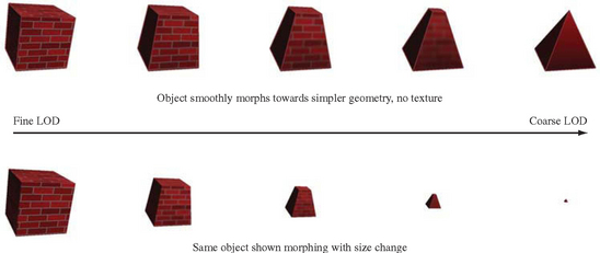
This technique doesn’t incur pixel fill overhead, since the object is always drawn once. It does require a more sophisticated modeling of objects in order to parameterize their geometry and textures. This can be a nontrivial exercise for complex models, although there is more support for such features in current modeling systems. Also, morphing requires extra computations within the application to compute the new vertex positions, so there is a trade-off of processing in the rendering pipeline for some extra processing on the CPU during transitions.
16.5 Visualizing Surface Orientation
Styling and analysis applications often provide tools to help visualize surface curvature. In addition to aesthetic properties, surface curvature can also affect the manufacturability of a particular design. Not only the intrinsic surface curvature, but the curvature relative to a particular coordinate system can determine the manufacturability of an object. For example, some manufacturing processes may be more efficient if horizontally oriented surfaces are maximized, whereas others may require vertically oriented ones (or some other constraint). Bailey and Clark (Bailey, 1997) describe a manufacturing process in which the object is constructed by vertically stacking (laminating) paper cutouts corresponding to horizontal cross sections of the object. This particular manufacturing process produces better results when the vertical slope (gradient) of the surface is greater than some threshold.
Bailey and Clark describe a method using 1D texture maps to encode the vertical slope of an object as a color ramp. The colors on the object’s surfaces represent the vertical slope of the surface relative to the current orientation. Since the surface colors dynamically display the relative slope as the object’s orientation is modified, a (human) operator can interactively search for the orientation that promises the best manufacturability.
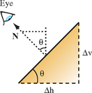
For simplicity, assume a coordinate space for surface normals with the z axis perpendicular to the way the paper sheets are stacked. If the object’s surface normals are transformed to this coordinate space, the contour line density, d, is a function of the z component of the surface normal. Figure 16.5 shows a simplified surface with normal vector N and slope angle θ and the similar triangles relationship formed with the second triangle with sides N and Nz,
where k is the (constant) paper layer thickness (in practice, approximately 0.0042 inches).
The possible range of density values, based on known manufacturing rules, can be color-coded as a red-yellow-green spectrum (using an HSV color space), and these values can in turn be mapped to the range of Nz values. For their particular case, Bailey and Clark found that a density below 100/inch causes problems for the manufacturing process. Therefore, the 1D texture is set up to map a density below 100 to red.
Typically, per-vertex surface normals are passed to OpenGL using glNormal3f calls, and such normals are used for lighting. For this rendering technique, however, the normalized per-vertex surface normal is passed to glTexCoord3f to serve as a 3D texture coordinate. The texture matrix is used to rotate the per-vertex surface normal to match the assumed coordinate space, where the z axis is perpendicular to the paper faces. A unit normal has an Nz component varying from [−1, 1], so the rotated Nz component must be transformed to the [0, 1] texture coordinate range and swizzled to the s coordinate for indexing the 1D texture. The rotation and scale and bias transformations are concatenated as
The composition of the rotation and scale and bias matrices can be computed by loading the scale and bias transform into the texture matrix first, followed by glRotate to incorporate the rotation. Once the 1D texture is loaded and enabled, the surface colors will reflect the current manufacturing orientation stored in the texture matrix. To rerender the model with a different orientation for the manufacturing process, the rotation component in the texture matrix must be adjusted to match the new orientation.
Note that there is no way to normalize a texture coordinate in the way that the OpenGL fixed-function pipeline supports GL_NORMALIZE for normalizing normals passed to glNormal3f. If rendering the model involves modelview matrix changes, such as different modeling transformations, these modelview matrix changes must also be incorporated into the texture matrix by multiplying the texture matrix by the inverse transpose of the modeling transformation.
OpenGL 1.3 alleviates both of these problems with the GL_NORMAL_MAP texture coordinate generation function. If the implementation supports this functionality, the normal vector can be transferred to the pipeline as a regular normal vector and then transferred to the texture coordinate pipeline using the texture generation function. Since the normal map function uses the eye-space normal vector, it includes any modeling transformations in effect. However, since the modelview transformation includes the viewing transformation, too, the inverse of this transformation should be included in the texture matrix.
This technique was designed to solve a particular manufacturing problem, but the ideas can be generalized. Surface normal vectors contain information about the surface gradient at that point. Various functions of the gradient can be color-coded and mapped to the surface geometry to provide additional information. The most general form of the encoding can use cube environment maps to create an arbitrary function of a 3D surface normal.
16.6 Visualizing Surface Curvature
Industrial designers are often concerned as much with how the shape of a surface reflects light as the overall shape of the surface. In many situations it is useful to render object surfaces with lighting models that provide information about surface reflection. One of the most useful techniques to simulate more realistic reflection is to use reflection mapping techniques. The sphere mapping, dual paraboloid, and cube mapping techniques described in Section 17.3 can all be used to varying degrees to realistically simulate surface reflection from a general environment.
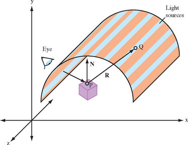
In some styling applications, simulating synthetic environments can provide useful aesthetic insights. One such environment consists of a hemi-cylindrical room with an array of regularly spaced linear light sources (fluorescent lamps) illuminating the object. The object is placed on a turntable and can be rotated relative to the orientation of the light sources. The way the surfaces reflect the array of light sources provides intuitive information regarding how the surface will appear in more general environments.
The environment can be approximated as an object enclosed in a cylinder with the light sources placed around the cylinder boundary, aligned with the longitudinal axis (as shown in Figure 16.6). The symmetry in the cylinder allows the use of a cylinder reflection mapping technique. Cylinder mapping techniques parameterize the texture map along two dimensions, θ, l, where θ is the rotation around the circumference of the cylinder and l is the distance along the cylinder’s longitudinal axis. The reflection mapping technique computes the eye reflection vector about the surface normal and the intersection of this reflection vector with the cylindrical map. Given a point P, reflection vector R and cylinder of radius r, with longitudinal axis parallel to the z axis, the point of intersection Q is P + kR, with the constraint ![]() . This results in the quadratic equation
. This results in the quadratic equation
with solution
With k determined, the larger (positive) solution is chosen, and used to calculate Q. The x and y components of Q are used to determine the angle, θ, in the x − y plane that the intersection makes with the x axis, tan θ = Qy/Qx. The parametric value l is Qz.
Since each light source extends from one end of the room to the other, the texture map does not vary with the l parameter, so the 2D cylinder map can be simplified to a 1D texture mapping θ to the s coordinate. To map the full range of angles [−π, π] to the [0, 1] texture coordinates, the mapping s = [atan(Qy/Qx)/π + 1]/2 is used. A luminance map can be used for the 1D texture map, using regularly spaced 1.0 values against 0.0 background values. The texture mapping can result in significant magnification of the texture image, so better results can be obtained using a high-resolution texture image. Similarly, finer tessellations of the model geometry reduces errors in the interpolation of the angle θ across the polygon faces.
To render using the technique, the s texture coordinate must be computed for each vertex in the model. Each time the eye position changes, the texture coordinates must be recomputed. If available, a vertex program can be used to perform the computation in the transformation pipeline.
16.7 Line Rendering Techniques
Many design applications provide an option to display models using some form of wireframe rendering using lines rather than filled polygons. Line renderings may be generated considerably faster if the application is fill limited, line renderings may be used to provide additional insight since geometry that is normally occluded may be visible in a line rendered scene. Line renderings can also provide a visual measure of the complexity of the model geometry. If all of the edges of each primitive are drawn, the viewer is given an indication of the number of polygons in the model. There are a number of useful line rendering variations, such as hidden line removal and silhouette edges, described in the following sections.
16.7.1 Wireframe Models
To draw a polygonal model in wireframe, there are several methods available, ordered from least to most efficient to render.
1. Draw the model as polygons in line mode using glBegin(GL_POLYGON) and glPolygonMode(GL_FRONT_AND_BACK, GL_LINE).
This method is the simplest if the application already displays the model as a shaded solid, since it involves a single mode change. However, it is likely to be significantly slower than the other methods because more processing usually occurs for polygons than for lines and because every edge that is common to two polygons will be drawn twice. This method is undesirable when using antialiased lines as well, since lines drawn twice will be brighter than any lines drawn just once. The double-edge problem can be eliminated by using an edge flag to remove one of the lines at a common edge. However, to use edge flags the application must keep track of which vertices are part of common edges.
2. Draw the polygons as line loops using glBegin(GL_LINE_LOOP).
This method is almost as simple as the first, requiring only a change to each glBegin call. However, except for possibly eliminating the extra processing required for polygons it has all of the other undesirable features as well. Edge flags cannot be used to eliminate the double edge drawing problem.
3. Extract the edges from the model and draw as independent lines using glBegin(GL_LINES).
This method is more work than the previous two because each edge must be identified and all duplicates removed. However, the extra work need only be done once and the resulting model will be drawn much faster.
4. Extract the edges from the model and connect as many as possible into long line strips using glBegin(GL_LINE_STRIP).
For just a little bit more effort than the GL_LINES method, lines sharing common endpoints can be connected into larger line strips. This has the advantage of requiring less storage, less data transfer bandwidth, and makes most efficient use of any line drawing hardware.
When choosing amongst these alternative methods there are some additional factors to consider. One important consideration is the choice of polygonal primitives used in the model. Independent triangles, quads, and polygons work correctly with edge flags, whereas triangle strips, triangle fans, and quad strips do not. Therefore, algorithms that use edge flags to avoid showing interior edges or double-stroking shared edges will not work correctly with connected primitives. Since connected primitives are generally more efficient than independent primitives, they are the preferred choice whenever possible. This means that the latter two explicit edge drawing algorithms are a better choice.
Conversely, glPolygonMode provides processing options that are important to several algorithms; both face culling and depth offsetting can be applied to polygons rendered as lines, but not to line primitives.
16.7.2 Hidden Lines
This section describes techniques to draw wireframe objects with their hidden lines removed or drawn in a style different from the ones that are visible. This technique can clarify complex line drawings of objects, and improve their appearance (Herrell, 1995; Attarwala, 1988).
The algorithm assumes that the object is composed of polygons. The algorithm first renders the object as polygons, and then in the second pass it renders the polygon edges as lines. During the first pass, only the depth buffer is updated. During the second pass, the depth buffer only allows edges that are not obscured by the object’s polygons to be rendered, leaving the previous content of the framebuffer undisturbed everywhere an edge is not drawn. The algorithm is as follows:
1. Disable writing to the color buffer with glColorMask.
2. Set the depth function to GL_LEQUAL.
3. Enable depth testing with glEnable(GL_DEPTH_TEST).
4. Render the object as polygons.
5. Enable writing to the color buffer.
6. Render the object as edges using one of the methods described in Section 16.7.1.
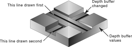
Since the pixels at the edges of primitives rendered as polygons and the pixels from the edges rendered as lines have depth values that are numerically close, depth rasterization artifacts from quantization errors may result. These are manifested as pixel dropouts in the lines wherever the depth value of a line pixel is greater than the polygon edge pixel. Using GL_LEQUAL eliminates some of the problems, but for best results the lines should be offset from the polygons using either glPolygonOffset or glDepthRange (described in more detail shortly).
The stencil buffer may be used to avoid the depth-buffering artifacts for convex objects drawn using non-antialiased (jaggy) lines all of one color. The following technique uses the stencil buffer to create a mask where all lines are (both hidden and visible). Then it uses the stencil function to prevent the polygon rendering from updating the depth buffer where the stencil values have been set. When the visible lines are rendered, there is no depth value conflict, since the polygons never touched those pixels. The modified algorithm is as follows:
1. Disable writing to the color buffer with glColorMask.
2. Disable depth testing: glDisable(GL_DEPTH_TEST).
3. Enable stenciling: glEnable(GL_STENCIL_TEST).
5. Set the stencil buffer to set the stencil values to 1 where pixels are drawn: glStencilFunc(GL_ALWAYS, 1, 1) and glStencilOp(GL_REPLACE, GL_REPLACE GL_REPLACE).
6. Render the object as edges.
7. Use the stencil buffer to mask out pixels where the stencil value is 1: glStencilFunc(GL_EQUAL, 1, 1) and glStencilOp(GL_KEEP, GL_KEEP, GL_KEEP).
8. Render the object as polygons.
9. Disable stenciling: glDisable(GL_STENCIL_TEST).
Variants of this algorithm may be applied to each convex part of an object, or, if the topology of the object is not known, to each individual polygon to render well-behaved hidden line images.
Instead of removing hidden lines, sometimes it’s desirable to render them with a different color or pattern. This can be done with a modification of the algorithm:
1. Change the depth function to GL_LEQUAL.
2. Leave the color depth buffer enabled for writing.
3. Set the color and/or pattern for the hidden lines.
4. Render the object as edges.
5. Disable writing to the color buffer.
6. Render the object as polygons.
7. Set the color and/or pattern for the visible lines.
8. Render the object as edges using one of the methods described in Section 16.7.1.
In this technique, all edges are drawn twice: first with the hidden line pattern, then with the visible one. Rendering the object as polygons updates the depth buffer, preventing the second pass of line drawing from affecting the hidden lines.
16.7.3 Polygon Offset
To enhance the preceding methods, the glPolygonOffset command can be used to move the lines and polygons relative to each other. If the edges are drawn as lines using polygon mode, glEnable(GL_POLYGON_OFFSET_LINE) can be used to offset the lines in front of the polygons. If a faster version of line drawing is used (as described in Section 16.7.1), glEnable(GL_POLYGON_OFFSET_FILL) can be used to move the polygon surfaces behind the lines. If maintaining correct depth buffer values is necessary for later processing, surface offsets may not be an option and the application should use line offsets instead.
Polygon offset is designed to provide greater offsets for polygons viewed more edge-on than for polygons that are flatter (more parallel) relative to the screen. A single constant value may not work for all polygons, since variations resulting from depth interpolation inaccuracies during rasterization are related to the way depth values change between fragments. The depth change is the z slope of the primitive relative to window-space x and y. The depth offset is computed as ow = factor * m + r * units, where  · The value of m is often approximated with the maximum of the absolute value of the x and y partial derivatives (slopes), since this can be computed more efficiently. The maximum slope value is computed for each polygon and is scaled by factor. A constant bias is added to deal with polygons that have very small slopes. When polygon offset was promoted from an extension to a core feature (OpenGL 1.1), the bias value was changed from an implementation-dependent value to a normalized scaling factor, units, in the range [0, 1]. This value is scaled by the implementation-dependent depth buffer minimum resolvable difference value, r, to produce the final value. This minimum resolvable difference value reflects the precision of the rasterization system and depth buffer storage. For a simple n-bit depth buffer, the value is 2−n, but for implementations that use compressed depth representations the derivation of the value is more complicated.
Since the slope offset must be computed separately for each polygon, the extra processing can slow down rendering. Once the parameters have been tuned for a particular OpenGL implementation, however, the same unmodified code should work well on other implementations.
16.7.4 Depth Range
An effect similar to the constant term of polygon offset can be achieved using glDepthRange with no performance penalty. This is done by displacing the near value from 0.0 by a small amount, ε, while setting the far value to 1.0 for all surface drawing. Then when the edges are drawn the near value is set to 0.0 and the far value is displaced by the same amount. Since the NDC depth value, zd, is transformed to window coordinates as
surfaces drawn with a near value of n + ε are displaced by
and lines with a far value of f−ε are displaced by
The resulting relative displacement between an edge and surface pixel is ε. Unlike the polygon offset bias, the depth range offset is not scaled by the implementation-specific minimum resolvable depth difference. This means that the application must determine the offset value empirically and that it may vary between different OpenGL implementations. Values typically start at approximately 0.00001. Since there is no slope-proportionate term, the value may need to be significantly larger to avoid artifacts with polygons that are nearly edge on.
16.7.5 Haloed Lines
Haloing lines can make it easier to understand a wireframe drawing. Lines that pass behind other lines stop short before passing behind, making it clearer which line is in front of the other.
Haloed lines can be drawn using the depth buffer. The technique uses two passes. The first pass disables updates to the color buffer, updating only the content of the depth buffer. The line width is set to be greater than the normal line width and the lines are rendered. This width determines the extent of the halos. In the second pass, the normal line width is reinstated, color buffer updates are enabled, and the lines are rendered a second time. Each line will be bordered on both sides by a wider “invisible line” in the depth buffer. This wider line will mask other lines that pass beneath it, as shown in Figure 16.7 The algorithm works for antialiased lines, too. The mask lines should be drawn as aliased lines and be as least as wide as the footprint of the antialiased lines.
1. Disable writing to the color buffer.
2. Enable the depth buffer for writing.
6. Enable writing to the color buffer.
This method will not work where multiple lines with the same depth meet. Instead of connecting, all of the lines will be “blocked” by the last wide line drawn. There can also be depth buffer rasterization problems when the wide line depth values are changed by another wide line crossing it. This effect becomes more pronounced if the narrow lines are widened to improve image clarity.
If the lines are drawn using polygon mode, the problems can be alleviated by using polygon offset to move narrower visible lines in front of the wider obscuring lines. The minimum offset should be used to avoid lines from one surface of the object “popping through” the lines of an another surface separated by only a small depth value.
If the vertices of the object’s faces are oriented to allow face culling, it can be used to sort the object surfaces and allow a more robust technique: the lines of the object’s back faces are drawn, obscuring wide lines of the front face are drawn, and finally the narrow lines of the front face are drawn. No special depth buffer techniques are needed.
1. Cull the front faces of the object.
3. Cull the back faces of the object.
Since the depth buffer isn’t needed, there are no depth rasterization problems. The back-face culling technique is fast and works well. However, it is not general since it doesn’t work for multiple obscuring or intersecting objects.
16.7.6 Silhouette Edges
Sometimes it can be useful for highlighting purposes to draw a silhouette edge around a complex object. A silhouette edge defines the outer boundaries of the object with respect to the viewer (as shown in Figure 16.8).

The stencil buffer can be used to render a silhouette edge around an object. With this technique, the application can render either the silhouette alone or the object with a silhouette around it (Rustagi, 1989).
The object is drawn four times, each time displaced by one pixel in the x or y direction. This offset must be applied to the window coordinates. An easy way to do this is to change the viewport coordinates each time, changing the viewport origin. The color and depth values are turned off, so only the stencil buffer is affected. Scissor testing can be used to avoid drawing outside the original viewport.
Every time the object covers a pixel, it increments the pixel’s stencil value. When the four passes have been completed, the perimeter pixels of the object will have stencil values of 2 or 3. The interior will have values of 4, and all pixels surrounding the object exterior will have values of 0 or 1. A final rendering pass that masks everything but pixels with stencil values of 2 or 3 produces the silhouette. The steps in the algorithm are as follows:
1. Render the object (skip this step if only the silhouette is needed).
2. Clear the stencil buffer to zero.
3. Disable color and depth buffer updates using glColorMask.
4. Set the stencil function to always pass, and set the stencil operation to increment.
5. Translate the object by +1 pixel in y, using glViewport and render the object.
6. Translate the object by −2 pixels in y, using glViewport and render the object.
7. Translate by +1 pixel x and +1 pixel in y and render the object.
8. Translate by −2 pixels in x and render the object.
9. Translate by +1 pixel in x, bringing the viewport back to the original position.
10. Enable color and depth buffer updates.
11. Set the stencil function to pass if the stencil value is 2 or 3. Since the possible values range from 0 to 4, the stencil function can pass if stencil bit 1 is set (counting from 0).
12. Render a rectangle that covers the screen-space area of the object, or the size of the viewport to render the silhouette.
One of the bigger drawbacks of this image-space algorithm is that it takes a large number of drawing passes to generate the edges. A somewhat more efficient algorithm suggested by Akeley (1998) is to use glPolygonOffset to create an offset depth image and then draw the polygons using the line polygon mode. The stencil buffer is again used to count the number of times each pixel is written. However, instead of counting the absolute number of writes to a pixel the stencil value is inverted on each write. The resulting stencil buffer will have a value of 1 wherever a pixel has been drawn an odd number of times. This ensures that lines drawn at the shared edges of polygon faces have stencil values of zero, since the lines will be drawn twice (assuming edge flags are not used). While this algorithm is a little more approximate than the previous algorithm, it only requires two passes through the geometry.
The algorithm is sensitive to the quality of the line rasterization algorithm used by the OpenGL implementation. In particular, if the line from p0 to p1 rasterizes differently from the line drawn from p1 to p0 by more than just the pixels at the endpoints, artifacts will appear along the shared edges of polygons.
The faster algorithm does not generate quite the same result as the first algorithm because it counts even and odd transitions and relies on the depth image to ensure that other nonvisible surfaces do not interfere with the stencil count. The differences arise in that boundary edges within one object that are in front of another object will be rendered as part of the silhouette image. By boundary edges we mean the true edges of the modeled geometry, but not the interior shared-face edges. In many cases this artifact is useful, as silhouette edges by themselves often do not provide sufficient information about the shape of objects. It is possible to combine the algorithm for drawing silhouettes with an additional step in which all of the boundary edges of the geometry are drawn as lines. This produces a hidden line drawing displaying boundary edges plus silhouette edges, as shown in Figure 16.8. The steps of the combined algorithm are as follows:
1. Clear the depth and color buffers and clear the stencil buffer to zero.
2. Disable color buffer writes.
3. Draw the depth buffered geometry using glPolygonOffset to offset the object surfaces toward the far clipping plane.
4. Disable writing to the depth buffer and glPolygonOffset.
5. Set the stencil function to always pass and set the stencil operation to invert.
7. Draw the geometry as lines using glPolygonMode.
8. Enable writes to the color buffer, disable face culling.
9. Set the stencil function to pass if the stencil value is 1.
10. Render a rectangle that fills the entire window to produce the silhouette image.
Since the algorithm uses an offset depth image, it is susceptible to minor artifacts from the interaction of the lines and the depth image similar to those present when using glPolygonOffset for hidden line drawings. Since the algorithm mixes lines drawn in polygon mode with line primitives, the surfaces must be offset rather than the lines. This means that the content of the depth buffer will be offset from the true geometry and may need to be reestablished for later processing.
16.7.7 Preventing Antialiasing Artifacts
When drawing a series of wide smoothed lines that overlap, such as an outline composed of a GL_LINE_LOOP, more than one fragment may be produced for a given pixel. Since smooth line rendering uses framebuffer blending, this may cause the pixel to appear brighter or darker than expected where fragments overlap.
The stencil buffer can be used to allow only a single fragment to update the pixel. When multiple fragments update a pixel, the one chosen depends on the drawing order. Ideally the fragment with the largest alpha value should be retained rather than one at random. A combination of the stencil test and alpha test can be used to pass only the fragments that have the largest alpha, and therefore contribute the most color to a pixel. Repeatedly drawing and applying alpha test to pass fragments with decreasing alpha, while using the stencil buffer to mark where fragments previously passed, results in a brute-force algorithm that has the effect of sorting fragments by alpha value.
1. Clear the stencil buffer and enable stencil testing.
2. Set the stencil function to test for not equal: glStencilFunc(GL_NOTEQUAL, 1, 0×ff).
3. Set the stencil operation to replace stencil values that pass the stencil test and depth test and keep the others.
4. Enable line smoothing and blending.
6. Loop over alpha reference values from 1.0 – step to 0, setting the alpha function to pass for alpha greater than the reference value and draw the lines. The number of passes is determined by step.
Speed can be traded for quality by increasing the step size or terminating the loop at a larger threshold value. A step of 0.02 results in 50 passes and very accurate rendering. However, good results can still be achieved with 10 or fewer passes by favoring alpha values closer to 1.0 or increasing the step size as alpha approaches 0. At the opposite extreme, it is possible to iterate through every possible alpha value, and pass only the fragments that match each specific one, using step = 1/2GL_ALPHA_BITS.
16.7.8 End Caps on Wide Lines
If wide lines form a loop, such as a silhouette edge or the outline of a polygon, it may be necessary to fill regions where one line ends and another begins to give the appearance of a rounded joint. Smooth wide points can be drawn at the ends of the line segments to form an end cap. The preceding overlap algorithm can be used to avoid blending problems where the point and line overlap.
16.8 Coplanar Polygons and Decaling
Using stenciling to control pixels drawn from a particular primitive can help solve important problems, such as the following:
Values are written to the stencil buffer to create a mask for the area to be decaled. Then this stencil mask is used to control two separate draw steps: one for the decaled region and one for the rest of the polygon.
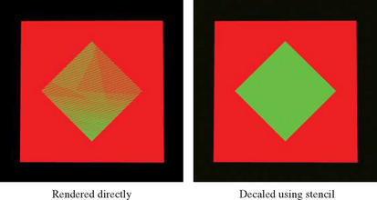
A useful example that illustrates the technique is rendering coplanar polygons. If one polygon must be rendered directly on top of another (runway markings, for example). The depth buffer cannot be relied upon to produce a clean separation between the two. This is due to the quantization of the depth buffer. Since the polygons have different vertices, the rendering algorithms can produce z values that are rounded to the wrong depth buffer value, so some pixels of the back polygon may show through the front polygon (Section 6.1.2). In an application with a high frame rate, this results in a shimmering mixture of pixels from both polygons, commonly called “z-fighting.” An example is shown in Figure 16.9.
To solve this problem, the closer polygons are drawn with the depth test disabled, on the same pixels covered by the farthest polygons. It appears that the closer polygons are “decaled” on the farther polygons. Decaled polygons can be drawn via the following steps:
1. Turn on stenciling: glEnable(GL_STENCIL_TEST).
2. Set stencil function to always pass: glStencilFunc(GL_ALWAYS, 1, 1).
3. Set stencil op to set 1 if depth test passes: 0 if it fails: glStencilOp(GL_KEEP, GL_ZERO, GL_REPLACE).
5. Set stencil function to pass when stencil is 1: glStencilFunc(GL_EQUAL, 1, 1).
6. Disable writes to stencil buffer: glStencilMask(GL_FALSE).
The stencil buffer does not have to be cleared to an initial value; the stencil values are initialized as a side effect of writing the base polygon. Stencil values will be 1 where the base polygon was successfully written into the framebuffer and 0 where the base polygon generated fragments that failed the depth test. The stencil buffer becomes a mask, ensuring that the decal polygon can only affect the pixels that were touched by the base polygon. This is important if there are other primitives partially obscuring the base polygon and decal polygons.
There are a few limitations to this technique. First, it assumes that the decal polygon does not extend beyond the edge of the base polygon. If it does, the entire stencil buffer must be cleared before drawing the base polygon. This is expensive on some OpenGL implementations. If the base polygon is redrawn with the stencil operations set to zero out the stencil after drawing each decaled polygon, the entire stencil buffer only needs to be cleared once. This is true regardless of the number of decaled polygons.
Second, if the screen extents of multiple base polygons being decaled overlap, the decal process must be performed for one base polygon and its decals before proceeding to another. This is an important consideration if the application collects and then sorts geometry based on its graphics state, because the rendering order of geometry may be changed as a result of the sort.
This process can be extended to allow for a number of overlapping decal polygons, with the number of decals limited by the number of stencil bits available for the framebuffer configuration. Note that the decals do not have to be sorted. The procedure is similar to the previous algorithm, with the following extensions.
A stencil bit is assigned for each decal and the base polygon. The lower the number, the higher the priority of the polygon. The base polygon is rendered as before, except instead of setting its stencil value to one, it is set to the largest priority number. For example, if there are three decal layers the base polygon has a value of 8.
When a decal polygon is rendered, it is only drawn if the decal’s priority number is lower than the pixels it is trying to change. For example, if the decal’s priority number is 1 it is able to draw over every other decal and the base polygon using glStencilFunc (GL_LESS, 1, 0) and glStencilOp(GL_KEEP, GL_REPLACE, GL_REPLACE).
Decals with the lower priority numbers are drawn on top of decals with higher ones. Since the region not covered by the base polygon is zero, no decals can write to it. Multiple decals can be drawn at the same priority level. If they overlap, however, the last one drawn will overlap the previous ones at the same priority level.
Multiple textures can be drawn onto a polygon using a similar technique. Instead of writing decal polygons, the same polygon is drawn with each subsequent texture and an alpha value to blend the old pixel color and the new pixel color together.
16.9 Capping Clipped Solids
When working with solid objects it is often useful to clip the object against a plane and observe the cross section. OpenGL’s application-defined clipping planes (sometimes called model clip planes) allow an application to clip the scene by a plane. The stencil buffer provides an easy method for adding a “cap” to objects that are intersected by the clipping plane. A capping polygon is embedded in the clipping plane and the stencil buffer is used to trim the polygon to the interior of the solid.
If some care is taken when modeling the object, solids that have a depth complexity greater than 2 (concave or shelled objects) and less than the maximum value of the stencil buffer can be rendered. Object surface polygons must have their vertices ordered so that they face away from the interior for face culling purposes.
The stencil buffer, color buffer, and depth buffer are cleared, and color buffer writes are disabled. The capping polygon is rendered into the depth buffer, and then depth buffer writes are disabled. The stencil operation is set to increment the stencil value where the depth test passes, and the model is drawn with glCullFace(GL_BACK). The stencil operation is then set to decrement the stencil value where the depth test passes, and the model is drawn with glCullFace(GL_FRONT).
At this point, the stencil buffer is 1 wherever the clipping plane is enclosed by the front-facing and back-facing surfaces of the object. The depth buffer is cleared, color buffer writes are enabled, and the polygon representing the clipping plane is now drawn using whatever material properties are desired, with the stencil function set to GL_EQUAL and the reference value set to 1. This draws the color and depth values of the cap into the framebuffer only where the stencil values equal 1. Finally, stenciling is disabled, the OpenGL clipping plane is applied, and the clipped object is drawn with color and depth enabled.
16.10 Constructive Solid Geometry
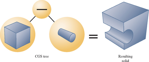
Constructive solid geometry (CSG) models are constructed through the intersection (∩), union (∪), and subtraction (–) of solid objects, some of which may be CSG objects themselves (Goldfeather, 1986). The tree formed by the binary CSG operators and their operands is known as the CSG tree. Figure 16.10 shows an example of a CSG tree and the resulting model.
The representation used in CSG for solid objects varies, but we will consider a solid to be a collection of polygons forming a closed volume. Solid, primitive, and object are used here to mean the same thing.
CSG objects have traditionally been rendered through the use of raycasting, (which is slow) or through the construction of a boundary representation (B-rep). B-reps vary in construction, but are generally defined as a set of polygons that form the surface of the result of the CSG tree. One method of generating a B-rep is to take the polygons forming the surface of each primitive and trim away the polygons (or portions thereof) that do not satisfy the CSG operations. B-rep models are typically generated once and then manipulated as a static model because they are slow to generate.
Drawing a CSG model using stenciling usually requires drawing more polygons than a B-rep would contain for the same model. Enabling stencil itself also may reduce performance. Nonetheless, some portions of a CSG tree may be interactively manipulated using stenciling if the remainder of the tree is cached as a B-rep.
The algorithm presented here is from a paper (Wiegand, 1996) describing a GL-independent method for using stenciling in a CSG modeling system for fast interactive updates. The technique can also process concave solids, the complexity of which is limited by the number of stencil planes available.
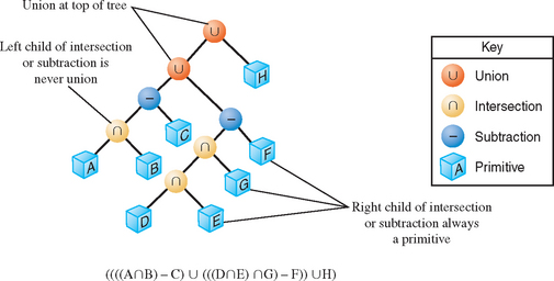
The algorithm presented here assumes that the CSG tree is in “normal” form. A tree is in normal form when all intersection and subtraction operators have a left subtree that contains no union operators and a right subtree that is simply a primitive (a set of polygons representing a single solid object). All union operators are pushed toward the root, and all intersection and subtraction operators are pushed toward the leaves. For example, (((A ∩ B) − C) ∪ (((D ∩ E) ∩ G) − F)) ∪ H is in normal form; Figure 16.11 illustrates the structure of that tree and the characteristics of a tree in this form.
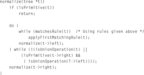
A CSG tree can be converted to normal form by repeatedly applying the following set of production rules to the tree and then its subtrees.
2. X ∩ (Y ∪ Z) * (X ∩ Y) ∪ (X ∩ Z)
3. X − (Y ∩ Z) → (X − Y) ∪ (X − Z)
5. X − (Y − Z) → (X − Y) ∪ (X ∩ Z)
X, Y, and Z here match either primitives or subtrees. The algorithm used to apply the production rules to the CSG tree follows.
CSG subtrees rooted by the intersection or subtraction operators may be pruned at each step in the normalization process using the following two rules.
1. If T is an intersection and not intersects(T->left->bounds, T->right->bounds), delete T.
2. If T is a subtraction and not intersects(T->left->bounds, T->right->bounds), replace T with T->left.
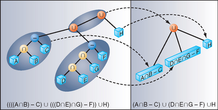
The normalized CSG tree is a binary tree, but it is important to think of the tree as a “sum of products” to understand the stencil CSG procedure.
Consider all unions as sums. Next, consider all the intersections and subtractions as products. (Subtraction is equivalent to intersection with the complement of the term to the right; for example, ![]() . Imagine all unions flattened out into a single union with multiple children. That union is the “sum.” The resulting subtrees of that union are all composed of subtractions and intersections, the right branch of those operations is always a single primitive, and the left branch is another operation or a single primitive. Consider each child subtree of the imaginary multiple union as a single expression containing all intersection and subtraction operations concatenated from the bottom up. These expressions are the “products.” For example, ((A ∩ B) − C) ∪ (((G ∩ D) − E) ∩ F) ∪ H can be thought of as (A ∩ B − C) ∪ (G ∩ D − E ∩ F) ∪ H. Figure 16.12 illustrates this process.
. Imagine all unions flattened out into a single union with multiple children. That union is the “sum.” The resulting subtrees of that union are all composed of subtractions and intersections, the right branch of those operations is always a single primitive, and the left branch is another operation or a single primitive. Consider each child subtree of the imaginary multiple union as a single expression containing all intersection and subtraction operations concatenated from the bottom up. These expressions are the “products.” For example, ((A ∩ B) − C) ∪ (((G ∩ D) − E) ∩ F) ∪ H can be thought of as (A ∩ B − C) ∪ (G ∩ D − E ∩ F) ∪ H. Figure 16.12 illustrates this process.
At this time, redundant terms can be removed from each product. Where a term subtracts itself (A − A), the entire product can be deleted. Where a term intersects itself (A ∩ A), that intersection operation can be replaced with the term itself.
All unions can be rendered simply by finding the visible surfaces of the left and right subtrees and allowing the depth test to determine the visible surface. All products can be rendered by drawing the visible surfaces of each primitive in the product and trimming those surfaces with the volumes of the other primitives in the product. For example, to render A − B the visible surfaces of A are trimmed by the complement of the volume of B, and the visible surfaces of B are trimmed by the volume of A.
The visible surfaces of a product are the front-facing surfaces of the operands of intersections and the back-facing surfaces of the right operands of subtraction. For example, in (A − B ∩ C) the visible surfaces are the front-facing surfaces of A and C and the back-facing surfaces of B.
Concave solids are processed as sets of front-facing or back-facing surfaces. The “convexity” of a solid is defined as the maximum number of pairs of front and back surfaces that can be drawn from the viewing direction. Figure 16.13 shows some examples of the convexity of objects. The nth front surface of a k-convex primitive is denoted Anf, and the nth back surface is Anb. Because a solid may vary in convexity when viewed from different directions, accurately representing the convexity of a primitive may be difficult and may involve reevaluating the CSG tree at each new view. Instead, the algorithm must be given the maximum possible convexity of a primitive; it then draws the nth visible surface by using a counter in the stencil planes.
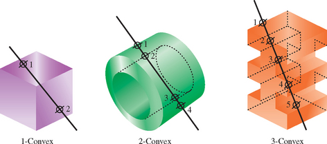
The CSG tree must be further reduced to a “sum of partial products” by converting each product to a union of products, each consisting of the product of the visible surfaces of the target primitive with the remaining terms in the product. For example, if A, B, and D are 1-convex and C is 2-convex:
Because the target term in each product has been reduced to a single front-facing or back-facing surface, the bounding volumes of that term will be a subset of the bounding volume of the original complete primitive. Once the tree is converted to partial products, the pruning process may be applied again with these subset volumes. In each resulting child subtree representing a partial product, the leftmost term is called the “target” surface, and the remaining terms on the right branches are called “trimming” primitives.
The resulting sum of partial products reduces the rendering problem to rendering each partial product correctly before drawing the union of the results. Each partial product is rendered by drawing the target surface of the partial product and then “classifying” the pixels generated by that surface with the depth values generated by each of the trimming primitives in the partial product. If pixels drawn by the trimming primitives pass the depth test an even number of times, that pixel in the target primitive is “out,” and discarded. If the count is odd, the target primitive pixel is “in,” and kept.
Because the algorithm saves depth buffer contents between each object, the number of depth saves and restores can be minimized by drawing as many of target and trimming primitives for each pass as can fit in the stencil buffer.
The algorithm uses one stencil bit (Sp) as a toggle for trimming primitive depth test passes (parity); n stencil bits for counting to the nth surface (Scount), where n is the smallest number for which 2n is larger than the maximum convexity of a current object, and as many bits as are available (Sa) to accumulate whether target pixels have to be discarded. Because Scount will require the GL_INCR operation, it must be stored contiguously in the least-significant bits of the stencil buffer. Sp and Scount are used in two separate steps, and so may share stencil bits.
For example, drawing two 5-convex primitives requires one Sp bit, three Scount bits, and two Sa bits. Because Sp and Scount are independent, the total number of stencil bits required is 5.
Once the tree is converted to a sum of partial products, the individual products are rendered. Products are grouped so that as many partial products can be rendered between depth buffer saves and restores as the stencil buffer has capacity.
For each group, color buffer writes are disabled, the contents of the depth buffer are saved, and the depth buffer is cleared. Then, every target in the group is classified against its trimming primitives. The depth buffer is then restored, and every target in the group is rendered against the trimming mask. The depth buffer save/restore can be optimized by saving and restoring only the region containing the screen-projected bounding volumes of the target surfaces.
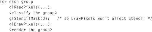
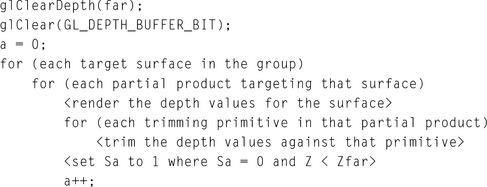
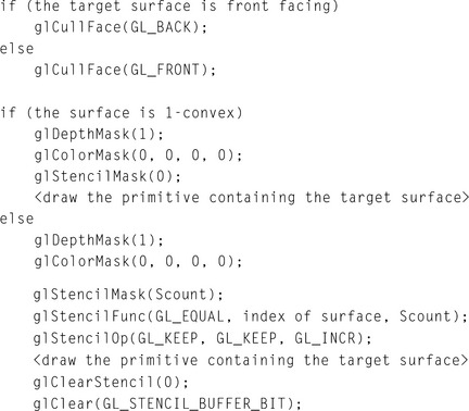
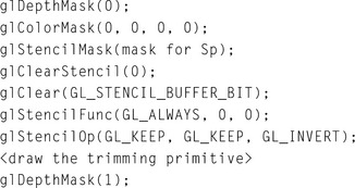
Once all the trimming primitives are rendered, the values in the depth buffer are ZF for all target pixels classified as “out.” The SA bit for that primitive is set to 1 everywhere the depth value for a pixel is not equal to ZF, and 0 otherwise.
Each target primitive in the group is finally rendered into the framebuffer with depth testing and depth writes enabled, the color buffer enabled, and the stencil function and operation set to write depth and color only where the depth test succeeds and Sa is 1. Only the pixels inside the volumes of all the trimming primitives are drawn.
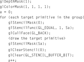
Further techniques are available for adding clipping planes (half-spaces), including more normalization rules and pruning opportunities (Wiegand, 1996). This is especially important in the case of the near clipping plane in the viewing frustum.