Compositing, Blending, and Transparency
Blending and compositing describe the task of merging together disparate collections of pixels that occupy the same locations in the output image. The basic task can be described as combining the pixels from two or more input images to form a single output image. In the general case, compositing results depend on the order in which the images are combined. Compositing is useful in many areas of computer graphics. It makes it possible to create complex scenes by rendering individual components of the scene, then combining them. The combining process itself can also add complexity and interest to images.
Semi-transparent surfaces reflect some light while allowing some light from other surfaces to pass through them. Rendering semi-transparent objects is closely related to the ideas used for compositing multiple images. The details of blending images or image elements is an almost universal building block for the rendering techniques in this book, so it is valuable to explore the operations in detail.
11.1 Combining Two Images
Given two input images A and B, an output image C can be expressed as a linear combination of the two input images:
where wa and wb are weighting factors. Constant weighting factors are used to implement simple effects such as cross fades or dissolves. For example, to cross fade from A to B, set wb in terms of wa (wb = 1 − wa) and smoothly vary wa from 0 to 1.
Blending two source images (also called elements) with constant weights isn’t selective enough to create certain effects. It’s more useful to be able to select an object or subregion from element A and a subregion from element B to produce the output composite. These subregions are arbitrary regions of pixels embedded in rectangular images. Distinguishing an arbitrary shaped subregion in an image can be done by varying the weighting function for each pixel in the image. This per-pixel weighting changes Equation 11.1 to
For convenience we will drop the indices [i, j] from this point on and assume the weights are distinct for each pixel.
To select a subregion from image A, the pixels in the subregion are given a weight of 1, while the pixels not in the subregion are given a weight of 0. This works well if the edges of the subregion are sharp and end at pixel boundaries. However, antialiased images often contain partially covered pixels at the boundary edges of objects. These boundary pixels may contain color contributions from the background, or other objects in the image in addition to the source object’s color (see the discussion of digital image representation in Chapter 4). To correct for this, the per-pixel weighting factor for these pixels is scaled to be proportional to the object’s contribution. This ensures that the contribution in the final image is the same as in the input image.
OpenGL provides this weighted per-pixel merge capability through the framebuffer blending operation. In framebuffer blending the weights are stored as part of the images themselves. Both the alpha component and the R, G, and B color components can be used as per-pixel weights or as parameters to a simple weight function, such as 1 − alpha. Framebuffer blending is often called alpha-blending since the alpha values are most often used as the weights.
11.1.1 Compositing
A common blending operation is to composite a background image, perhaps from a film or video, with a computer-generated object. In this context, the word “composite” represents a very specific image-combining operation involving images whose pixels include an α (alpha) value. The alpha value indicates either the transparency or the coverage of the object intersecting the pixel. The most common type of composite is the over operator, in which a foreground element is composited over a background element.
In traditional film technology, compositing a foreground and background image is achieved using a matte: a piece of film, aligned with the foreground image, in which areas of interest are transparent and the rest is opaque. The matte allows only the areas of interest from the foreground image to pass through. Its complement, the holdout matte, is used with digital images. A holdout matte is opaque in the areas of interest and transparent everywhere else. A digital holdout matte is the set of opacity α values for the corresponding image pixels. To combine two pixels together, the source element color is multiplied by the matte’s α value, and added to the corresponding color from the background image, scaled by 1 − α. The resulting equation is Cnew = αfCf + (1 − αf)Cb. The entire contribution of the object in the source element α is transferred to the new pixel while the background image contributes 1 − α, the remaining unclaimed portion of the new pixel.
OpenGL can be used to composite geometry against a background image by loading it into the framebuffer, then rendering the geometry on top of the background with blending enabled. Set the source and destination blend factors to GL_SRC_ALPHA and GL_ONE_MINUS_SRC_ALPHA, respectively, and assign α values of 1.0 to the rendered primitives when they are sent to the OpenGL pipeline. If the geometry is opaque and there is no antialiasing algorithm modifying the α values, the rasterized fragments will have α values of 1.0, reducing the compositing operation to a simple selection process. Without antialiasing, the computer-generated object will be composited with sharp silhouette edges, making it look less realistic than the objects in the background image that have softer edges.
The antialiasing algorithms described in Chapter 10 can be used to antialias the geometry and correct this problem. They are often a good solution, even if they are slower to generate, for compositing applications that do not need to be highly interactive during the compositing process.
Transparent objects are also represented with fractional α values. These values may come from the color assigned each vertex, the diffuse material specification, or a texture map. The α value represents the amount of light reflected by the object and 1−α represents the amount of light transmitted through the object. Transparency will be discussed later in this chapter.
11.1.2 Compositing Multiple Images
The preceding algorithm is mathematically correct for compositing an arbitrary foreground image with an opaque background. Problems arise, however, if it is used to combine several elements together. If the background image is not opaque, then the compositing equation should be:
so that the background pixel is scaled by its α value to calculate its contribution correctly. This new equation works correctly for compositing any two images together. There is a subtlety when using both this equation and the opaque-background version; while the input images are explicitly scaled by their α values as part of the compositing equation, the resulting pixel value is implicitly scaled by the new composite α value. The equation expects that the Cf and Cb inputs do not include a premultiplied alpha, but it creates a Cnew that does. The corresponding α value for the composited pixel, αnew, is αf + (1 − αf)αb. To undo the alpha scaling, Cnew should be divided by αnew.
This side effect of the compositing equation creates some confusion when discussing the compositing of multiple images, especially if the input images and intermediate images don’t consistently include a premultiplied alpha. To simplify the discussion, we use the notation ![]() to indicate a color value with a premultiplied α value
to indicate a color value with a premultiplied α value ![]() . Using this notation, the compositing equation simplifies to:
. Using this notation, the compositing equation simplifies to:
and
Now the case of compositing a foreground image with a background image where the background is itself the result of compositing two images C1 and C2 becomes:
This is the algorithm for doing back-to-front compositing, in which the background is built up by combining it with the element that lies closest to it to produce a new background image. It can be generalized to include an arbitrary number of images by expanding the innermost background term:
Notice that the OpenGL algorithm described previously for compositing geometry over a pre-existing opaque image works correctly for an arbitrary number of geometry elements rendered sequentially.
The algorithm is extended to work for a non-opaque background image in a number of ways. Either a background image whose color values are pre-multiplied by alpha is loaded, or the premultiplication is performed as part of the image-loading operation. This is done by clearing the color buffer to zero, enabling blending with GL_SRC_ALPHA, GL_ZERO source and destination blend factors, and transferring an image containing both color and α values to the framebuffer. If the OpenGL implementation supports fragment programs, then the fragment program can perform the premultiplication operation explicitly.
A sequence of compositing operations can also be performed front-to-back. Each new input image is composited under the current accumulated image. Renumbering the indices so that n becomes 0 and vice versa and expanding out the products, Equation 11.3 becomes:

To composite from front to back, each image must be multiplied by its own alpha value and the product of (1 − αk) of all preceding images. This means that the calculation used to compute the color values isn’t the same as those used to compute the intermediate weights. Considering only premultiplied alpha inputs, the intermediate result image is ![]() and the running composite weight is wj = (1 − αj)wj−1. This set of computations can be computed using OpenGL alpha blending by accumulating the running weight in the destination alpha buffer. However, this also requires separate specification of RGB color and alpha blend functions.1 If separate functions are supported, then GL_DST_ALPHA and GL_ONE are used for the RGB source and destination factors and GL_ZERO and GL_ONE_MINUS_SRC_ALPHA are used to accumulate the weights. For non-premultiplied alpha images, a fragment program or multipass algorithm is required to produce the correct result, since the incoming fragment must be weighted and multiplied by both the source and destination α values. Additionally, if separate blend functions are not supported, emulating the exact equations becomes more difficult.
and the running composite weight is wj = (1 − αj)wj−1. This set of computations can be computed using OpenGL alpha blending by accumulating the running weight in the destination alpha buffer. However, this also requires separate specification of RGB color and alpha blend functions.1 If separate functions are supported, then GL_DST_ALPHA and GL_ONE are used for the RGB source and destination factors and GL_ZERO and GL_ONE_MINUS_SRC_ALPHA are used to accumulate the weights. For non-premultiplied alpha images, a fragment program or multipass algorithm is required to produce the correct result, since the incoming fragment must be weighted and multiplied by both the source and destination α values. Additionally, if separate blend functions are not supported, emulating the exact equations becomes more difficult.
The coverage-based polygon antialiasing algorithm described in Section 10.6 also uses a front-to-back algorithm. The application sorts polygons from front to back, blending them in that order. It differs in that the source and destination weights are min(αs, 1 − αd) and 1 rather than αd and 1. Like the front-to-back compositing algorithm, as soon as the pixel is opaque, no more contributions are made to the pixel. The compositing algorithm achieves this as the running weight wj stored in destination alpha reaches zero, whereas polygon antialiasing achieves this by accumulating an approximation of the α value for the resulting pixel in destination α converging to 1. These approaches work because OpenGL defines separate blend functions for the GL_SRC_ALPHA_SATURATE source factor. For the RGB components the factor is min(αs, 1 − αd); however, for the α component the blend factor is 1. This means that the value computed in destination α is αj = αs + αj − 1 where αs is the incoming source α value. So, with the saturate blend function, the destination α value increases while the contribution of each sample decreases.
The principle reason for the different blend functions is that both the back-to-front and front-to-back composition algorithms make a uniform opacity assumption. This means the material reflecting or transmitting light in a pixel is uniformly distributed throughout the pixel. In the absence of extra knowledge regarding how the geometry fragments are distributed within the pixel, every sub-area of the pixel is assumed to contain an equal distribution of geometry and empty space.
In the polygon antialiasing algorithm, the uniform opacity assumption is not appropriate for polygons that share a common edge. In those situations, the different parts of the polygon don’t overlap, and rendering with the uniform assumption causes the polygons under-contributing to the pixel, resulting in artifacts at the shared edges. The source fragments generated from polygon antialiasing also need to be weighted by the source α value (i.e., premultiplied). The saturate function represents a reasonable compromise between weighting by the source alpha when it is small and weighting by the unclaimed part of the pixel when its value is small. The algorithm effectively implements a complementary opacity assumption where the geometry for two fragments within the same pixel are assumed to not overlap and are simply accumulated. Accumulation is assumed to continue until the pixel is completely covered. This results in correct rendering for shared edges, but algorithms that use the uniform opacity assumption, such as rendering transparent objects, are not blended correctly.
Note that the back-to-front algorithm accumulates the correct composite α value in the color buffer (assuming destination alpha is available), whereas this front-to-back method does not. The correct α term at each step is computed using the same equation as for the RGB components αj′ = α′j−1 +wj−1αj. The saturate function used for polygon antialiasing can be used as an approximation of the functions needed for front-to-back compositing, but it will introduce errors since it doesn’t imply uniform opacity. However, the value accumulated in destination alpha is the matching α value for the pixel.
11.1.3 Alpha Division
Both the back-to-front and front-to-back compositing algorithms (and the polygon antialiasing algorithm) compute an RGB result that has been premultiplied by the corresponding α value; in other words, ![]() is computed rather than C. Sometimes it is necessary to recover the original non-premultiplied color value. To compute this result, each color value must be divided by the corresponding α value. Only the programmable fragment pipeline supports division directly. However, a multipass algorithm can be used to approximate the result in the absence of programmability. As suggested in Section 9.3.2, a division operation can be implemented using pixel textures if they are supported.
is computed rather than C. Sometimes it is necessary to recover the original non-premultiplied color value. To compute this result, each color value must be divided by the corresponding α value. Only the programmable fragment pipeline supports division directly. However, a multipass algorithm can be used to approximate the result in the absence of programmability. As suggested in Section 9.3.2, a division operation can be implemented using pixel textures if they are supported.
11.2 Other Compositing Operators
Porter and Duff (1984) describe a number of operators that are useful for combining multiple images. In addition to over, these operators include in, out, atop, xor, and plus, as shown in Table 11.1. These operators are defined by generalizing the compositing equation for two images, A and B to
and substituting Fa and Fb with the terms from Table 11.1.
Table 11.1
| operation | Fa | Fb |
| A over B | 1 | 1−αA |
| B over A | 1−αA | 1 |
| A in B | αB | 0 |
| B in A | 0 | αA |
| A out B | 1 − αB | 0 |
| B out A | 0 | 1−αA |
| A atop B | αB | 1−αA |
| B atop A | 1−αB | αA |
| A xor B | 1−αB | 1−αA |
| A plus B | 1 | 1 |
This equation assumes that the two images A and B have been pre-multiplied by their α values. Using OpenGL, these operators are implemented using framebuffer blending, modifying the source and destination blend factors to match Fa and Fb. Assuming that the OpenGL implementation supports a destination alpha buffer with double buffering, alpha premultiplication can be incorporated by first loading the front and back buffers with the A and B images using glBlendFunc(GL_ONE, GL_ZERO) to do the premultiplication. The blending factors are then changed to match the factors from Table 11.1. glCopyPixels is used to copy image A onto image B. This simple and general method can be used to implement all of the operators. Some of them, however, may be implemented more efficiently. If the required factor from Table 11.1 is 0, for example, the image need not be premultiplied by its α value, since only its α value is required. If the factor is 1, the premultiplication by alpha can be folded into the same blend as the operator, since the 1 performs no useful work and can be replaced with a multiplication by α.
In addition to framebuffer blending, the multitexture pipeline can be used to perform similar blending and compositing operations. The combine and crossbar texture environment functions enable a number of useful equations using source operands from texture images and the source fragment. The fundamental difference is that results cannot be directly accumulated into one of the texture images. However, using the render-to-texture techniques described in Sections 5.3 and 7.5, a similar result can be achieved.
11.3 Keying and Matting
The term chroma keying has its roots in broadcast television. The principal subject is recorded against a constant color background—traditionally blue. As the video signal is displayed, the parts of the signal corresponding to the constant color are replaced with an alternate image. The resulting effect is that the principal subject appears overlayed on the alternate background image. The chroma portion of the video signal is used for the comparison, hence the name. Over time the term has been generalized. It is now known by a number of other names including color keying, blue and green screening, or just plain keying, but the basic idea remains the same. More recently the same basic idea is used, recording against a constant color background, but the keying operation has been updated to use digital compositing techniques.
Most of the aspects of compositing using blending and the α channel also apply to keying. The principal difference is that the opacity or coverage information is in one of the color channels rather than in the α channel. The first step in performing keying digitally is moving the opacity information into the alpha channel. In essence, a holdout matte is generated from the information in the color channels. Once this is done, then the alpha channel compositing algorithms can be used.
11.4 Blending Artifacts
A number of different types of artifacts may result when blending or compositing multiple images together. In this section we group the sources of errors into common classes and look at each individually.
11.4.1 Arithmetic Errors
The arithmetic operations used to blend pixels together can be a source of error in the final image. Section 3.4 discusses the use of fixed-point representation and arithmetic in the fragment processing pipeline and some of the inherent problems. When compositing a 2- or 3- image sequence, there is seldom any issue with 8-bit framebuffer arithmetic. When building up complex scenes with large numbers of compositing operations, however, poor arithmetic implementations and quantization errors from limited precision can quickly accumulate and result in visible artifacts.
A simple rule of thumb is that each multiply operation introduces at least ![]() -bit error when a 2 × n-bit product is reduced to n-bits. When performing a simple over composite the αC term may, conservatively, be in error by as much as 1 bit. With 8-bit components, this translates to roughly 0.4% error per compositing operation. After 10 compositing operations, this will be 4% error and after 100 compositing operations, 40% error. The ideal solution to the problem is to use more precision (deeper color buffer) and better arithmetic implementations. For high-quality blending, 12-bit color components provide enough precision to avoid artifacts. Repeating the 1-bit error example with 12-bit component resolution, the error changes to approximately 0.025% after each compositing operation, 0.25% after 10 operations, and 2.5% after 100 operations.
-bit error when a 2 × n-bit product is reduced to n-bits. When performing a simple over composite the αC term may, conservatively, be in error by as much as 1 bit. With 8-bit components, this translates to roughly 0.4% error per compositing operation. After 10 compositing operations, this will be 4% error and after 100 compositing operations, 40% error. The ideal solution to the problem is to use more precision (deeper color buffer) and better arithmetic implementations. For high-quality blending, 12-bit color components provide enough precision to avoid artifacts. Repeating the 1-bit error example with 12-bit component resolution, the error changes to approximately 0.025% after each compositing operation, 0.25% after 10 operations, and 2.5% after 100 operations.
11.4.2 Blending with the Accumulation Buffer
While the accumulation buffer is designed for combining multiple images with high precision, its ability to reduce compositing errors is limited. While the accumulation buffer does act as an accumulator with higher precision than found in most framebuffers, it only supports scaling by a constant value, not by a per-pixel weight such as α. This means that per-pixel scaling must still be performed using blending; only the result can be accumulated. The accumulation buffer is most effective at improving the precision of multiply-add operations, where the multiplication is by a constant. The real value of the accumulation buffer is that it can accumulate a large number of very small values, whereas the normal color buffer likely does not have enough dynamic range to represent both the end result and a single input term at the same time.
11.4.3 Approximation Errors
Another, more subtle, error can occur with the use of opacity to represent coverage at the edges of objects. The assumption with coverage values is that the background color and object color are uniformly spread across the pixel. This is only partly correct. In reality, the object occupies part of the pixel area and the background (or other objects) covers the remainder. The error in the approximation can be illustrated by compositing a source element containing an opaque object with itself. Since the objects are aligned identically and one is in front of the other, the result should be the source element itself. However, a source element pixel where α is not equal to 1 will contribute ![]() to the new pixel. The overall result is that the edges become brighter in the composite. In practice, the problem isn’t as bad as it might seem since the equal-distribution assumption is valid if there isn’t a lot of correlation between the edges in the source elements. This is one reason why the polygon antialiasing algorithm described in Section 10.6 does not use the regular compositing equations.
to the new pixel. The overall result is that the edges become brighter in the composite. In practice, the problem isn’t as bad as it might seem since the equal-distribution assumption is valid if there isn’t a lot of correlation between the edges in the source elements. This is one reason why the polygon antialiasing algorithm described in Section 10.6 does not use the regular compositing equations.
Alpha-compositing does work correctly when α is used to model transparency. If a transparent surface completely overlaps a pixel, then the α value represents the amount of light that is reflected from the surface and 1 − α represents the amount of light transmitted through the surface. The assumption that the ratios of reflected and transmitted light are constant across the area of the pixel is reasonably accurate and the correct results are obtained if a source element with a semi-transparent object is composited with itself.
11.4.4 Gamma Correction Errors
Another frequent source of error occurs when blending or compositing images with colors that are not in a linear space. Blending operators are linear and assume that the operands in the equations have a linear relationship. Images that have been gamma-corrected no longer have a linear relationship between color values. To correctly composite two gamma-corrected images, the images should first be converted back to linear space, composited, then have gamma correction re-applied. Often applications skip the linear conversion and re-gamma correction step. The amount of error introduced depends on where the input color values are on the gamma correction curve. In A Ghost in a Snowstorm (1998a), Jim Blinn analyzes the various error cases and determines that the worst errors occur with when mixing colors at opposite ends of the range, compositing white over black or black over white. The resulting worst case error can be greater than 25%.
11.5 Compositing Images with Depth
Section 11.1 discusses algorithms for compositing two images together using alpha values to control how pixels are merged. One drawback of this method is that only simple visibility information can be expressed using mattes or masks. By retaining depth information for each image pixel, the depth information can be used during the compositing operation to provide more visible surface information. With alpha-compositing, elements that occupy the same destination area rely on the alpha information and the back-to-front ordering to provide visibility information. Objects that interpenetrate must be rendered together to the same element using a hidden surface algorithm, since the back-to-front algorithm cannot correctly resolve the visible surfaces.
Depth information can greatly enhance the applicability of compositing as a technique for building up a final image from separate elements (Duff, 1985). OpenGL allows depth and color values to be read from the framebuffer using glReadPixels and saved to secondary storage for later compositing. Similarly, rectangular images of depth or color values can be independently written to the framebuffer using glDrawPixels. However, since glDrawPixels works on depth and color images one at a time, some additional work is required to perform a true 3D composite, in which the depth information is used in the visibility test.
Both color and depth images can be independently saved to memory and later drawn to the screen using glDrawPixels. This is sufficient for 2D style composites, where objects are drawn on top of each other to create the final scene. To do true 3D compositing, it is necessary to use the color and depth values simultaneously, so that depth testing can be used to determine which surfaces are obscured by others.
The stencil buffer can be used to implement true 3D compositing as a two-pass operation. The color buffer is disabled for writing, the stencil buffer is cleared, and the saved depth values are copied into the framebuffer. Depth testing is enabled, ensuring that only depth values that are closer to the original can update the depth buffer. glStencilOp is used to configure the stencil test so that the stencil buffer bit is set if the depth test passes.
The stencil buffer now contains a mask of pixels that were closer to the view than the pixels of the original image. The stencil function is changed to accomplish this masking operation, the color buffer is enabled for writing, and the color values of the saved image are drawn to the framebuffer.
This technique works because the fragment operations, in particular the depth test and the stencil test, are part of both the geometry and imaging pipelines in OpenGL. The technique is described here in more detail. It assumes that both the depth and color values of an image have been saved to system memory, and are to be composited using depth testing to an image in the framebuffer:
1. Clear the stencil buffer using glClear with GL_STENCIL_BUFFER_BIT set in the bitmask.
2. Disable the color buffer for writing with glColorMask.
3. Set stencil values to 1 when the depth test passes by calling glStencilFunc(GL_ALWAYS, 1, 1), and glStencilOp(GL_KEEP, GL_KEEP, GL_REPLACE).
4. Ensure depth testing is set; glEnable(GL_DEPTH_TEST), glDepthFunc (GL_LESS).
5. Draw the depth values to the framebuffer with glDrawPixels, using GL_DEPTH_COMPONENT for the format parameter.
6. Set the stencil buffer to test for stencil values of 1 with glStencilFunc(GL_EQUAL, 1, 1) and glStencilOp(GL_KEEP, GL_KEEP, GL_KEEP).
7. Disable the depth testing with glDisable(GL_DEPTH_TEST).
8. Draw the color values to the framebuffer with glDrawPixels, using GL_RGBA as the format parameter.
At this point, both the depth and color values will have been merged, using the depth test to control which pixels from the saved image update the framebuffer. Compositing can still be problematic when merging images with coplanar polygons.
This process can be repeated to merge multiple images. The depth values of the saved image can be manipulated by changing the values of GL_DEPTH_SCALE and GL_DEPTH_BIAS with glPixelTransfer. This technique makes it possible to squeeze the incoming image into a limited range of depth values within the scene.
11.6 Other Blending Operations
So far we have described methods that use the alpha component for weighting pixel values. OpenGL blending supports additional source and destination blend factors which can be used to implement other algorithms. A short summary of the more common operations follows.
Summing Two Images Using GL_ONE as the source and destination blend factors, the source image is added to the destination image. This operation is useful in multipass sequences to combine the results of two rendering passes.
Modulating an Image In the alpha-blending discussion, each of the color components have been weighted equally by a value in the alpha channel. Some applications require scaling the color components by different amounts depending on their relative contributions. For example, in the OpenGL lighting equation the lighting computations may produce a different result for each color channel. To reproduce the result of scaling an image by different light colors, each color component of the image must be scaled separately. This can be done using either the GL_SRC_COLOR destination or GL_DST_COLOR source factor to scale the current framebuffer contents. For example, drawing a constant-colored window-sized rectangle with GL_DST_COLOR and GL_ZERO as the source and destination factors scales the color buffer contents by the color of the rectangle.
Constant Colors The ARB imaging subset and OpenGL 1.4 support constant blending factors. These are useful to perform constant scaling operations, for example simple cross fades.
Subtraction The ARB imaging subset also supports a subtraction equation (actually both subtract and reverse subtract) in addition to the original addition operation. These allow more general purpose arithmetic to be performed in the framebuffer, most usefully as part of a multipass toolbox as described in Section 9.3.
Min/Max Arguably stretching the idea of blending a bit, the min and max functions allow per-pixel computation of the minimum and maximum values for each component for each pixel. These functions can be useful for a number of imaging operations, as described in Chapter 12.
11.7 Dissolves
A common film technique is the “dissolve”, where one image or animated sequence is replaced with another, in a smooth transition. One simple version alpha blends the two images together, fading out the first image with α and fading in the second with 1 − α. One way to think about the dissolve sequence is as a dynamic mask that changes each frame and is applied to the two target images. As discussed at the beginning of the chapter, the masks may be simple selection operations in which the pixel is selected from either the first or second image. A more general form is to take a weighted sum of the two pixels. For a simple selection operation, there are additional methods for performing it. The alpha-test fragment operation can be used to discard fragments based on their alpha value. Often dissolves are used to describe transitions between two static images, or sequences of pregenerated images. The concept can be equally well applied to sequences of images that are generated dynamically. For example, the approach can be used to dissolve between two dynamically rendered 3D scenes.
Alpha testing can be used to implement very efficient selection operations, since it discards pixels before depth and stencil testing and blending operations. One issue with using alpha testing is generating the alpha values themselves. For a dissolve the mask is usually independent and unrelated to the source image. One way to “tack on” a set of alpha values during rasterization is to use an alpha texture. A linear texture coordinate generation function is used to produce texture coordinates, indexing the texture map as a screen-space matte. To achieve the dynamic dissolve, the texture is updated each frame, either by binding different texture objects or by replacing the contents of the texture map. An alpha-texture-based technique works well when multitexture is supported since an unused texture unit may be available for the operation. The alpha-texture-based technique works with both alpha-testing or alpha-blending style algorithms.
Another option for performing masking operations is the stencil buffer. The stencil buffer can be used to implement arbitrary dissolve patterns. The alpha planes of the color buffer and the alpha function can also be used to implement this kind of dissolve, but using the stencil buffer frees up the alpha planes for motion blur, transparency, smoothing, and other effects.
The basic approach to a stencil buffer dissolve is to render two different images, using the stencil buffer to control where each image can draw to the framebuffer. This can be done very simply by defining a stencil test and associating a different reference value with each image. The stencil buffer is initialized to a value such that the stencil test will pass with one of the images’ reference values, and fail with the other. An example of a dissolve part way between two images is shown in Figure 11.1.
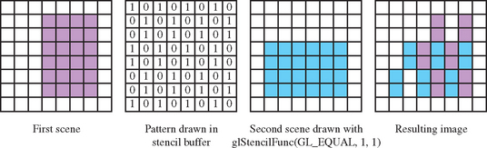
At the start of the dissolve (the first frame of the sequence), the stencil buffer is all cleared to one value, allowing only one of the images to be drawn to the framebuffer. Frame by frame, the stencil buffer is progressively changed (in an application-defined pattern) to a different value, one that passes only when compared against the second image’s reference value. As a result, more and more of the first image is replaced by the second.
Over a series of frames, the first image “dissolves” into the second under control of the evolving pattern in the stencil buffer.
Here is a step-by-step description of a dissolve.
1. Clear the stencil buffer with glClear(GL_STENCIL_BUFFER_BIT).
2. Disable writing to the color buffer, using glColorMask(GL_FALSE, GL_FALSE, GL_FALSE, GL_FALSE).
3. If the values in the depth buffer should not change, use glDepthMask(GL_FALSE).
For this example, the stencil test will always fail, setting the stencil operation to write the reference value to the stencil buffer. The application should enable stenciling before beginning to draw the dissolve pattern.
1. Turn on stenciling: glEnable(GL_STENCIL_TEST).
2. Set stencil function to always fail: glStencilFunc(GL_NEVER, 1, 1).
3. Set stencil op to write 1 on stencil test failure: glStencilOp(GL_REPLACE, GL_KEEP, GL_KEEP).
4. Write the dissolve pattern to the stencil buffer by drawing geometry or using glDrawPixels.
5. Disable writing to the stencil buffer with glStencilMask(GL_FALSE).
6. Set stencil function to pass on 0: glStencilFunc(GL_EQUAL, 0, 1).
7. Enable color buffer for writing with glColorMask(GL_TRUE, GL_TRUE, GL_TRUE, GL_TRUE).
8. If you’re depth testing, turn depth buffer writes back on with glDepthMask.
9. Draw the first image. It will only be written where the stencil buffer values are 0.
10. Change the stencil test so only values that equal 1 pass: glStencilFunc(GL_EQUAL, 1, 1).
11. Draw the second image. Only pixels with a stencil value of 1 will change.
12. Repeat the process, updating the stencil buffer so that more and more stencil values are 1. Use the dissolve pattern and redraw image 1 and 2 until the entire stencil buffer has 1’s in it and only image 2 is visible.
If each new frame’s dissolve pattern is a superset of the previous frame’s pattern, image 1 doesn’t have to be re-rendered. This is because once a pixel of image 1 is replaced with image 2, image 1 will never be redrawn there. Designing the dissolve pattern with this restriction can improve the performance of this technique.
11.8 Transparency
Accurate rendering of transparent objects is an important element of creating realistic scenes. Many objects, both natural and artificial, have some degree of transparency. Transparency is also a useful feature when visualizing the positional relationships of multiple objects. Pure transparency, unless refraction is taken into account, is straightforward. In most cases, when a transparent object is desired, what is really wanted is a partially transparent object. By definition, a partially transparent object has some degree of opacity: it is measured by the percentage of light that won’t pass through an object. Partially transparent objects don’t just block light; they also add their own color, which modifies the color of the light passing through them.
Simulating transparency is not just a useful technique in and of itself. The blending techniques used to create the most common form of transparency are also the basis of many other useful graphics algorithms. Examples include material mapping, line antialiasing, billboarding, compositing, and volume rendering. This section focuses on basic transparency techniques, with an emphasis on the effective use of blending techniques.
In computer graphics, transparent objects are modeled by creating an opaque version of a transparent object, then modifying its transparency. The opacity of an object is defined independently of its color and is expressed as a fraction between 0 and 1, where 1 means fully opaque. Sometimes the terms opacity and transparency are used inter-changably; strictly speaking, transparency is defined as 1 − opacity; a fully transparent object has an opacity of 0.
An object is made to appear transparent by rendering a weighted sum of the color of the transparent object and the color of the scene obscured by the transparent object. A fully opaque object supplies all of its color, and none from the background; a fully transparent object does the opposite. The equation for computing the output color of a transparent object, A, with opacity, oA, at a single point is:
Applying this equation properly implies that everything behind the transparent object is rendered already as Cbackground so that it is available for blending. If multiple transparent objects obscure each other, the equation is applied repeatedly. For two objects A and B (with A in front of B), the resulting color depends on the order of the transparent objects relative to the viewer. The equation becomes:
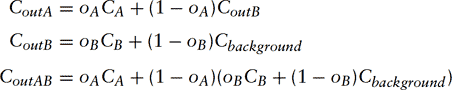
The technique for combining transparent surfaces is identical to the back-to-front compositing process described in Section 11.1. The simplest transparency model assumes that a pixel displaying the transparent object is completely covered by a transparent surface. The transparent surface transmits 1 − o of the light reflected from the objects behind it and reflects o of its own incident light. For the case in which boundary pixels are only partially covered by the transparent surface, the uniform distribution (uniform opacity) assumption described in Section 11.1.2 is combined with the transparency model.
The compositing model assumes that when a pixel is partially covered by a surface, pieces of the overlapping surface are randomly distributed across the pixel such that any subarea of the pixel contains α of the surface. The two models can be combined such that a pixel partially covered by a transparent surface can have its α and o values combined to produce a single weight, αo. Like the compositing algorithm, the combined transparency compositing process can be applied back-to-front or front-to-back with the appropriate change to the equations.
11.9 Alpha-Blended Transparency
The most common technique used to draw transparent geometry is alpha blending. This technique uses the alpha value of each fragment to represent the opacity of the object. As an object is drawn, each fragment is combined with the values in the framebuffer pixel (which is assumed to represent the background scene) using the alpha value of the fragment to represent opacity:
The resulting output color, Cfinal, is written to the frame buffer. Csrc and αsrc are the fragment source color and alpha components. Cdst is the destination color, which is already in the framebuffer. This blending equation is specified using glBlendFunc with GL_SRC_ALPHA and GL_ONE_MINUS_SRC_ALPHA as the source and destination blend factors. The alpha blending algorithm implements the general transparency formula (Equation 11.5) and is order-dependent.
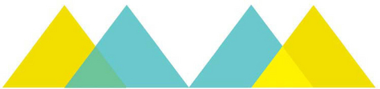
An illustration of this effect is shown in Figure 11.2, where two pairs of triangles, one pair on the left and one pair on the right, are drawn partially overlapped. Both pairs of triangles have the same colors, and both have opacities of 15. In each pair, the triangle on the left is drawn first. Note that the overlapped regions have different colors; they differ because the yellow triangle of the left pair is drawn first, while the cyan triangle is the first one drawn in the right pair.
As mentioned previously, the transparency blending equation is order-dependent, so transparent primitives drawn using alpha blending should always be drawn after all opaque primitives are drawn. If this is not done, the transparent objects won’t show the color contributions of the opaque objects behind them. Where possible, the opaque objects should be drawn with depth testing on, so that their depth relationships are correct, and so the depth buffer will contain information on the opaque objects. When drawing transparent objects in a scene that has opaque ones, turning on depth buffer testing will prevent transparent objects from being incorrectly drawn over the opaque ones that are in front of them.
Overlapping transparent objects in the scene should be sorted by depth and drawn in back-to-front order: the objects furthest from the eye are drawn first, those closest to the eye are drawn last. This forces the sequence of blending operations to be performed in the correct order.
Normal depth buffering allows a fragment to update a pixel only if the fragment is closer to the viewer than any fragment before it (assuming the depth compare function is GL_LESS). Fragments that are farther away won’t update the framebuffer. When the pixel color is entirely replaced by the fragment’s color, there is no problem with this scheme. But with blending enabled, every pixel from a transparent object affects the final color.
If transparent objects intersect, or are not drawn in back to front order, depth buffer updates will prevent some parts of the transparent objects from being drawn, producing incorrect results. To prevent this, depth buffer updates can be disabled using glDepthMask(GL_FALSE) after all the opaque objects are drawn. Note that depth testing is still active, just the depth buffer updates are disabled. As a result, the depth buffer maintains the relationship between opaque and transparent objects, but does not prevent the transparent objects from occluding each other.
In some cases, sorting transparent objects isn’t enough. There are objects, such as transparent objects that are lit, that require more processing. If the back and front faces of the object aren’t drawn in back-to-front order, the object can have an “inside out” appearance. Primitive ordering within an object is required. This can be difficult, especially if the object’s geometry wasn’t modeled with transparency in mind. Sorting of transparent objects is covered in more depth in Section 11.9.3.
If sorting transparent objects or object primitives into back-to-front order isn’t feasible, a less accurate, but order-independent blending method can be used instead. Blending is configured to use GL_ONE for the destination factor rather than GL_ONE_MINUS_SRC_ALPHA. The blending equation becomes:
This blending equation weights transparent surfaces by their opacity, but the accumulated background color is not changed. Because of this, the final result is independent of the surface drawing order. The multi-object blending equation becomes:
There is a cost in terms of accuracy with this approach; since the background color attenuation from Equation 11.5 has been eliminated, the resulting colors are too bright and have too much contribution from the background objects. It is particularly noticeable if transparent objects are drawn over a light-colored background or bright background objects.
Alpha-blended transparency sometimes suffers from the misconception that the technique requires a framebuffer with alpha channel storage. For back-to-front algorithms, the alpha value used for blended transparency comes from the fragments generated in the graphics pipeline; alpha values in the framebuffer (GL_DST_ALPHA) are not used in the blending equation, so no alpha buffer is required to store them.
11.9.1 Dynamic Object Transparency
It is common for an object’s opacity values to be configured while modeling its geometry. Such static opacity can be stored in the alpha component of the vertex colors or in per-vertex diffuse material parameters. Sometimes, though, it is useful to have dynamic control over the opacity of an object. This might be as simple as a single value that dynamically controls the transparency of the entire object. This setting is useful for fading an object in or out of a scene (see Section 16.4 for one use of this capability). If the object being controlled is simple, using a single color or set of material parameters over its entire surface, the alpha value of the diffuse material parameter or object color can be changed and sent to OpenGL before rendering the object each frame.
For complex models that use per-vertex reflectances or surface textures, a similar global control can be implemented using constant color blending instead. The ARB imaging subset provides an application-defined constant blend color that can be used as the source or destination blend factor.2 This color can be updated each frame, and used to modify the object’s alpha value with the blend value GL_CONSTANT_ALPHA for the source and GL_ONE_MINUS_CONSTANT_ALPHA for the destination blend factor.
If the imaging subset is not supported, then a similar effect can be achieved using multitexure. An additional texture unit is configured with a 1D texture containing a single component alpha ramp. The unit’s texture environment is configured to modulate the fragment color, and the unit is chained to act on the primitive after the surface texturing has been done. With this approach, the s coordinate for the additional texture unit is set to index the appropriate alpha value each time the object is drawn. This idea can be extended to provide even finer control over the transparency of an object. One such algorithm is described in Section 19.4.
11.9.2 Transparency Mapping
Because the key to alpha transparency is control of each fragment’s alpha component, OpenGL’s texture machinery is a valuable resource as it provides fine control of alpha. If texturing is enabled, the source of the alpha component is controlled by the texture’s internal format, the current texture environment function, and the texture environment’s constant color. Many intricate effects can be implemented using alpha values from textures.
A common example of texture-controlled alpha is using a texture with alpha to control the outline of a textured object. A texture map containing alpha can define an image of an object with a complex outline. Beyond the boundaries of the outline, the texel’s alpha components can be zero. The transparency of the object can be controlled on a per-texel basis by controlling the alpha components of the textures mapped on its surface.
For example, if the texture environment mode is set to GL_REPLACE (or GL_MODULATE, which is a better choice for lighted objects), textured geometry is “clipped” by the texture’s alpha components. The geometry will have “invisible” regions where the texel’s alpha components go to zero, and be partially transparent where they vary between zero and one. These regions colored with alpha values below some threshold can be removed with either alpha testing or alpha blending. Note that texturing using GL_MODULATE will only work if the alpha component of the geometry’s color is one; any other value will scale the transparency of the results. Both methods also require that blending (or alpha test) is enabled and set properly.
This technique is frequently used to draw complicated geometry using texture-mapped polygons. A tree, for example, can be rendered using an image of a tree texture mapped onto a single rectangle. The parts of the texture image representing the tree itself have an alpha value of 1; the parts of the texture outside of the tree have an alpha value of 0. This technique is often combined with billboarding (see Section 13.5), a technique in which a rectangle is turned to perpetually face the eye point.
Alpha testing (see Section 6.2.2) can be used to efficiently discard fragments with an alpha value of zero and avoid using blending, or it can be used with blending to avoid blending fragments that make no contribution. The threshold value may be set higher to retain partially transparent fragments. For example the alpha threshold can be set to 0.5 to capture half of the semi-transparent fragements, avoiding the overhead of blending while still getting acceptable results. An alternative is to use two passes with different alpha tests. In the first pass, draw the opaque fragments with depth updates enabled and transparent fragments discarded; in the second pass, draw the non-opaque parts with blending enabled and depth updates disabled. This has the advantage of avoiding blending operations for large opaque regions, at the cost of two passes.
11.9.3 Transparency Sorting
The sorting required for proper alpha transparency can be complex. Sorting is done using eye coordinates, since the back-to-front ordering of transparent objects must be done relative to the viewer. This requires the application transform geometry to eye space for sorting, then send the transparent objects in sorted order through the OpenGL pipeline.
If transparent objects interpenetrate, the individual triangles comprising each object should be sorted and drawn from back to front to avoid rendering the individual triangles out of order. This may also require splitting interpenetrating polygons along their intersections, sorting them, then drawing each one independently. This work may not be necessary if the interpenetrating objects have similar colors and opacity, or if the results don’t have to be extremely realistic. Crude sorting, or even no sorting at all, can give acceptable results, depending on the requirements of the application.
Transparent objects can produce artifacts even if they don’t interpenetrate other complex objects. If the object is composed of multiple polygons that can overlap, the order in which the polygons are drawn may not end up being back to front. This case is extremely common; one example is a closed surface representation of an object. A simple example of this problem is a vertically oriented cylinder composed of a single tri-strip. Only a limited range of orientations of the cylinder will result in all of the more distant triangles being drawn before all of the nearer ones. If lighting, texturing, or the cylinder’s vertex colors resulted in the triangles of the cylinder having significantly different colors, visual artifacts will result that change with the cylinder’s orientation.
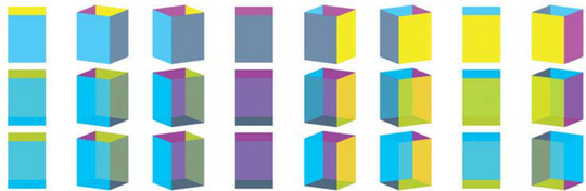
This orientation dependency is shown in Figure 11.3. A four-sided cylinder is rendered with differing orientations in three rows. The top row shows the cylinder opaque. The middle row shows a properly transparent cylinder (done with the front-and-back-facing technique described in this chapter). The bottom row shows the cylinder made transparent with no special sorting. The cylinder walls are rendered in the order magenta, yellow, gray, and cyan. As long as the walls rendered earlier are obscured by walls rendered later, the transparent cylinder is properly rendered, and the middle and bottom rows match. When the cylinder rotates to the point were the render ordering doesn’t match the depth ordering, the bottom row is incorrectly rendered. This begins happening on the fifth column, counting from left to right. Since this cylinder has only four walls, it has a range of rotations that are correct. A rounder cylinder with many facets of varying colors would be much more sensitive to orientation.
If the scene contains a single transparent object, or multiple transparent objects which do not overlap in screen space (i.e., each screen pixel is touched by at most one of the transparent objects), a shortcut may be taken under certain conditions. If the transparent objects are closed, convex, and can’t be viewed from the inside, backface culling can be used. The culling can be used to draw the back-facing polygons prior to the front-facing polygons. The constraints given previously ensure that back-facing polygons are farther from the viewer than front-facing ones.
For this, or any other face-culling technique to work, the object must be modeled such that all polygons have consistent orientation (see Section 1.3.1). Each polygon in the object should have its vertices arranged in a counter-clockwise direction when viewed from outside the object. With this orientation, the back-facing polygons are always farther from the viewer. The glFrontFace command can be used to invert the sense of front-facing for models generated with clockwise-oriented front-facing polygons.
11.9.4 Depth Peeling
An alternative to sorting is to use a multipass technique to extract the surfaces of interest. These depth-peeling techniques dissect a scene into layers with narrow depth ranges, then composite the results together. In effect, multiple passes are used to crudely sort the fragments into image layers that are subsequently composited in back-to-front order. Some of the original work on depth peeling suggested multiple depth buffers (Mammen, 1989; Diefenbach, 1996); however, in an NVIDIA technical report, Cass Everitt suggests reusing fragment programs and texture depth-testing hardware, normally used to support shadow maps, to create a mechanism for multiple depth tests, that in turn can be used to do depth peeling.
11.10 Screen-Door Transparency
Another simple transparency technique is screen-door transparency. A transparent object is created by rendering only a percentage of the object’s pixels. A bitmask is used to control which pixels in the object are rasterized. A 1 bit in the bitmask indicates that the transparent object should be rendered at that pixel; a 0 bit indicates the transparent object shouldn’t be rendered there, allowing the background pixel to show through. The percentage of bits in the bitmask which are set to 0 is equivalent to the transparency of the object (Foley et al., 1990).
This method works because the areas patterned by the screen-door algorithm are spatially integrated by the eye, making it appear as if the weighted sums of colors in Equation 11.4 are being computed, but no read-modify-write blending cycles need to occur in the framebuffer. If the viewer gets too close to the display, then the individual pixels in the pattern become visible and the effect is lost.
In OpenGL, screen-door transparency can be implemented in a number of ways; one of the simplest uses polygon stippling. The command glPolygonStipple defines a 32×32 bit stipple pattern. When stippling is enabled (using glEnable with a GL_POLYGON_STIPPLE parameter), it uses the low-order x and y bits of the screen coordinate to index into the stipple pattern for each fragment. If the corresponding bit of the stipple pattern is 0, the fragment is rejected. If the bit is 1, rasterization of the fragment continues.
Since the stipple pattern lookup takes place in screen space, the stipple patterns for overlapping objects should differ, even if the objects have the same transparency. If the same stipple pattern is used, the same pixels in the framebuffer are drawn for each object. Because of this, only the last (or the closest, if depth buffering is enabled) overlapping object will be visible. The stipple pattern should also display as fine a pattern as possible, since coarse features in the stipple pattern will become distracting artifacts.
One big advantage of screen-door transparency is that the objects do not need to be sorted. Rasterization may be faster on some systems using the screen-door technique than by using other techniques such as alpha blending. Since the screen-door technique operates on a per-fragment basis, the results will not look as smooth as alpha transparency. However, patterns that repeat on a 2×2 grid are the smoothest, and a 50% transparent “checkerboard” pattern looks quite smooth on most systems.
Screen-door transparency does have important limitations. The largest is the fact that the stipple pattern is indexed in screen space. This fixes the pattern to the screen; a moving object makes the stipple pattern appear to move across its surface, creating a “crawling” effect. Large stipple patterns will show motion artifacts. The stipple pattern also risks obscuring fine shading details on a lighted object; this can be particularly noticeable if the stippled object is rotating. If the stipple pattern is attached to the object (by using texturing and GL_REPLACE, for example), the motion artifacts are eliminated, but strobing artifacts might become noticeable as multiple transparent objects overlap.
Choosing stipple patterns for multiple transparent objects can be difficult. Not only must the stipple pattern accurately represent the transparency of the object, but it must produce the proper transparency with other stipple patterns when transparent objects overlap. Consider two 50% transparent objects that completely overlap. If the same stipple pattern is used for both objects, then the last object drawn will capture all of the pixels and the first object will disappear. The constraints in choosing patterns quickly becomes intractable as more transparent objects are added to the scene.
The coarse pixel-level granularity of the stipple patterns severely limits the effectiveness of this algorithm. It relies heavily on properties of the human eye to average out the individual pixel values. This works quite well for high-resolution output devices such as color printers (> 1000 dot-per-inch), but clearly fails on typical 100 dpi computer graphics displays. The end result is that the patterns can’t accurately reproduce the transparency levels that should appear when objects overlap and the wrong proportions of the surface colors are mixed together.
11.10.1 Multisample Transparency
OpenGL implementations supporting multisampling (OpenGL 1.3 or later, or implementations supporting ARB_multisample) can use the per-fragment sample coverage, normally used for antialiasing (see Section 10.2.3), to control object transparency as well. This method is similar to screen-door transparency described earlier, but the masking is done at each sample point within an individual fragment.
Multisample transparency has trade-offs similar to screen-door transparency. Sorting transparent objects is not required and the technique may be faster than using alpha-blended transparency. For scenes already using multisample antialiasing, a performance improvement is more likely to be significant: multisample framebuffer blending operations use all of the color samples at each pixel rather than a single pixel color, and may take longer on some implementations. Eliminating a blending step may be a significant performance gain in this case.
To implement screen-door multisample transparency, the multisample coverage mask at the start of the fragment processing pipeline must be modified (see Section 6.2) There are two ways to do this. One method uses GL_SAMPLE_ALPHA_TO_COVERAGE. When enabled, this function maps the alpha value of each fragment into a sample mask. This mask is bitwise AND’ed with the fragment’s mask. Since the mask value controls how many sample colors are combined into the final pixel color, this provides an automatic way of using alpha values to control the degree of transparency. This method is useful with objects that do not have a constant transparency value. If the transparency value is different at each vertex, for example, or the object uses a surface texture containing a transparency map, the per-fragment differences in alpha value will be transferred to the fragment’s coverage mask.
The second transparency method provides more direct control of the sample coverage mask. The glSampleCoverage command updates the GL_SAMPLE_COVERAGE_VALUE bitmask based on the floating-point coverage value passed to the command. This value is constrained to range between 0 and 1. The coverage value bitmask is bitwise AND’ed with each fragment’s coverage mask. The glSampleCoverage command provides an invert parameter which inverts the computed value of GL_SAMPLE_COVERAGE_VALUE. Using the same coverage value, and changing the invert flag makes it possible to create two transparency masks that don’t overlap. This method is most useful when the transparency is constant for a given object; the coverage value can be set once before each object is rendered. The invert option is also useful for gradually fading between two objects; it is used by some geometry level-of-detail management techniques (see Section 16.4 for details).
Multisample screen-door techniques have the advantage over per-pixel screen-door algorithms; that subpixel transparency masks generate fewer visible pixel artifacts. Since each transparency mask pattern is contained within a single pixel, there is no pixel-level pattern imposed on polygon surfaces. A lack of a visible pattern also means that moving objects won’t show a pattern crawl on their surfaces. Note that it is still possible to get subpixel masking artifacts, but they will be more subtle; they are limited to pixels that are partially covered by a transparent primitive. The behavior of these artifacts are highly implementation-dependent; the OpenGL specification imposes few restrictions on the layout of samples within a fragment.
The multisample screen-door technique is constrained by two limitations. First, it is not possible to set an exact bit pattern in the coverage mask: this prevents the application from applying precise control over the screen-door transparency patterns. While this restriction was deliberately placed in the OpenGL design to allow greater flexibility in implementing multisample, it does remove some control from the application writer. Second, the transparency resolution is limited by the number of samples available per fragment. If the implementation supports only four multisamples, for example, each fragment can represent at most five transparency levels (n + 1), including fully transparent and fully opaque. Some OpenGL implementations may try to overcome this restriction by spatially dithering the subpixel masks to create additional levels. This effectively creates a hybrid between subpixel-level and pixel-level screen-door techniques. The limited number of per-fragment samples creates a limitation which is also found in the the per-pixel screen-door technique: multisample transparency does not work well when many transparent surfaces are stacked on top of one another.
Overall, the multisample screen-door technique is a significant improvement over the pixel-level screen door, but it still suffers from problems with sample resolution. Using sorting with alpha blending can generate better results; the alpha channel can usually represent more opacity levels than sample coverage and the blending arithmetic computes an exact answer at each pixel. However, for performance-critical applications, especially when the transparent objects are difficult to sort, the multisample technique can be a good choice. Best results are obtained if there is little overlap between transparent objects and the number of different transparency levels represented is small.
Since there is a strong similarity between the principles used for modeling surface opacity and compositing, the subpixel mask operations can also be used to perform some of the compositing algorithms without using framebuffer blending. However, the limitations with respect to resolution of mask values preclude using these modified techniques for high-quality results.
11.11 Summary
In this chapter we described some of the underlying theory for image compositing and transparency modeling. We also covered some common algorithms using the OpenGL pipeline and the various advantages and limitations of these algorithms. Efficient rendering of semi-transparent objects without extra burdens on the application, such as sorting, continues to be a difficult problem and will no doubt be a continuing area of investigation. In the next chapter we examine using other parts of the pipeline for operating on images directly.