OpenGL Implementations
The OpenGL specification offers considerable flexibility to implementors. The OpenGL rendering pipeline is also an evolving design; as implementation technologies advance and new ideas surface and are proven through trial and iteration, they become part of the specification. This has both advantages and disadvantages. It ensures that the standard remains relevant for new applications by embracing new functionality required by those applications. At the same time it creates some fragmentation since different vendors may ship OpenGL implementations that correspond to different versions of the specification. This puts a greater burden on the application developer to understand the differences in functionality between the different versions and also to understand how to take advantage of the new functionality when it is available and how to do without in its absence.
In this chapter we will describe some ways in which OpenGL has evolved and is currently evolving and also discuss some interesting aspects of implementing hardware acceleration of the OpenGL pipeline.
8.1 OpenGL Versions
At the time of writing there are have been five revisions to the OpenGL specification (1.1 through 1.5). The version number is divided into a major and minor number. The change in minor number indicates that these versions are backward-compatible; no pre-existing functionality has been modified or removed. This means that applications written using an older revision of OpenGL will continue to work correctly with a newer version.
When a new version of the specification is released, it includes enhancements that either incorporate new ideas or that generalize some existing part of the pipeline. These enhancements are added as it becomes practical to implement them on existing platforms or platforms that will be available in the near future. Some examples of new functionality are the addition of vertex arrays and texture objects in OpenGL 1.1 or the addition of multitexture and multisample in OpenGL 1.3. In the case of vertex arrays and texture objects they were additions that did not really reflect new technologies. They were for the most part additions that helped improve the performance an application could achieve. Multitexture is a generalization of the texturing operation that allows multiple texture maps to be applied to a single primitive. Multisample is a new feature that introduces a new technology (multiple samples per-pixel) to achieve full-scene antialiasing.
This short list of features helps illustrate a point. Features that require new technologies or modifications to existing technologies are unlikely to be well supported on platforms that were created before the specification was defined. Therefore older platforms, i.e., older accelerators are unlikely to be refitted with new versions of OpenGL or when they do, they typically implement the new features using the host processor and are effectively unaccelerated. This means that application writers may need to be cautious when attempting to use the features from a new version of OpenGL on an older (previous generation) platform. Rather than repeat caveat emptor and your mileage may vary each time we describe an algorithm that uses a feature from a later version of OpenGL to avoid clutter we’ll only state it once here.
A fairly complete list of features added in different versions of the OpenGL specification is as follows:
OpenGL 1.1. Vertex array, polygon offset, RGB logic operation, texture image formats, texture replace environment function, texture proxies, copy texture, texture subimage, texture objects.
OpenGL 1.2. 3D textures, BGRA pixel formats, packed pixel formats, normal rescaling, separate specular color, texture coordinate edge clamping, texture LOD control, vertex array draw element range, imaging subset.
OpenGL 1.3. Compressed textures, cube map textures, multisample, multitexture, texture add environment function, texture combine environment function, texture dot3 combine environment operation, texture coordinate border clamp, transpose matrix.
OpenGL 1.4. Automatic mipmap generation, squaring blend function, constant blend color (promoted from the imaging subset), depth textures, fog coordinate, multiple draw arrays, point parameters, secondary color, stencil wrap, texture crossbar environment mode, texture LOD bias, texture coordinate mirror repeat wrap mode, window raster position.
OpenGL 1.5. Buffer objects, occlusion queries, and shadow functions.
8.2 OpenGL Extensions
To accommodate the rapid innovation in the field of computer graphics the OpenGL design also allows an implementation to support additional features. Each feature is packaged as a mini-specification that adds new commands, tokens, and state to the pipeline. These extensions serve two purposes: they allow new features to be “field tested,” and if they prove successful they are incorporated into a later version of the specification. This also allows vendors to use their innovations as product differentiators: it provides a mechanism for OpenGL implementation vendors to release new features as part of their OpenGL implementation without having to wait for the feature to become mainstream and go through a standardization process.
Over time it became useful to create standardized versions of some vendor-specific extension specifications. The original idea was to promote an existing vendor-specific extension to “EXT” status when multiple vendors (two or more) supported the extension in their implementation and agreed on the specification. It turned out that this process wasn’t quite rigorous enough, so it evolved into a new process where the Architecture Review Board creates a version of specific extensions with their own seal of approval. These “ARB” extensions often serve as previews of new features that will be added in a subsequent version of the standard. For example, multitexture was an ARB extension at the time of OpenGL 1.2 and was added to the base standard as part of OpenGL 1.3. An important purpose of an ARB extension is that it acts as a mini-standard that OpenGL implementation vendors can include in their products when they can support it well. This reduces the pressure to add new features to the base standard before they can be well supported by a broad set of implementation vendors, yet at the same time gives application writers a strong specification and an evolutionary direction.
Sometimes an ARB extension reflects a set of capabilities that are more market-specific. The ARB_imaging_subset is an example of such an extension. For this class of extensions the demand is strong enough to create a rigorously defined specification that multiple vendors can consistently implement, but the demand is not broad enough and the features are costly enough to implement so as not to incorporate it into the base standard.
As we stated in the book preface, our intent is to make full use of features available in OpenGL versions 1.0 through 1.5 as well as ARB extensions. Occasionally we will also describe a vendor-specific extension when it is helpful to a particular algorithm. More information about using extensions is included in Appendix A.
8.3 OpenGL ES for Embedded Systems
As applications for 3D graphics have arisen in areas beyond the more traditional personal computers and workstations, the success of the OpenGL standard has made it attractive for use in other areas.
One rapidly growing area is 3D graphics for embedded systems. Embedded systems range from mobile devices such as watches, personal digital assistants, and cellular handsets; consumer appliances such as game consoles, settop boxes, and printers; to more industrial aerospace, automotive, and medical imaging applications. The demands of these systems also encompass substantial diversity in terms of processing power, memory, cost, battery power, and robustness requirements. The most significant problem with the range of potential 3D clients is that many of them can’t support a full “desktop” OpenGL implementation. To solve this problem and address the needs of the embedded devices, in 2002 the Khronos Group created a group to work with Silicon Graphics (the owner of the OpenGL trademark) and the OpenGL ARB (the overseer of the OpenGL specification) to create a parallel specification for embedded devices called OpenGL ES. The operating principles of the group are to oversee a standard for embedded devices based on a subset of the existing desktop OpenGL standard. To handle the diverse requirements of all of the different types of embedded devices the Khronos Group decided to create individualized subsets that are tailored to the characteristics of a particular embedded market (Khronos Group, 2002). These subsets are termed profiles.
8.3.1 Embedded Profiles
To date, the Khronos Group has completed version 1.0 and 1.1 of the specifications for two profiles (Blythe, 2003) and is in the process of creating the specification for a third. Profile specifications are created by working groups, comprised of Khronos members experienced in creating OpenGL implementations and familiar with the profile’s target market. Since a profile is intended to address a specific market, the definition of a profile begins with a characterization of the market being addressed, analyzing the demands and constraints of that market. The characterization is followed by draft proposals of features from the desktop OpenGL specification that match the market characterization document. From the feature proposals a more detailed specification document is created. It defines the exact subset of the OpenGL pipeline included in the profile, detailing the commands, enumerants, and pipeline behavior. Similar to OpenGL ARB extensions, an OpenGL ES profile specification may include new OES extensions that are standardized versions of extensions useful to the particular embedded market. Like desktop OpenGL implementations, implementations of OpenGL ES profiles may also include vendor-specific extensions. The set of extensions include those already defined for desktop OpenGL, as well as new extensions created specifically to address additional market-specific needs of the profile’s target market.
A profile includes a strict subset of the desktop OpenGL specification as its base and then adds additional extensions as either required or optional extensions. Required extensions must be supported by an implementation and optional extensions are at the discretion of the implementation vendor. Similar to desktop OpenGL, OpenGL ES profiles must pass a profile-specific conformance test to be described as an OpenGL ES implementation. The conformance test is also defined and overseen by the Khronos Group.
The two defined profiles are the Common and Common-Lite profiles. The third profile design in progress is the Safety Critical profile.
8.3.2 Common and Common-Lite Profiles
The goal of the Common and Common-Lite profiles is to address a wide range of consumer-related devices ranging from battery-powered hand-held devices such as mobile phones and PDAs to line-powered devices such as kiosks and settop boxes. The requirements of these devices are small memory footprint, modest to medium processing power, and a need for a wide range of 3D rendering features including lighted, texture mapped, alpha blended, depth-buffered triangles, lines, and points.
To span this broad range of devices, there are two versions of the profile. The Common profile effectively defines the feature subset of desktop OpenGL in the two profiles. The Common-Lite profile further reduces the memory footprint and processing requirements by eliminating the floating-point data type from the profile.
The version 1.0 Common profile subset is as follows: Only RGBA rendering is supported, color index mode is eliminated. The double-precision data type is dropped and a new fixed-point data type called fixed (suffixed with ‘x’) is added. Desktop OpenGL commands that only have a double-precision form, such as glDepthRange are replaced with single-precision floating-point and fixed-point versions.
Only triangle, line, and point-based primitives are supported (not pixel images or bitmaps). Geometry is drawn exclusively using vertex arrays (no support for glBegin/glEnd). Vertex arrays are extended to include the byte data type.
The full transformation stack is retained, but the modelview stack minimum is reduced to 16 elements, and the transpose forms of the load and multiply commands are removed. Application-specified clipping planes and texture coordinate generation are also eliminated. Vertex lighting is retained with the exception of secondary color, local viewer mode, and distinct front and back materials (only the combined GL_FRONT_AND_BACK material can be specified). The only glColorMaterial mode supported is the default GL_AMBIENT_AND_DIFFUSE.
Rasterization of triangles, lines, and points are retained including flat and smooth shading and face culling. However, polygon stipple, line stipple, and polygon mode (point and line drawing styles) are not included. Antialiased line and point drawing is included using glLineSmooth and glPointSmooth, but not glPolygonSmooth. Full scene antialiasing is supported through multisampling, though it is an optional feature.
The most commonly used features of texture mapping are included. Only 2D texture maps without borders using either repeat or edge clamp wrap modes are supported. Images are loaded using glTexImage2D or glCopyTexture2D but the number of external image type and format combinations is greatly reduced. Table 8.1 lists the supported combinations of formats and types. The infrastructure for compressed texture images is also supported. The Common and Common-Lite profiles also introduce a simple paletted form of compression. The extension is defined so that images can either be accelerated in their indexed form or expanded to their non-paletted form at load time operating on them as regular images thereafter.
Table 8.1
OpenGL ES Texture Image Formats and Types
| Internal Format | External Format | Type |
| GL_RGBA | GL_RGBA | GL_UNSIGNED_BYTE |
| GL_RGB | GL_RGB | GL_UNSIGNED_BYTE |
| GL_RGBA | GL_RGBA | GL_UNSIGNED_SHORT_4_4_4_4 |
| GL_RGBA | GL_RGBA | GL_UNSIGNED_SHORT_5_5_5_1 |
| GL_RGB | GL_RGB | GL_UNSIGNED_SHORT_5_6_5 |
| GL_LUMINANCE_ALPHA | GL_LUMINANCE_ALPHA | GL_UNSIGNED_BYTE |
| GL_LUMINANCE | GL_LUMINANCE | GL_UNSIGNED_BYTE |
| GL_ALPHA | GL_ALPHA | GL_UNSIGNED_BYTE |
Multitexturing is supported, but only a single texture unit is required. Texture objects are supported, but the set of texture parameters is reduced, leaving out support for texture priorities and level clamping. A subset of texture environments from the OpenGL 1.3 version are supported: GL_MODULATE, GL_BLEND, GL_REPLACE, GL_DECAL, and GL_ADD. The remainder of the pipeline: fog, scissor test, alpha test, stencil/depth test, blend, dither, and logic op are supported in their entirety. The accumulation buffer is not supported.
Support for operating on images directly is limited. Images can be loaded into texture maps, and images can be retrieved to the host from the framebuffer or copied into a texture map. The glDrawPixels, glCopyPixels, and glBitmap commands are not supported.
More specialized functionality including evaluators, feedback, and selection are not included. Display lists are also omitted because of their sizable implementation burden. State queries are also substantially limited; only static state can be queried. Static state is defined as implementation-specific constants such as the depth of a matrix stack, or depth of color buffer components, but does not include state that can be directly or indirectly set by the application. Examples of non-static state include the current blend function, and the current value of the modelview matrix.
Fixed-Point Arithmetic
One of the more significant departures from desktop OpenGL in the Common profile is the introduction of a fixed-point data type. The definition of this type is a 32-bit representation with a 16-bit signed integer part and a 16-bit fraction part. Conversions between a fixed-point representation, x, and a traditional integer or floating-point representation, t, are accomplished with the formulas:
which, of course, may use integer shift instructions in some cases to improve the efficiency of the computation. The arithmetic rules for fixed-point numbers are:
Note that the simple implementation of multiplication and division need to compute a 48-bit intermediate result to avoid losing information.
The motivation for adding the fixed-point data type is to support a variety of devices that do not include native hardware support for floating-point arithmetic. Given this limitation in the devices, the standard could either:
1. Continue to support single-precision floating-point only, assuming that software emulation will be used for all floating-point operations (in the application and in the profile implementation).
2. Require a floating-point interface but allow the profile implementation to use fixed-point internally by relaxing some of the precision and dynamic range requirements. This assumes that an application will use software floating-point, or will use its own form of fixed-point within the application, and convert to floating-point representation when using profile commands.
3. Support a fixed-point interface and internal implementation including relaxing the precision and dynamic range requirements.
Each of the choices has advantages and disadvantages, but the path chosen was to include a fixed-point interface in both the Common and Common-Lite profiles, while requiring the Common profile to continue to support a dynamic range consistent with IEEE single-precision floating-point. This allows an application to make effective use of either the floating-point data types and command interface while retaining compatibility with Common-Lite profile applications. The Common-Lite profile only supports fixed-point and integer data types and at minimum must support a dynamic range consistent with a straightforward fixed-point implementation with 16 bits each of integer and fraction parts. However, a Common-Lite profile implementation may support larger dynamic range, for example, using floating-point representations and operations internally.
This design decision places more burden on applications written using the fixed-point interface to constrain the ranges of values used within the application, but provides opportunities for efficient implementations across a much wider range of device capabilities.
The principal application concern is avoiding overflow during intermediate calculations. This means that the combined magnitudes of values used to represent vertices and modeling transformations must not exceed 215 − 1. Conversely, given the nature of fixed-point arithmetic, values less than 1.0 will lose precision rapidly. Some useful rules for avoiding overflow are:
Given a representation that supports numbers in the range [−X, X],
1. Data should start out within this range.
2. Differences between vertex components within a primitive (triangle or line) should be within [−X, X].
3. For any pair of vertices q and p, |qi−pi| + |q3−p3| <X, for i = 0 … 2 (the subscript indices indicate the x, y, z, and w components).
These constraints need to be true for coordinates all the way through the transformation pipeline up to clipping. To check that this constraint is met for each object, examine the composite transformation matrix (projection*modelview) and the components of the object vertices. Take the absolute values of the largest scaling component from the upper 3 × 3 (s), the largest translational component from the 4th column (t), and the largest component from the object vertices (c), and test that c * s + t < X/2.
8.3.3 Safety Critical Profile
The Safety Critical profile addresses the market for highly robust or mission critical 3D graphics implementations. Typical applications for this market include avionics and automotive displays. The principal driving factor behind the Safety Critical profile is providing the minimum required 3D rendering functionality and nothing more. Unlike the Common profile, processing power, battery power, and memory footprint are not constraints. Instead, minimizing the number of code paths that need to be tested is much more important. For these reasons, the Safety Critical profile greatly reduces the number of supported input data types, and will make more drastic cuts to existing desktop features to simplify the testing burden.
8.3.4 OpenGL ES Revisions
The OpenGL ES embedded profiles promise to extend the presence of the OpenGL pipeline and OpenGL applications from tens of millions of desktop computers to hundreds of millions of special purpose devices. Similar to the OpenGL specification, the ES profile specifications are also revised at regular intervals, nominally yearly, so that important new features can be incorporated into the standard in a timely fashion.
8.4 OpenGL Pipeline Evolution
Looking at features added to new versions, the most significant changes in OpenGL have occurred in the way data is managed and moved in and out of the pipeline (texture objects, vertex arrays, vertex buffer objects, render-to-texture, pbuffers, packed pixels, internal formats, subimages, etc.) and in the explosive improvement in the capabilities of the texture mapping subsystem (cube maps, LOD control, multitexture, depth textures, combine texture environment, crossbar environment, etc.). The first class of changes reflect a better understanding of how applications manage data and an evolving strategy to tune the data transfer model to the underlying hardware technologies. The second class of changes reflect the desire for more advanced fragment shading capabilities.
However, these changes between versions only tell part of the story. The OpenGL extensions serve as a harbinger of things to come. The most significant feature is the evolution from a fixed-function pipeline to a programmable pipeline. This evolution manifests itself in two ways: vertex programs and fragment programs. Vertex programs allow an application to tailor its own transform and lighting pipeline, enabling more sophisticated modeling and lighting operations including morphing and skinning, alternate per-vertex lighting models, and so on. Fragment programs bypass the increasingly complex multitexture pipeline API (combine and crossbar environments), replacing it with a complex but much more expressive programming model allowing nearly arbitrary computation and texture lookup to be performed at each fragment.
The two programmable stages of the pipeline continue to grow in sophistication, supporting more input and computational resources. However, there is another evolutionary stage just now appearing. The programmable parts of the pipeline are following the evolution of traditional computing (to some extent), beginning with programs expressed in a low-level assembly language and progressing through languages with increased expressiveness at a much higher level. These improvements are achieved through the greater use of abstraction in the language. The programmable pipeline is currently making the first transition from assembly language to a higher-level (C-like) language. This step is embodied in the ARB_shading_language_100 extension, also called the OpenGL Shading Language (Kessenich et al., 2003).
The transition to a higher-level shading language is unlikely to be the end of the evolution, but it may signal a marked slow down in the evolution of the structure of the pipeline and greater focus on supporting higher-level programming constructs. Regardless, the transition for devices to the programmable model will take some time, and in the near term there will be devices that, for cost or other reasons, will be limited to earlier versions of the OpenGL standard well after the programmable pipeline becomes part of core OpenGL.1
The remainder of this chapter describes some of the details and technologies involved in implementing hardware accelerators. Many of the techniques serve as a basis for hardware-accelerated OpenGL implementations independent of the target cost of the accelerator. Many of the techniques can be scaled down for low-cost or scaled up for very high-performance implementations and the techniques are applicable to both the fixed-function and programmable parts of the pipeline.
8.5 Hardware Implementations of the Pipeline
The speed of modern processors makes it possible to implement the entire OpenGL pipeline in software on the host processor and achieve the performance required to process millions of vertices per second and hundreds of millions of pixels per second. However, the trend to increase realism by increasing the complexity of rendered scenes calls for the use of hardware acceleration on at least some parts of the OpenGL pipeline to achieve interactive performance.
At the time of this writing, hardware acceleration can enable performance levels in the range of 100 to 300 million vertices per second for geometry processing and 100 million to 5 billion pixels per second for rasterization. The raw performance is typically proportional to the amount of hardware acceleration present and this is in turn reflected in the cost and feature set of the accelerator. OpenGL pipelines are being implemented across a tremendous range of hardware and software. This range makes it difficult to describe implementation techniques that are applicable across devices with differing price and performance targets. Instead, the following sections provide an overview of some acceleration techniques in order to provide additional insight into how the pipeline works and how applications can use it more efficiently.
The OpenGL pipeline can be roughly broken into three stages: transform and lighting, primitive setup, and rasterization and fragment processing. Accelerators are usually designed to accelerate one or more of these parts of the pipeline. Usually there is more benefit in accelerating the later stages of the pipeline since there is more data to process.
8.5.1 Rasterization Acceleration
Rasterization accelerators take transformed and lighted primitives and convert them to pixels writing them to the framebuffer. The rasterization pipeline can be broken down into several operations which are described in the following paragraphs.
Scan Conversion
Scan conversion generates the set of fragments corresponding to each primitive. Each fragment contains window coordinates x, y, and z, a color value, and texture coordinates. The fragment values are generated by interpolating the attributes provided at each vertex in the primitive. Scan conversion is computationally intensive since multiple attribute values must be computed for each fragment. Scan conversion computations can be performed using fixed-point arithmetic, but several of the computations must be performed at high precision to avoid producing artifacts. For example, color computations may use 4- or 8-bit (or more) computations and produce satisfactory results, whereas window coordinates and texture coordinates need substantially higher precision. During scan conversion the generated fragments are also tested against the scissor rectangle, and fragments outside the rectangle are discarded.
Texture
Texture mapping uses texture coordinates to look up one or more texel values in a texture map. The texel values are combined together to produce a single color, which is used to update the fragment color. The update method is determined by the current texture environment mode. The texturing operation can be both computationally expensive and memory intensive, depending on the filtering mode. For example, an RGBA texture map using a GL_LINEAR_MIPMAP_LINEAR minification filter retrieves 8 texel values split between 2 texture images. These 8 texel values are combined together using roughly 10 multiplications and 4 additions per color component. The amount of memory bandwidth required is dependent on the component number and depth of the texture map as well as the type of filtering used. It is common for hardware accelerators to design around compact texel representations, for example, 16-bit texels (textures with component sizes summing to 16-bits or less such as GL_RGBA4, GL_RGB5_A1) or a compressed texture representation.
Multitexture increases the bandwidth requirement in a linear way, in that each active texture stage requires a similar set of operations to produce the filtered result and then the result must be combined with those from other texture stages.
Fog and Alpha
This stage calculates an attenuation value, used to blend the fragment color with a fog color. The attenuation computation is dependent on the distance between the eye and the fragment and the current fog mode. Many hardware accelerators use the window z coordinate as an approximation to the distance, evaluating the fog function using a table lookup scheme rather than providing circuitry to evaluate the fog function directly.
The alpha function compares the fragment alpha against a reference value and performs an interpolation between the alpha and selected color components of the fragment. The color components selected depend on the current alpha function.
Depth and Stencil
The depth and stencil tests are memory intensive, since the depth and stencil values must be retrieved from the framebuffer before the tests can be performed. The amount of memory bandwidth required depends on the size of the depth and stencil buffers. Accelerator implementations will often pack the depth and stencil storage together for simultaneous access. For example, a 23-bit depth value and 1-bit stencil value are packed into 3 bytes, or a 24-bit depth value and an 8-bit stencil value are packed into 4 bytes. In the first example, the stencil operation may be no more expensive than the depth test operation if memory is accessed in byte-units; but in the latter case the stencil operation may cost an extra memory access, depending on the structure of the memory interface.
Blending
Framebuffer blending is also memory intensive since the contents of the color buffer must be retrieved as part of the computation. If the blend function uses destination alpha, additional memory bandwidth is required to retrieve the destination alpha value. Depending on the blend function, a moderate number of multiplication and addition operations may also be required. For example, for rendering of transparent surfaces, 6 multiplies and 3 adds are required for each fragment:
Framebuffer Operations
Rasterization accelerators typically accelerate some additional framebuffer operations such as buffer clears and dithering. The clear operations are very memory intensive, since every pixel within the window needs to be written. For example, a 1024×1024 window requires 1 million memory operations to write each pixel in the window. If an application is running at 85 frames per second, 85 million pixel writes per second are required just to clear the window.
Accumulation buffer operations are also computation and memory intensive, but frequently are not implemented directly in lower cost accelerators. The main reason for this is that the accumulation buffer operations require larger multipliers and adders to implement the higher precision arithmetic, but the cost is prohibitive for lower cost accelerators.
The total number of rasterization computations performed for each pixel can exceed 100 operations. To support rasterization rates in excess of 100 million pixels per second the rasterization pipeline must support as many as 1 billion operations per second or more. This is why rasterization acceleration is found in all but the lowest-cost devices that support 3D rendering.
OpenGL implementations that do not use an external accelerator may still take advantage of special CPU instructions to assist with rasterization. For example, Intel’s MMX (multimedia extensions) (Peleg et al., 1997) instructions allow the same operation to be simultaneously applied to multiple data elements packed into a wide register. Such instructions are particularly useful for computing all of the components of an RGBA color value at once.
8.5.2 Primitive Setup Acceleration
Primitive setup refers to the set of computations that are required to generate input fragments for the rasterization pipeline. In lowest cost accelerators, these computations are performed on the host computer for each primitive and sent to the rasterizer. These computations can easily become the bottleneck in the system, however, when a large number of primitives are drawn. The computations require computing the edge equations for each active parameter in a triangle’s vertices (color, depth, texture coordinates), performed at high precision to avoid artifacts. There is a large amplification of the amount of data in the pipeline, as each triangle generates a large number of fragments from three vertices.
8.5.3 Transform and Lighting Acceleration
Mid-range and high-end accelerators often provide hardware acceleration for the OpenGL transform and lighting (also called geometry) operations. These operations include the transformation of vertex coordinates to eye space, lighting computations, projection to window coordinates, clipping, texture coordinate generation, and transform. These operations typically use IEEE-754 single-precision floating-point computations2 and require in excess of 90 operations per-vertex when lighting or texturing is enabled. To achieve rates of 10 million triangles per second, more than 100 million floating-point operations per second are necessary in addition to data movement and other operations. High vertex rates preclude using the host CPU except in cost-sensitive applications.
Even with accelerator support, some operations need to be implemented carefully to achieve good performance. For many computations, it is not necessary to evaluate the result to full single-precision accuracy. For example, color computations may only need 8- or 12-bits of precision, and specular power and spotlight power functions are often implemented using table lookup rather than direct function evaluation. The OpenGL glRotate command may use limited precision polynomial approximations to evaluate trigonometric functions. Division may be implemented using fast reciprocal approximations (Soderquist and Leeser, 1996) rather than a much more expensive divide operation. The accelerator architecture may be tuned to compute inner product operations since much of the transformation and lighting computations are composed of inner product computations.
Implementations that support programmable vertex operations (vertex programs), map or translate the application-specified vertex programs onto an internal instruction set. This internal instruction set shares much in common with the operations required to implement the fixed vertex pipeline: vector add, multiply, reciprocal, inner product, matrix operations, limited conditional branching and looping, and miscellaneous operations to assist in computing some parts of the vertex lighting equation (e.g., attenuation or specular power). Programmable fragment processing requires similar types of instructions as well, particularly to support per-fragment lighting computations, only in the near-term with lower precision and range requirements than those needed for vertex processing.
Over the past five years, it has become cost-effective to fit rasterization, setup, and transform and lighting acceleration into a single chip, paving the way for low-cost implementations to hardware accelerate the majority of the OpenGL pipeline. These implementations range from desktop to handheld devices. High-end desktop versions are capable of rendering hundreds of millions of triangles per second and billions of pixels per second, while low-power consumption, low-cost implementations for hand-held devices are capable of hundreds of thousands of triangles and tens of millions of pixels per second.3
8.5.4 Pipeline Balance
The data explosion that occurs as vertices are processed and converted to pixels leads to the notion of balancing the stages of the pipeline to match the increases in the amount of data to be processed. An unbalanced pipeline leaves a bottleneck at one of the pipeline stages, leaving earlier and later stages idle, wasting resources. The question arises on how to determine the correct balance between pipeline stages. The difficulty is that the correct answer is application-dependent. An application that generates large numbers of very small triangles may require more power in the earlier transform, lighting, and setup stages of the pipeline, whereas applications that generate smaller numbers of triangles with larger areas may require more rasterization and pixel fill capabilities. Sometimes application classes can be grouped into categories such as geometry-limited or fill-limited. Generally CAD applications fit in the former category, whereas games and visual simulation applications fit in the latter, so it is not uncommon for accelerator designers to bias their implementations toward their target audience.
One way to describe the balance is in terms of the number of input triangles (or other primitives) and the average area of the primitive. For example, 100 million triangles per second with 10 pixels per triangle requires 1 billion pixels to be processed per second. Similarly, 50 million 10-pixel aliased lines may require 500 million pixels per second, and 50 million antialiased lines where each antialiased pixel has a 3-pixel footprint requires 1.5 billion pixels per second. System designers will then assign properties to the primitives and pixels, (e.g., a single infinite light; normal, color, one texture coordinate per-vertex; average triangle strip length 10; 2 mipmapped textures; depth buffering; 8-bit RGBA framebuffer; 24-bit depth buffer, etc.) and determine the raw processing requirements to meet these objectives.
8.5.5 Parallelism Opportunities
The OpenGL specification allows the use of parallel processing to improve performance, but imposes constraints on its use. The most important constraint requires that images are rendered as if their primitives were processed in the order they were received, throughout the pipeline. This means that the fragments from one triangle shall not reach the framebuffer before the fragments of a triangle that was sent to the pipeline earlier. This constraint is essential for the correct operation of order-dependent algorithms such as transparency. However, the specification does not prohibit primitives from being processed out of order, as long as the end result isn’t changed.
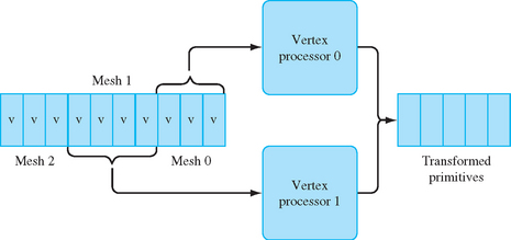
Parallelism can be exploited in the transform and lighting stages by processing vertices in parallel, that is, by processing two or more vertices simultaneously. Much of the vertex processing can be performed completely in parallel (transforms, lighting, clip testing) and the results accumulated for primitive assembly and rasterization. A parallel implementation can take several forms. Individual primitives can be sent to independent processors for processing, and the resultant primitives merged back in order before rasterization, as shown in Figure 8.1. In such an implementation, the incoming primitives are passed through a distributor that determines to which geometry processor to send each primitive. The distributor may choose processors in a round-robin fashion or implement a more sophisticated load-balancing scheme to ensure that primitives are sent to idle processors. The output of each geometry processor is sent to a recombiner that merges the processed primitives in the order they were originally sent. This can be accomplished by tagging the primitives in the distributor and then reassembling them in the order specified by the tags.
Using multiple-instruction-multiple-data (MIMD) processors, the processors can run independently of one another. This allows different processors to process differing primitive types or lengths or even execute different processing paths, such as clipping a primitive, in parallel. MIMD-based processing can support workloads with greater variation, but incurs the extra cost of supporting a complete processor with instruction sequencing and data processing. An alternative is to run the processors in lockstep using a single instruction stream.
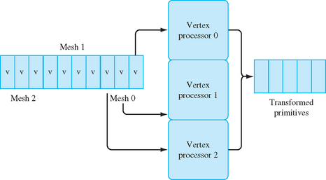
A single-instruction-multiple-data (SIMD) processor can be used to process the vertices for a single primitive in parallel. For example, a SIMD processor with three processors can simultaneously process the three vertices in an independent triangle, or three vertices at a time from a triangle strip, as shown in Figure 8.2. Clipping computations are more difficult to process in parallel on an SIMD processor, so most SIMD implementations use a single processor to clip a primitive.
In both these cases, difficulties arise from state changes, such as changing the modelview matrix or the current color. These changes must be applied to the correct set of primitives. One reason that OpenGL allows so few commands between glBegin/glEnd sequences is to facilitate parallel processing without interference from state changes.
When there are no state changes between primitives, all of the vertices for the set of primitives can be processed in the same way. This allows the simple SIMD model to be extended to process vertices from multiple primitives at once, increasing the width of the SIMD array. As the vertices are being processed, the information defining which vertices are contained within each input primitive must be preserved and the primitives re-assembled before clipping.
A single large SIMD array may not be effectively utilized if there are frequent state changes between primitives, since that reduces the number of vertices that are processed identically. One method to maintain efficiency is to utilize an MIMD array of smaller SIMD processors where each MIMD element processes vertices with a particular set of state. Multiple MIMD elements can work independently on different primitives, while within each MIMD element, a SIMD array processes multiple vertices in parallel.
Vertex Efficiency
Most hardware accelerators are tuned to process connected primitives with no interleaved state changes with maximum efficiency. Connected primitives, such as triangle strips, allow the cost of processing a vertex to be amortized over multiple primitives. By avoiding state changes, the geometry accelerator is free to perform long sequences of regular vector and matrix computations and make very efficient use of the arithmetic logic in the accelerator. This an area where the use of vertex arrays can improve performance, since state changes cannot be interspersed in the vertex data and the vertex array semantics leave the current color, normal, and texture coordinate state undefined at the end of the array.
Vertex Caching
Implicitly connected primitives such as strips and fans are not the only mechanism for amortizing vertex computations. Vertex arrays can also be used to draw triangle lists, that is, indexed arrays of triangles using the glDrawElements command. At first glance, indexed arrays may seem inefficient since an index must first be fetched before the vertex data can be fetched. However, if the index values are compact (16-bits) and can be fetched efficiently by the accelerator, indexing allows more complex topologies than strips and fans to be specified in a single rendering command. This allows meshes to be specified in which more than two primitives can share each vertex. For example, a regular rectangular grid of triangles will reuse each vertex in four triangles in the interior. This means that the cost of fetching index values can be overcome by the savings from avoiding re-transforming vertices. To realize the savings the accelerator needs to be able to track the post-transform vertex data and re-use it.
With connected primitives the vertex data is re-used immediately as part of the next primitive. However, with mesh data each triangle must be specified completely, so some vertices must be re-specified. Fortunately, vertices are uniquely indexed by their index value, so the index value can also be used to index a post-transform vertex cache to retrieve already transformed values. This cache can be implemented as a software-managed cache (for example, in implementations that do software vertex processing), or it can be implemented directly in hardware. A relatively small cache of 8 to 16 entries, combined with careful ordering of the individual primitives in the triangle list, can result in very good vertex re-use, so this technique is commonly employed.
Rasterization
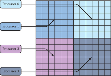
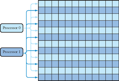
Parallelism can be exploited in the rasterization stage during fragment processing. Once a fragment is generated during scan conversion, it can be processed independently of other fragments as long as order is preserved. One way to accomplish this is to subdivide the screen into regions and assign fragment processors to different regions as shown in Figure 8.3. After scan conversion, each fragment is assigned to a processor according to its window coordinates. A coarse screen subdivision may result in poor processor utilization if the polygons are not evenly distributed among the subdivided regions. To achieve better load balancing, the screen may be more finely subdivided and multiple regions assigned to a single fragment processor. Scan-line interleave is one such form of fine-grain subdivision: each region is a scan line, and multiple scan lines are assigned to a single processor using an interleaving scheme, as shown in Figure 8.4
Similar SIMD processing techniques can also be used for fragment processing. Since all of the pixels of a primitive are subject to the identical processing, they can be processed in parallel.
One place where parallelism is particularly effective is in improving memory access rates. Two places where external memories are heavily accessed are texture lookup and framebuffer accesses. Rasterization bottlenecks often occur at the memory interfaces. If external memory can’t keep up with the rest of the rasterizer, the pixel rate will be limited by the rate at which memory can be accessed; that is, by the memory bandwidth. Parallelism increases the effective memory bandwidth, by spreading the burden of memory accesses over multiple memory interfaces. Since pixels can be processed independently, it is straightforward to allocate memory interfaces to different pixel regions using the tiling technique described previously.
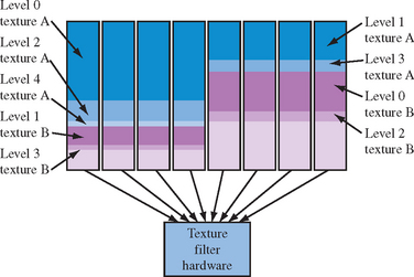
For texture memory accesses, there are several ways of achieving some parallelism. For mipmapping operations using GL_LINEAR_MIPMAP_LINEAR filtering, eight texel values are retrieved from two mipmap levels. Rather than fetch the texel values serially, waiting for each access to complete before starting the next one, the mipmap levels can be distributed between multiple memories using a tiling pattern. Interleaving data across multiple memory interfaces can benefit any texture filter that uses more than one sample. In addition to interleaving, entire levels can also be replicated in independent memories, trading space for improved time by allowing parallel conflict-free access. Figure 8.5 illustrates an example where texture memory is replicated four ways and even and odd mipmap levels are interleaved.
An alternative to multiple external texture memories is to use a hierarchical memory system. This system has a single external interface, combined with an internal cache memory, which allows either faster or parallel access. Hierarchical memory schemes rely on coherency in the memory access pattern in order to re-use previous memory fetches. Fortunately, mipmapping can exhibit a high level of coherency making caching effective. The coherency can be further improved using texture compression to reduce the effective memory footprint for a texture at the cost of additional hardware to decompress the texture samples during lookup. The organization of memory affects the performance of the texturing subsystem in significant way; in older accelerators it was common for mipmapping to be slower than linear or other filters in the absence of replication and interleaving. In modern low-cost accelerators it is common for applications using mipmap filters to achieve better performance than linear filters since small mipmap levels have better cache coherency than larger linear maps.
A second way to increase parallelism can be exploited for multitexturing operations. If multiple textures are active and the texture coordinates are independent of one another, then the texel values can be retrieved in parallel. Again, rather than multiple external memories, a single external memory can be used with a parallel or high-speed internal cache. Like modern processor memory systems, the caching system used for texturing can have multiple levels creating a hierarchy. This is particularly useful for supporting the multiple texture image references generated by multitexturing and mipmapping.
Latency Hiding
One of the problems with using memory caching is that that the completion times for memory reads become irregular and unpredictable. This makes it much more difficult to interleave memory accesses and computations in such a way as to minimize the time spent idle waiting for memory reads to complete. There can be substantial inefficiency in any processing scheme if the processing element spends a lot of time idle while waiting for memory references to complete. One way to improve efficiency is to use a technique called hyperthreading. In hyperthreading, instead of having the processing element sit idle, the processor state is saved and the processor executes another waiting task, called a thread. If the second thread isn’t referencing memory and executes some amount of computation, it can overlap the waiting time or latency, of the memory reference from the first thread. When the memory reference for the first thread completes, that thread is marked as “ready” and executes the next time the processing element stalls waiting for a memory reference. The cost of using the hyperthreading technique is that extra hardware resources are required to store the thread state and some extra work to stop and start a thread.
Hyperthreading works well with highly parallel tasks such as fragment processing. As fragments are generated during rasterization, new threads corresponding to fragments are constructed and are scheduled to run on the processing elements. Hyperthreading can be mixed with SIMD processing, since a group of fragments equal to the SIMD array width can be treated as a single thread. SIMD processing has the nice property that its lockstep execution means that all fragments require memory reads at the same instant. This means that its thread can be suspended once while its read requests for all of the fragments are serviced.
Early-Z Processing
Another method for improving rasterization and fragment processing performance is to try to eliminate fragments that are not visible before they undergo expensive shading operations. One way to accomplish this is to perform the depth test as fragments are generated. If the fragment is already occluded then it is discarded immediately avoiding texture mapping and other operations. To produce correct images, the early test must produce identical results compared to depth testing at the end of the pipeline. This means that when depth testing is disabled, or the depth function is modified, the early depth test must behave correctly.
While early testing against the depth buffer can provide a useful optimization, it still requires comparing each fragment against the corresponding depth buffer location. In implementations with deep buffers of fragments traveling through the fragment processing path on the way to the framebuffer, the test may be using stale depth data. An alternative is to try to reject more fragments from a primitive in a single test, by using a coarser depth buffer consisting of a single value for a tile or super-pixel. The coarser buffer need only store information indicating whether the super-pixel is completely occluded and if so, its min and max depth values in the area covered. Correspondingly large areas from an incoming primitive are tested against the depth range stored in the super-pixel. The results of the test: completely behind the super-pixel, completely in front of the super-pixel, or intersects determine if the incoming block of pixels is discarded, or processed as normal (with the depth range in the super-pixel updated as necessary).
Special cases arise when the incoming area intersects the depth range of the super-pixel, or the incoming area is completely in front, but doesn’t completely cover the super-pixel. In both cases the fragments in the incoming area proceeds through the rest of the pipeline, but the super-pixel is invalidated since it isn’t completely covered by the incoming primitive.
Despite the additional complexity of the coarser area approximation, it has two advantages. First, it can reject larger groups of incoming fragments with few tests. Second, if the areas are large enough (16×16), the buffer storing the depth range and valid flag for the super-pixel becomes small enough to fit on-chip in a hardware accelerator, avoiding additional delays retrieving values from memory. To further improve the efficiency of rejection, the scheme can be extended to a hierarchy of tile sizes (Greene et al., 1993).
8.5.6 Reordering the Pipeline
The early-Z processing mechanism is one of a number of places where processing steps can be reordered to eliminate unnecessary work as a form of performance optimization. The idea is to move work earlier in the pipeline to eliminate other potentially unnecessary processing later in the pipeline. Some examples of this are trivial rejection of primitives and backface culling. The logical order for processing primitives is to transform them to eye-space; light them; project to clip space; clip or discard primitives outside the view volume; perform the perspective division and viewport transformation. However, it can be more efficient to defer the vertex lighting computation until after the trivial rejection test, to avoid lighting vertices that will be discarded. Similarly, polygon face culling logically happens as part of polygon rasterization, but it can be a significant performance improvement to cull polygons first, before lighting them.
In the rasterization and fragment processing stages, it is similarly common to perform the scissor test during rasterization. This ensures that fragments are discarded before texture mapping or expensive shading operations. Early-Z and stencil processing are perhaps the most complex examples, since all application-visible side effects must be maintained. This is the key constraint with reordering the pipeline; it must be done in such a way that the application is unaware of the ordering change; all side effects must be preserved. Side effects might include updates to ancillary buffers, correct output of feedback and selection tokens, and so forth.
The idea of eliminating work as early as possible isn’t limited to the internal implementation of the pipeline. It is also beneficial for applications to try to take similar steps, for example, using alpha testing with framebuffer blending to discard “empty” fragments before they reach the more expensive blending stage of the pipeline. Chapter 21 discusses these additional performance optimization techniques.
8.5.7 Mixed Software and Hardware Implementations
As OpenGL continues to evolve, and this single standard is used to satisfy a wide range of applications over an even larger range of performance levels, it is rare for implementations to hardware accelerate all OpenGL primitives for every possible combination of OpenGL states.
Instead, most implementations have a mixture of hardware accelerated and unaccelerated paths. The OpenGL specification describes pipelines of steps that primitives must go through to be rendered. These pipelines may be implemented in software or accelerated in hardware. One can think of an implementation containing multiple pipelines, each associated with a set of OpenGL state settings, called a state vector. Each one of these pipeline/state combinations is a path.
A hardware designer may choose to hardware accelerate only a subset of all possible OpenGL states to reduce hardware costs. If an application sets a combination of state settings that aren’t accelerated, primitives processed under that state will be rendered using software on the host processor. This concept gives rise to a number of notions, including fast paths, slow paths, and fall back to software, to indicate whether an implementation is or is not using a high-performance path for a particular combination of modes.
The existence of software and hardware paths has obvious performance implications, but it also introduces some subtler issues. In Section 6.1.1 the importance of invariance in rasterization for multipass algorithms was emphasized. As a practical matter, however, it can be very difficult for an implementation with mixed software and hardware paths to guarantee consistency between them. For example, if a new blending mode is introduced, a software rasterization path may be added to the implementation to support the new mode on legacy hardware. It may be difficult to use this mode in a multipass algorithm since the software rasterizer is unlikely to rasterize triangles in the same way as the hardware.
It may not be an entire path that is implemented in software, but just a single operation. For example, accumulation buffer operations are commonly performed on the host processor, as the extended precision arithmetic is too expensive to implement in commodity hardware. Another example is texture borders. Texture borders, by their nature, tend to complicate hardware texturing implementations and they are not used by many applications;4 as a result, they are often relegated to software paths, or occasionally not supported at all.
8.6 The Future
It’s difficult to predict exactly how the OpenGL pipeline will continue to evolve, but some directions seem promising. In particular, the enhancement of the programmable parts of the pipeline (vertex and fragment programs) will continue, adding storage and computational resources, as well as enhanced arithmetic. Concurrently, new processing structuring paradigms such as stream processing (Owens et al., 2000) may help scale hardware accelerators to the next order of magnitude in performance improvement. At the same time, interest continues in adding new functionality to the pipeline, such as support for subdivision surfaces and displacement mapping (Lee et al., 2000). The demand for efficient implementations of such features may see the evolution of the traditional polygon-based OpenGL rendering pipeline to other form ulations such as REYES (render everything you ever saw) (Cook et al., 1987; Owens et al., 2002) allowing hardware accelerators to achieve the next level of interactive realism. In the meantime, the software and hardware implementation techniques described here will enjoy continued use across a variety of devices for the foreseeable future.
1OpenGL 2.0
2In practice, a subset of IEEE floating-point is used since some of the more expensive capabilities (e.g., support for different rounding modes), are unnecessary.
3In the year 2004.
4This is a catch-22, since lack of application support is a disincentive to accelerate a feature and vice versa.