Structuring Applications for Performance
Interactive graphics applications are performance sensitive, perhaps more sensitive than any other type of application. A design application can be very interactive at a redraw rate of 72 frames per second (fps), difficult to operate at 20 fps, and unusable at 5 fps. Tuning graphics applications to maximize their performance is important. Even with high-performance hardware, application performance can vary by multiple orders of magnitude, depending on how well the application is designed and tuned for performance. This is because a graphics pipeline must support such a wide mixture of possible command and data sequences (often called “paths”) that it’s impossible to optimize an implementation for every possible configuration. Instead, the application must be optimized to take full advantage of the graphics systems’ strengths, while avoiding or minimizing its weaknesses. Although taking full advantage of the hardware requires understanding and tuning to a particular implementation, there are general principles that work with nearly any graphics accelerator and computer system.
21.1 Structuring Graphics Processing
In its steady state, a graphics application animates the scene and achieves interactivity by constantly updating the scene it’s displaying. Optimizing graphics performance requires a detailed understanding of the processing steps or stages used during these updates. The stages required to do an update are connected in series to form a pipeline, starting at the application and proceeding until the framebuffer is updated. The early stages occur in the application, using its internal state to create data and commands for the OpenGL implementation. The application has wide leeway in how its stages are implemented. Later stages occur in the OpenGL implementation itself and are constrained by the requirements of the OpenGL specification. A well-optimized application designs its stages for maximum performance, and drives the OpenGL implementation with a mixture of commands and data chosen to maximize processing efficiency.
21.1.1 Scene Graphs
An application uses its own algorithms and internal state to create a sequence of graphics data and commands to update the scene. There are a number of design approaches for organizing the data and processing within an application to efficiently determine command sequences to draw the scene. One way to think about a graphics application is as a database application. The collection of geometric objects, textures, state, and so on, form the database; drawing a scene requires querying the set of visible objects from the database and issuing commands to draw them using the OpenGL pipeline. A popular method for organizing this database is the scene graph. This design technique provides the generality needed to support a wide range of applications, while allowing efficient queries and updates to the database.
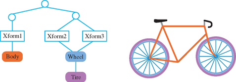
A scene graph can be thought of as a more sophisticated version of a display list. It is a data structure containing the information that represents the scene. But instead of simply holding a linear sequence of OpenGL commands the nodes of a scene graph can hold whatever data and procedures are needed to manipulate or render the scene. It is a directed graph, rather than a list. This topology is used to collect elements of the scene into hierarchical groupings. The organization of scene graphs is often spatial in nature. Objects close to each other in the scene graph are close to each other physically. This supports efficient implementations of culling techniques such as view-frustum and portal culling. Figure 21.1 shows a schematic figure of a simple scene graph storing transforms and collections of geometric primitives that form objects. Note that a single object can be transformed multiple times to create multiple instances on the screen. This turns the scene graph from a simple tree structure to a directed acyclic graph (DAG).
In addition to objects, which correspond to items in the scene, attribute values and procedures can also be included as nodes in the scene graph. In the most common approach, nodes closer to the root of the graph are more global to the scene, affecting the interpretation of their child nodes. The graph topology can be changed to represent scene changes, and it can be traversed. Traversal makes it possible to easily update node information, or to use that information to generate the stream of OpenGL commands necessary to render it.
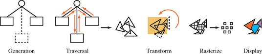
This type of organization is general enough that an application can use the scene graph for tasks that require information about spatial relationships but that do not necessarily involve graphics. Example include computing 3D sound sources, and source data for collision detection. Since it is such a common approach, this chapter discussess graphics processing steps in the context of an application using a scene graph. This yields a five-stage process. It starts with application generating or modifying scene graph elements and ends with OpenGL updating the framebuffer. The stages are illustrated in Figure 21.2. It shows the states of the pipeline, with data and commands proceeding from left to right. The following sections describe each stage and what system attributes affect its performance.
Generation
During the generation stage, object and attribute data is created or updated by the application. The possible types, purpose, and updating requirements of the graphics data are as varied as the graphics applications themselves. The object data set can be updated to reflect changes in position or appearance of objects, or annotated with application-specific information to support spatially based techniques such as 3D sound and collision detection.
For a scene graph-based application, the generation phase is where nodes are added, removed, or updated by the application to reflect the current state of the scene. The interconnections between nodes can change to reflect changes in their relationship.
As a simple example, consider a scene graph whose nodes only contain geometry or a transform. A new object can be created by adding nodes to the scene graph: geometry to represent the object (or components of a complex object) and the transforms needed to position and orient it. The generation phase is complete when the scene graph has been updated to reflect the current state of the scene. In general, performance of this stage depends on system (CPU, memory) performance, not the performance of the graphics hardware.
Traversal
The traversal stage uses the data updated by the generation stage. Here, the graphics-related data set is traversed to generate input data for later stages. If the data is organized as a scene graph, the graph itself is traversed, examining each element to extract the information necessary to create the appropriate OpenGL commands. Procedures linked to the graph are run as they are encountered, generating data themselves or modifying existing data in the graph. Traversal operations can be used to help implement many of the techniques described here that have object-space components (such as reflections, shadowing, and visibility culling), because the scene graph contains information about the spatial relationships between objects in the scene.
Traversing the simple example scene graph shown in Figure 21.1 only generates OpenGL commands. Commands to update the modelview matrix are generated as each transform is encountered, and geometry commands such as glBegin/glEnd sequences, vertex arrays, or display lists are issued as geometry nodes are traversed. Even for this simple example the traversal order can be used to establish a hierarchy: transforms higher in the graph are applied first, changing the effect of transforms lower in the graph. This relationship can be implemented by pushing the transform stack as the traversal goes down the graph, popping as the traversal goes back up.
Since OpenGL has no direct support for scene graphs, the stages described up to this point must be implemented by the application or a scene graph library. However, in an application that has very limited requirements, an OpenGL display list or vertex array can be used to store the graphics data instead. It can be updated during the generation phase. In this case, the traversal step may only require rendering the stored data, which might be performed solely by the OpenGL implementation.
Executing an OpenGL display list can be considered a form of traversal. Since OpenGL display lists can contain calls to other OpenGL display lists, a display list can also form a DAG. Executing a display list walks the DAG, performing a depth-first traversal of the graph. The traversal may be executed on the host CPU, or in some advanced OpenGL implementations, parts of the traversal may be executed in the accelerator itself. Creating new display lists can be similarly thought of as a form of generation.
If the traversal stage is done in the application, performance of this stage depends on either the bandwidth available to the graphics hardware or system performance, depending on which is the limiting factor. If traversal happens within OpenGL, the performance details will be implementation dependent. In general, performance depends on the bandwidth available between the stored data and the rendering hardware.
Transform
The transform stage processes primitives, and applies transforms, texture coordinate generation, clipping, and lighting operations to them. From this point on, all update stages occur within the OpenGL pipeline, and the behavior is strictly defined by the specification. Although the transform stage may not be implemented as a distinct part of the implementation, the transformation stage is still considered separately when doing performance analysis. Regardless of the implementation details, the work the implementation needs to do in order to transform and light incoming geometry in this stage is usually distinct from the work done in the following stages. This stage will affect performance as a function of the number of triangles or vertices on the screen and the number of transformations or other geometry state updates in the scene.
Rasterization
At this stage, higher-level representations of geometry and images are broken down into individual pixel fragments. Since this stage creates pixel fragments, its performance is a function of the number of fragments created and the complexity of the processing on each fragment. For the purposes of performance analysis it is common to include all of the steps in rasterization and fragment processing together. The number of active texture units, complexity of a fragment programs, framebuffer blending, and depth testing can all have a significant influence on performance. Not all pixels created by rasterizing a triangle may actually update the framebuffer, because alpha, depth, and stencil testing can discard them. As a result, framebuffer update performance and rasterization performance aren’t necessarily the same.
Display
At the display stage, individual pixel values are scanned from the color buffer and transmitted to the display device. For the most part the display stage has limited influence on the overall performance of the application. However, some characteristics (such as locking to the video refresh rate) can significantly affect the performance of an application.
21.1.2 Vertex Updates
A key factor affecting update performance that can be controlled by the application is the efficiency of vertex updates. Vertex updates occur during the traversal stage, and are often limited by system bandwidth to the graphics hardware. Storing vertex information in vertex arrays removes much of the function call overhead associated with glBegin/glEnd representations of data. Vertex arrays also make it possible to combine vertex data into contiguous regions, which improves transfer bandwidth from the CPU to the graphics hardware. Although vertex arrays reduce overhead and improve performance, their benefits come at a cost. Their semantics limit their ability to improve a bandwidth-limited application.
Ideally, vertex arrays make it possible to copy vertex data “closer” to the rendering hardware or otherwise optimize the placement of vertex data to improve performance. The original (OpenGL 1.1) definition prevents this, however. The application “owns” the pointer to the vertex data, and the specification semantics prevents the implementation from reusing cached data, since it has no way to know or control when the application modifies it. A number of vendor-specific extensions have been implemented to make caching possible, such as NV_vertex_array_range and ATI_vertex_array_object. This has culminated in a cross-vendor extension ARB_vertex_buffer_object, integrated into the core specification as part of OpenGL 1.5.
Display lists are another mechanism allowing the implementation to cache vertex data close to the hardware. Since the application doesn’t have access to the data after the display list is compiled, the implementation has more opportunities to optimize the representation and move it closer to the hardware. The requirement to change the OpenGL state as the result of display list execution can limit the ability of the OpenGL implementation to optimize stored display list representations, however. Any performance optimizations applied to display list data are implementation dependent. The developer should do performance experiments with display lists, such as segmenting geometry, state changes, and transform commands into separate display lists or saving and restoring transform state in the display list to find the optimal performance modes.
Regardless of how the vertex data is passed to the implementation, using vertex representations with a small memory footprint can improve bandwidth. For example, in many cases normals with type GL_UNSIGNED_SHORT will take less transfer time than normals with GL_FLOAT components, and be precise enough to generate acceptable results. Minimizing the number of vertex parameters, such as avoiding use of glTexCoord through the use of texture coordinate generation, also reduces vertex memory footprint and improves bandwidth utilization.
21.1.3 Texture Updates
Like vertex updates, texture updates can significantly influence overall performance, and should be optimized by the application. Unlike vertex updates, OpenGL has always had good support for caching texture data close to the hardware. Instead of finding ways to cache texture data, the application’s main task becomes managing texture updates efficiently. A key approach is to incrementally update textures, spreading the update load over multiple frames whenever possible. This reduces the peak bandwidth requirements of the application. Two good candidates for incremental loads are mipmapped textures, and large “terrain” textures. For many applications, only parts of these types of textures are visible at any given time.
A mipmapped textured object often first comes into view at some distance from the viewer. Usually only coarser mipmap levels are required to texture it at first. As the object and viewer move closer to each other, progressively finer mipmap levels are used. An application can take advantage of this behavior by loading coarser mipmap levels first and then progressively loading finer levels over a series of frames. Since coarser levels are low resolution, they take very little bandwidth to load. If the application doesn’t have the bandwidth available to load finer levels fast enough as the object approaches, the coarser levels provide a reasonable fallback.
Many large textures have only a portion of their texture maps visible at any given time. In the case where a texture has higher resolution than the screen, it is impossible to show the entire texture at level 0, even if it is viewed on edge. An edge on a non-mipmapped texture will be only coarsely sampled (not displaying most of its texels) and will show aliasing artifacts. Even a mipmapped texture will blur down to coarser texture levels with distance, leaving only part of level 0 (the region closest to the viewer) used to render the texture.
This restriction can be used to structure large texture maps, so that only the visible region and a small ring of texture data surrounding it have to be loaded into texture memory at any given time. It breaks up a large texture image into a grid of uniform texture tiles, and takes advantage of the properties of wrapped texture coordinates. Section 14.6 describes this technique, called texture paging, in greater detail.
21.2 Managing Frame Time
An interactive graphics application has to perform three major tasks: receive new input from the user, perform the calculations necessary to draw a new frame, and send update and rendering instructions to the hardware. Some applications, such as those used to simulate vehicles or sophisticated games, have very demanding latency and performance requirements. In these applications, it can be more important to maintain a constant frame rate than to update as fast as possible. A varying frame rate can undermine the realism of the simulation, and even lead to “simulator sickness,” causing the viewer to become nauseous. Since these demanding applications are often used to simulate an interactive visual world, they are often called visual simulation (a.k.a. “vissim”) applications.
Vissim applications often have calculation and rendering loads that can vary significantly per frame. For example, a user may pan across the scene to a region of high depth complexity that requires significantly more time to compute and render. To maintain a constant frame rate, these applications are allotted a fixed amount of time to update a scene. This time budget must always be met, regardless of where the viewer is in the scene, or the direction the viewer is looking. There are two ways to satisfy this requirement. One approach is to statically limit the geometry and texture data used in the application while the application is being written. Typically, these limits have to be severe in order to handle the worst case. It can also be difficult to guarantee there is no view position in the scene that will take too long to render. A more flexible approach is for the application to dynamically restrict the amount of rendering work, controlling the amount of time needed to draw each frame as the application is running. Rendering time can be managed by simplifying or skipping work in the generation and traversal stages and controlling the number and type of OpenGL commands sent to the hardware during the rendering stage.
There are three components to frame time management: accurately measuring the time it takes to draw each frame, adjusting the amount of work performed to draw the current frame (based on the amount of time it took to draw previous frames), and maintaining a safety margin of idle time at the end of all frames in order to handle variations. In essence, the rendering algorithm uses a feedback loop, adjusting the amount of rendering work from the time it took to draw the previous frames, adjusting to maintain a constant amount of idle time each frame (see Figure 21.3).
This frame management approach requires that the work a graphics application does each frame is ordered in a particular way. There are two criteria: critical work must be ordered so that it is always performed and the OpenGL commands must be started as early as possible. In visual simulation applications, taking into account the user input and using it to update the viewer’s position and orientation are likely to be the highest-priority tasks. In a flight simulation application, for example, it is critical that the view out of the windshield respond accurately and quickly to pilot inputs. It would be better to drop distant frame geometry than to inconsistently render the viewer’s position. Therefore, reading input must be done consistently every frame.
Starting OpenGL commands early in the frame requires that this task be handled next. This is done to maximize parallelism. Most graphics hardware implementations are pipelined, so a command may complete asynchronously some time after it is sent. A visual simulation application can issue all of its commands, and then start the computation work necessary to draw the next frame while the OpenGL commands are still being rendered in the graphics hardware. This ordering provides some parallelism between graphics hardware and the CPU, increasing the work that can be done each frame. This is why calculations for the next frame are done at the end of the current frame.
Because of parallelism, there are two ways frame time can be exceeded: too many OpenGL commands have been issued (causing the hardware to take too long to draw the frame) or the calculation phase can take too long, exceeding the frame time and interfering with the work that needs to be completed during the next frame. Having the calculation phase happen last makes it easier to avoid both problems. The amount of idle time left during the previous frame can be used to adjust the amount of OpenGL work to schedule for the next frame. The amount of time left in the current frame can be used to adjust the amount of calculation work that should be done. Note that using the previous frame’s idle time to compute the next frame’s OpenGL work introduces two frames of latency. This is necessary because the OpenGL pipeline may not complete its current rendering early enough for the calculation phase to measure the idle time.
Based on the previous criteria, the application should divide the work required to draw a scene into three main phases. At the start of each frame (after the buffer swap) the application should read the user inputs (and ideally use them to update the viewer’s position and orientation), send the OpenGL commands required to render the current frame, and perform the calculations needed to render the next frame. Note that the calculations done at the end of a given frame will affect the next frame, since the OpenGL commands rendering the current frame have already been issued. Ideally, these calculations are ordered so that low-priority ones can be skipped to stay within one frame time. The following sections describe each of the these three rendering phases in more detail.
21.2.1 Input Phase
The user input is read early in the frame, since updating input consistently is critical. It is important that the view position and orientation match the user input with as little “lag” as possible, so it is ideal if the user input is used to update the viewer position in the current frame. Fortunately, this is usually a fast operation, involving little more than reading control input positions and updating the modelview (and possibly the projection) transform. If multiple processors are available, or if the implementation of glClear is nonblocking, this task (and possibly other nongraphics work) can be accomplished while the framebuffer is being cleared at the beginning of the frame. If immediately updating the viewer position is not low cost, due to the structure of the program, another option is to use the input to update the viewer position during the start of the computation phase. This adds a single frame of latency to the input response, which is often acceptable. Some input latency is acceptable in a visual simulation application, as long as it is small and consistent. It can be a worthwhile trade-off if it starts the rendering phase sooner.
21.2.2 Rendering Phase
Once the user inputs are handled properly, the rendering phase should begin as early as possible. During this phase, the application issues the texture loads, geometry updates, and state changes needed to draw the scene. This task is a significant percentage of the total time needed to draw a frame, and it needs to be measured accurately. This can be done by issuing a glFinish as the last command and measuring the time from the start of the first command to the time the glFinish command completes. Since this is a synchronous operation, the thread executing this command stalls waiting for the hardware to finish. To maintain parallelism, the application issuing the OpenGL commands is usually in a separate execution thread. Its task is to issue a precomputed list of OpenGL commands, and measure the time it takes to draw them.
There are a number of ways to adjust the amount of time it takes to complete the rendering phase. The number of objects in the scene can be reduced, starting with the smallest and least conspicuous ones. Smaller, coarser textures can also be used, as well as restricting the number of texture LODs in use to just the coarser ones, saving the overhead of loading the finer ones. A single texture can be used to replace a number of similar ones. More complex time-saving techniques, such as geometry LOD, can also be used (see Section 16.4 for details on this technique).
21.2.3 Computation Phase
Ideally, every frame should start with the calculations necessary to create and configure the OpenGL rendering commands already completed. This minimizes the latency before the rendering pass can start. The computation phase performs this task ahead of time. After the rendering commands for a frame have been sent, the remaining frame time is used to perform the computations needed for the next frame. As mentioned previously, a multithreaded application can take advantage of hardware pipelining to overlap some of the rendering phase with the start of the computation phase. Care must be taken to ensure that the start of the calculation phase doesn’t steal cycles from the rendering thread. It must submit all of its OpenGL commands as early as possible.
This restriction may be relaxed in a multiprocessor or hyperthreading system. If it doesn’t impact the rendering work, the computation and rendering phases can start at the same time, allowing more computation to be done per frame.
There might not be enough time in the computation phase to perform all calculations. In this case, some computations will have to be deferred. In general, some computations must be done every frame, others will have a lower priority and be done less often. In order to decide which computations are less important, they can be sorted based on how they affect the scene. Computations can be categorized by how viewer dependent they are. Viewer dependence is a measure of how strongly correlated the computation is to viewer position and orientation. The more viewer dependent a computation is the more sensitive it is to stale input, and the more likely it will produce incorrect results if it is deferred. The most viewer-dependent computations are those that generate viewer position transforms. The time between when the user inputs are read and the time these computations are updated should be kept small, no more than one or two frames. Significant latency between updates will be noticeable to the user, and can impact the effectiveness of the visual simulation application.
On the other hand, many calculations are only weakly viewer dependent. Calculations such as geometric LOD (Section 16.4), some types of scene graph updates, view culling, and so on can affect rendering efficiency, but only change the rendered scene slightly if they are computed with stale input values. This type of work can be computed less often in order to meet frame time constraints.
As with all phases of frame updates, a visual simulation application should use all of the computation time available without compromising the frame rate. Since there can be some latency between the time the buffer swap command is called and the next frame refresh, an application can potentially use that time to do additional computations. This time is available if the implementation provides a nonblocking swap command, or if the swap command is executed in a thread separate from the one doing the computation.
21.2.4 The Safety Margin
Like the rendering phase, the calculation phase has to be managed to maintain a constant frame rate. As with rendering, this is done by prioritizing the work to be done, and stopping when the time slice runs out. If the calculations run even a little too long, the frame swap will be missed, resulting in a noticeable change in update rate (see Section 21.3.3 for details on this phenomenon). Not all calculation or rendering work is fine grained, so a safety margin (a period of dead time) is reserved for the end of each frame. If the rendering and calculation phases become long enough to start to significantly reduce the amount of safety margin time, the amount of work done in the next frame is cut back. If the work completes early, increasing the amount of safety margin time, the work load is incrementally increased. This creates a feedback loop, where the per-frame is adjusted to match the changing amount of rendering and calculating needed to be done to render the current view.
21.3 Application Performance Tuning
Any graphics application that has high performance requirements will require performance tuning. Graphics pipeline implementations, whether they are hardware or software based, have too many implementation-specific variations to make it possible to skip a tuning step. The rendering performance of the application must be measured, the bottlenecks found, and the application adjusted to fix them.
Maximizing the performance of a graphics application is all about finding bottlenecks; i.e., localized regions of the application code that are restricting performance. Like debugging an application, locating and understanding bottlenecks is usually more difficult than fixing them. This section begins by discussing common bottlenecks in graphics applications and some useful techniques for fixing them. It also discusses ways of measuring applications so that their performance characteristics are understood and their bottlenecks are identified. Multithreaded OpenGL applications are also discussed, including some common threading architectures that can improve an application’s performance.
21.3.1 Locating Bottlenecks
As mentioned previously, tuning an application is the process of finding and removing bottlenecks. A bottleneck is a localized region of software that can limit the performance of the entire application. Since these regions are usually only a small part of the overall application, and not always obvious, it’s rarely productive to simply tune parts of the application that appear “slow” from code inspection. Bottlenecks should be found by measuring (benchmarking) the application and analyzing the results.
In traditional application tuning, finding bottlenecks in software involves looking for “inner loops,” the regions of code most often executed when the program is running. Optimizing this type of bottleneck is important, but graphics tuning also requires knowledge of the graphics pipeline and its likely bottlenecks. The graphics pipeline consists of three conceptual stages. Except for some very low-end systems, it’s common today for all or part of the last two stages to be accelerated in hardware. In order to achieve maximum performance, the pipeline must be “balanced”—each stage of the pipeline must be working at full capacity.
This is not always easy to do, since each stage of the pipeline tends to produce more output for the following stage than it received from the previous one. When designing hardware, pipeline stages are sized to handle this amplification of work for “typical” cases, but the amount of work produced in each stage depends on the command stream that the application sends to the hardware. The stages are rarely in balance unless the application has been performance tuned.
The conceptual pipeline subsystems are:
• The application subsystem (i.e., the application itself) feeds the OpenGL implementation by issuing commands to the geometry subsystem.
• The geometry subsystem performs per-vertex operations such as coordinate transformations, lighting, texture coordinate generation, and clipping. The processed vertices are assembled into primitives and sent to the raster subsystem.
• The raster subsystem performs per-pixel operations—from simple operations such as writing color values into the framebuffer, to more complex operations such as texture mapping, depth buffering, and alpha blending.
To illustrate how the amount of work done by each pipeline stage depends on the application, consider a program that draws a small number of large polygons. Since there are only a few polygons, the geometry subsystem is only lightly loaded. However, those few polygons cover many pixels on the screen, so the load on the raster subsystem is much higher. If the raster subsystem can’t process the triangles as fast as the geometry subsystem is feeding them, the raster subsystem becomes a bottleneck. Note that this imbalance cannot be determined solely from static analysis of the application. Many graphics systems have very powerful raster engines. The hypothesis that the raster subsystem is limiting the speed of the program must be proved through benchmarking and performance experiments.
To avoid a rasterization bottleneck, the work between the geometry and rasterization stages must be balanced. One way to do this is to reduce the work done in the raster subsystem. This can be done by turning off modes such as texturing, blending, or depth buffering. Alternatively, since spare capacity is available in the geometry subsystem more work can be performed there without degrading performance. A more complex lighting model could be used, or objects can be tessellated more finely to create a more accurate geometric model.
21.3.2 Finding Application Bottlenecks
Graphics bottlenecks can usually be fixed by rebalancing the pipeline stages, but the more difficult part is determining where the bottleneck is located. The performance of each pipeline stage depends on the design of the OpenGL hardware and software, and the pattern of commands being processed. The resulting performance characteristics can be quite complex. Additional complexity can result because a bottleneck in an early stage of the pipeline can change the behavior of later stages.
The basic strategy for isolating bottlenecks is to measure the time it takes to execute part or all of the program and then change the code in ways that add or subtract work at a single point in the graphics pipeline. If changing the amount of work done by a given stage does not alter performance appreciably, that stage is not the bottleneck. Conversely, a noticeable difference in performance indicates a bottleneck. Since bottlenecks early in the pipeline can mask later ones, check for early bottlenecks first. Table 21.1 provides an overview of factors that may limit rendering performance, and names the part of the pipeline to which they belong.
Table 21.1
Factors Influencing Performance
| Performance Parameter | Pipeline Stage |
| Amount of data per polygon | All stages |
| Application overhead | Application |
| Transform rate and geometry mode setting | Geometry subsystem |
| Total number of polygons in a frame | Geometry and raster subsystem |
| Number of pixels filled | Raster subsystem |
| Fill rate for the current mode settings | Raster subsystem |
| Duration of screen and/or depth buffer clear | Raster subsystem |
Application Subsystem Bottlenecks
The first potential bottleneck can come if the application doesn’t issue OpenGL commands to the hardware fast enough. To measure the performance of the application accurately, the OpenGL calls can be “stubbed out.” Stubbing out an OpenGL call means using an empty function call in place of the real OpenGL command. The application with stubs can then be benchmarked to measure its maximum performance.
To get an accurate assessment of the application’s performance, the behavior of the application should be preserved by attempting to keep the number of instructions executed and the way memory is accessed unchanged. Since some OpenGL commands are used much more often than others, stubbing just a few key commands may be sufficient. For example, if the application uses glBegin/glEnd sequences to render geometry, replacing the vertex and normal calls glVertex3fv and glNormal3fv with color subroutine calls (glColor3fv) preserves the CPU behavior while eliminating all drawing and lighting work in the graphics pipeline. If making these changes does not significantly improve the time taken to render a frame, the application is the bottleneck.
On many faster hardware accelerators, the bus between the CPU and the graphics hardware can limit the number of polygons sent from the application to the geometry subsystems. To test for this bottleneck, reduce the amount of data being sent per vertex. For example, if removing color and normal parameters from the vertices shows a speed improvement the bus is probably the bottleneck.
Geometry Subsystem Bottlenecks
Applications that suffer from bottlenecks in the geometry subsystem are said to be transform limited (or sometimes geometry limited). To test for bottlenecks in geometry operations, change the application so that it issues the same number of commands and fills the same number of pixels but reduces the amount of geometry work. For example, if lighting is enabled, call glDisable with a GL_LIGHTING argument to temporarily turn it off. If performance improves, the application has a geometry bottleneck. Transformation and clipping performance can be measured in a similar fashion. All transforms can be set to identity, and all application-defined clipping planes can be disabled. Geometry can also be altered so that no clipping is needed to render it. Measuring geometry performance with this method can be tricky. Some hardware implementations are configured to run full speed over a wide range of geometry configurations, and changes to the geometry subsystem can inadvertently change the load of the raster subsystem. Understanding the hardware’s performance profile is important in avoiding fruitless attempts to tune geometry processing.
Rasterization Subsystem Bottlenecks
Applications that cause bottlenecks at the rasterization (per-pixel) stage in the pipeline are said to be fill limited. To test for bottlenecks in rasterization operations, shrink objects or make the window smaller to reduce the number of pixels being processed. This technique will not work if the program alters its behavior based on the sizes of objects or the size of the window. Per-pixel work can also be reduced by turning off operations such as depth buffering, texturing, or alpha blending. If any of these experiments speed up the program, it has a fill bottleneck. Like geometry state changes discussed in the previous section, consider that the hardware implementation may not slow down for certain rasterization state changes.
At the rasterization stage, performance may strongly depend on the type of primitive being rendered. Many programs draw a variety of primitives, each of which stresses a different part of the system. Decompose such a program into homogeneous pieces and time each one separately. After measuring these results, the slowest primitive type can be identified and optimized.
Oversubscribing texture memory resources can also cause significant performance degradation. Texture memory thrashing can be tested for by temporarily reducing the number of different textures in use. Other rasterization and fragment processing-related state changes can also adversely affect performance. These can be difficult to locate. Tools that trace and gather statistics on the number and types of OpenGL commands issued each frame can be invaluable in understanding the load generated by an application.
Optimizing Cache and Memory Usage
On most systems, memory is structured in a hierarchy that contains a small amount of fast, expensive memory at the top (e.g., CPU registers) through a series of larger and slower storage caches to a large amount of slow storage at the base (e.g., system memory). As data is referenced, it is automatically copied into higher levels of the hierarchy, so data that is referenced most often migrates to the fastest memory locations.
The goal of machine designers and programmers is to improve the likelihood of finding needed data as high up in this memory hierarchy as possible. To achieve this goal, algorithms for maintaining the hierarchy (embodied in the hardware and the operating system) assume that programs have locality of reference in both time and space. That is, programs are much more likely to access a location that has been accessed recently or is close to another recently accessed location. Performance increases if the application is designed to maximize the degree of locality available at each level in the memory hierarchy.
Minimizing Cache Misses
Most CPUs have first-level instruction and data caches on chip. Many also have second-level caches that are bigger but somewhat slower. Memory accesses are much faster if the data is already loaded into the first-level cache. When a program accesses data that is not in one of the caches, a cache miss occurs. This causes a block of consecutively addressed words, including the data the program just tried to access, to be loaded into the cache. Since cache misses are costly, they should be minimized. Cache misses can be minimized by using the following techniques.
• Keep frequently accessed data together. Store and access frequently used data in flat, sequential data structures and avoid pointer indirection. This way, the most frequently accessed data remains in the first-level cache as much as possible.
• Access data sequentially. Each cache miss brings in a block of consecutively addressed words of needed data. If the program is accessing data sequentially, each cache miss will bring in n words at a time, improving bandwidth (the exact value of n is system dependent). If only every nth word is accessed (strided access) the cache constantly brings in unneeded data, degrading performance.
• Avoid simultaneously traversing several large buffers of data, such as an array of vertex coordinates and an array of colors within a loop. This behavior can cause cache aliasing between the buffers. Instead, pack the contents into one buffer whenever possible. If the application uses vertex arrays, try to use interleaved arrays.
Some framebuffers have cache-like behaviors as well. The application can utilize this caching by ordering geometry so that drawing the geometry causes writes to adjacent regions of the screen. Using connected primitives such as triangle and line strips tends to create this behavior, and offers other performance advantages by minimizing the number of vertices needed to represent a continuous surface.
Modern graphics accelerators make heavy use of caching for vertex and texture processing. Use of indexed vertex arrays with careful ordering of vertex attributes and indices can substantially improve vertex cache hit rates. Applications have less control over texture cache performance, but programmable fragment programs provide substantial flexibility in how texture coordinates are computed. Dependent texture reads, environment mapping, and other texture coordinate computations can suffer from poor locality.
Storing Data in an Efficient Format
The design effort required to create a simpler graphics database can make a significant difference when traversing that data for display. A common tendency is to leave the data in a format that is optimized for loading or generating the object, but suboptimal for actually displaying it. For peak performance, do as much work as possible before rendering. This preprocessing is typically performed when an application can temporarily be noninteractive, such as at initialization time or when changing from a modeling to a fast-rendering mode.
Minimizing State Changes
A graphics application will almost always benefit if the number of state changes is reduced. A good way to do this is to sort scene data according to what state values are set and render primitives with the same state settings together. Mode changes should be ordered so that the most expensive state changes occur least often. Although it can vary widely with implementation, typically it is expensive to change texture binding, material parameters, fog parameters, texture filter modes, and the lighting model.
Measurement is the best way to determine which state settings are most expensive on a particular implementation. On systems that fully accelerate rasterization, for example, it may not be expensive to change rasterization controls such as enabling depth testing or changing the comparison function. On a system using software rasterization, however, these state changes may cause a cached graphics state, such as function pointers or automatically generated code, to be flushed and regenerated.
An OpenGL implementation may not optimize state changes that are redundant, so it is also important for the application to avoid setting the same state values multiple times. Sometimes sorting rendering by state isn’t practical, and redundant state changes can result. In these situations, shadowing state changes and discarding (filtering) redundant changes can often improve performance.
21.3.3 Measuring Performance
When benchmarking any application, there are common guidelines that when followed help ensure accurate results. The system used to measure performance should be idle, rather than executing competing activities that could steal system resources from the application being measured. A good system clock should be used for measuring performance with sufficient resolution, low latency, and producing accurate, reproducible results. The measurements themselves should be repeated a number of times to average out atypical measurements. Any significant variation in measurements should be investigated and understood. Beyond these well-known practices, however, are performance techniques and concepts that are specific to computer graphics applications. Some of these fundamental ideas are described in the following, along with their relevance to OpenGL applications.
Video Refresh Quantization
A dynamic graphics application renders a series of frames in sequence, creating animated images. The more frames rendered per second the smoother the motion appears. Smooth, artifact-free animation also requires double buffering. In double buffering, one color buffer holds the current frame, which is scanned out to the display device by video hardware, while the rendering hardware is drawing into a second buffer that is not visible. When the new color buffer is ready to be displayed, the application requests that the buffers be swapped. The swap is delayed until the next vertical retrace period between video frames, so that the update process isn’t visible on the screen.
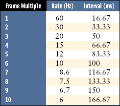
Frame rates must be integral multiples of the screen refresh time, 16.7 msec (milliseconds) for a 60-Hz display. If the rendering time for a frame is slightly longer than the time for n raster scans, the system waits until the n + 1st video period (vertical retrace) before swapping buffers and allowing drawing to continue. This quantizes the total frame time to multiples of the display refresh rate. For a 60-Hz refresh rate, frame times are quantized to (n + 1) * 16.7 msec. This means even significant improvements in performance may not be noticeable if the saving is less than that of a display refresh interval.
Quantization makes performance tuning more difficult. First, quantizing can mask most of the details of performance improvements. Performance gains are often the sum of many small improvements, which are found by making changes to the program and measuring the results. Quantizing may hide those results, making it impossible to notice program changes that are having a small but positive effect. Quantizing also establishes a minimum barrier to making performance gains that will be visible to the user. Imagine an application running fast enough to support a 40-fps refresh rate. It will never run faster than 30 fps on a 60-Hz display until it has been optimized to run at 60 fps, almost double its original rate. Table 21.2 lists the quantized frame times for multiples of a 60-Hz frame.
To accurately measure the results of performance changes, quantization should be turned off. This can be done by rendering to a single-buffered color buffer. Besides making it possible to see the results of performance changes, single-buffering performance also shows how close the application’s update rate is to a screen refresh boundary. This is useful in determining how much more improvement is necessary before it becomes visible in a double-buffered application. Double buffering is enabled again after all performance tuning has been completed.
Quantization can sometimes be taken advantage of in application tuning. If an application’s single-buffered frame rate is not close to the next multiple of a screen refresh interval, and if the current quantized rate is adequate, the application can be modified to do additional work, improving visual quality without visibly changing performance. In essence, the time interval between frame completion and the next screen refresh is being wasted, which it can be used instead to produce a richer image.
Finish Versus Flush
Modern hardware implementations of OpenGL often queue graphics commands to improve bandwidth. Understanding and controlling this process is important for accurate benchmarking and maximizing performance in interactive applications.
When an OpenGL implementation uses queuing, the pipeline is buffered. Incoming commands are accumulated into a buffer, where they may be stored for some period of time before rendering. Some queuing pipelines use the notion of a high water mark, deferring rendering until a given buffer has exceeded some threshold, so that commands can be rendered in a bandwidth-efficient manner. Queuing can allow some parallelism between the system and the graphics hardware: the application can fill the pipeline’s buffer with new commands while the hardware is rendering previous commands. If the pipeline’s buffer fills, the application can do other work while the hardware renders its backlog of commands.
The process of emptying the pipeline of its buffered commands is called flushing. In many applications, particularly interactive ones, the application may not supply commands in a steady stream. In these cases, the pipeline buffer can stay partially filled for long period of time, not rendering any more commands to hardware even if the graphics hardware is completely idle.
This situation can be a problem for interactive applications. If some graphics commands are left in the buffer when the application stops rendering to wait for input, the user will see an incomplete image. The application needs a way of indicating that the buffer should be emptied, even if it isn’t full. OpenGL provides the command glFlush to perform this operation. The command is asynchronous, returning immediately. It guarantees that outstanding buffers will be flushed and the pipeline will complete rendering, but doesn’t provide a way to indicate exactly when the flush will complete.
The glFlush command is inadequate for graphics benchmarking, which needs to measure the duration between the issuing of the first command and the completion of the last. The glFinish command provides this functionality. It flushes the pipeline, but doesn’t return until all commands sent before the finish have completed. The difference between finish and flush is illustrated in Figure 21.4
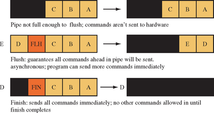
To benchmark a piece of graphics code, call glFinish at the end of the timing trial, just before sampling the clock for an end time. The glFinish command should also be called before sampling the clock for the start time, to ensure no graphics calls remain in the graphics queue ahead of the commands being benchmarked.
While glFinish ensures that every previous command has been rendered, it should be used with care. A glFinish call disrupts the parallelism the pipeline buffer is designed to achieve. No more commands can be sent to the hardware until the glFinish command completes. The glFlush command is the preferred method of ensuring that the pipeline renders all pending commands, since it does so without disrupting the pipeline’s parallelism.
21.3.4 Measuring Depth Complexity
Measuring depth complexity, or the number of fragments that were generated for each pixel in a rendered scene, is important for analyzing rasterization performance. It indicates how polygons are distributed across the framebuffer and how many fragments were generated and discarded—clues for application tuning. Depending on the performance details of the OpenGL implementation, depth complexity analysis can help illustrate problems that can be solved by presorting geometry, adding a visibility culling pass, or structuring parts of the scene to use a painters algorithm for hidden surface removal instead of depth testing.
One way to visualize depth complexity is to use the color values of the pixels in the scene to indicate the number of times a pixel is written. It is easy to do this using the stencil buffer. The basic approach is simple: increment a pixel’s stencil value every time the pixel is written. When the scene is finished, read back the stencil buffer and display it in the color buffer, color coding the different stencil values.
The stencil buffer can be set to increment every time a fragment is sent to a pixel by setting the zfail and zpass parameters of glStencil0p to GL_INCR, and setting the func argument of glStencilFunc to GL_ALWAYS. This technique creates a count of the number of fragments generated for each pixel, irrespective of the results of the depth test. If the zpass argument to glStencil0p is changed to GL_KEEP instead (the setting of the fail argument doesn’t matter, since the stencil function is still set to GL_ALWAYS), the stencil buffer can be used to count the number of fragments discarded after failing the depth test. In another variation, changing zpass to GL_INCR, and zfail to GL_KEEP, the stencil buffer will count the number of times a pixel was rewritten by fragments passing the depth test. The following is a more detailed look at the first method, which counts the number of fragments sent to a particular pixel.
1. Clear the depth and stencil buffer:glClear(GL_STENCIL_BUFFER_BIT | GL_DEPTH_BUFFER_BIT).
2. Enable stenciling:glEnable(GL_STENCIL_TEST).
3. Set up the proper stencil parameters:glStencilFunc(GL_ALWAYS, 0, 0) and glStencilOp(GL_KEEP, GL_INCR, GL_INCR).
5. Read back the stencil buffer with glReadPixels, using GL_STENCIL_INDEX as the format argument.
6. Draw the stencil buffer to the screen using glDrawPixels, with GL_COLOR_INDEX as the format argument.
The glPixelMap command can be used to map stencil values to colors. The stencil values can be mapped to either RGBA or color index values, depending on the type of color buffer. Color index images require mapping colors with glPixelTransferi, using the arguments GL_MAP_COLOR and GL_TRUE.
Note that this technique is limited by the range of values of the stencil buffer (0 to 255 for an 8-bit stencil buffer). If the maximum value is exceeded, the value will clamp. Related methods include using framebuffer blending with destination alpha as the counter, but this requires that the application not use framebuffer blending for other purposes.
21.3.5 Pipeline Interleaving
OpenGL has been specified with multithreaded applications in mind by allowing one or more separate rendering threads to be created for any given process. Thread programming in OpenGL involves work in the OpenGL interface library. This means GLX, WGL, or other interface library calls are needed. Each rendering thread has a single context associated with it. The context holds the graphics state of the thread. A context can be disconnected from one thread and attached to another. The target framebuffer of the rendering thread is sometimes called its drawable. There can be multiple threads rendering to a single drawable. For more information on the role of threads in the OpenGL interface libraries, see Section 7.2, which describes the interactions of the interface libraries in more detail.
Each thread can be thought of as issuing a separate stream of rendering commands to a drawable. OpenGL does not guarantee that the ordering of the streams of different threads is maintained. Every time a different thread starts rendering, the previous commands sent by other threads may be interleaved with commands from the new thread. However, if a context is released from one thread and attached to another; any pending commands from the old thread are applied before any commands coming from the new one.
Providing general guidelines for multithreaded programming is beyond the scope of this book. There are two common thread architectures, however, that are particularly useful for OpenGL applications and bear mentioning.
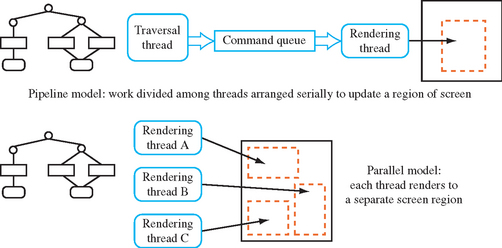
The first is the pipeline model. In this model, the application divides its graphics work into a series of pipeline stages, connected by queues. For example, one or more threads might update a scene graph, and one or more may be traversing it, pushing drawing commands into a queue. A single rendering thread can then read each command from the queue, and make the appropriate OpenGL calls. This model is useful for scene-graph-oriented applications, and is easy to understand. A variant of this model, used to optimize visual simulation applications, is discussed briefly in Section 21.3. In the visual simulation example, rendering is kept in a separate thread to allow parallelism between rendering work and the computations needed to render the next frame.
The other model is a parallel rendering model. This model has multiple rendering threads. Each rendering thread is receiving commands from a central source, such as a scene graph or other database, rendering to separate drawables or separate regions within a drawable. This model is useful if the application is rendering multiple separate versions of the same data, such as a modeling program that renders multiple views of the data. However, care must be taken to ensure that rendering commands such as window clears do not affect overlapping parts of the window. Both the pipeline and parallel rendering models are illustrated in Figure 21.5.
In either case, creating a multiple-thread model is only useful in certain situations. The most obvious case is where the system supports multiple CPUs, or one or more “hyperthreaded” ones. A hypertheaded CPU is a single physical CPU that is designed to act as if it contains multiple “virtual” processors. Even a single nonhyperthreaded CPU system can benefit from threading if it is possible for one or more tasks to be stalled waiting for data or user input. If the application splits the tasks into individual threads, the application can continue to do useful work even if some of its threads are stalled. Common cases where a rendering thread may stall are during a screen clear, or while waiting for a glFinish command to complete.
21.4 Summary
This chapter provided a background and an introduction to the techniques of graphics performance tuning. While there are many graphics-specific details covered here, the main idea is simple: create experiments and measure the results. Computer graphics hardware is complex and evolving. It’s not practical to make assumptions about its performance characteristics. This is true whether writing a fixed-function OpenGL program or writing vertex or fragment programs. Reading all of the performance documentation available on a particular vendor’s hardware accelerator and OpenGL implementation is still useful however. It can make your guesses more educated and help to target performance tuning experiments more accurately.