Scene Realism
Although a number of fields of computer graphics, such as scientific visualization and CAD, don’t make creating realistic images a primary focus, it is an important goal for many others. Computer graphics in the entertainment industry often strives for realistic effects, and realistic rendering has always been a central area of research. A lot of image realism can be achieved through attention to the basics: using detailed geometric models, creating high-quality surface textures, carefully tuning lighting and material parameters, and sorting and clipping geometry to achieve artifact-free transparency. There are limits to this approach, however. Increasing the resolution of geometry and textures can rapidly become expensive in terms of design overhead, as well as incurring runtime storage and performance penalties.
Applications usually can’t pursue realism at any price. Most are constrained by performance requirements (especially interactive applications) and development costs. Maximizing realism becomes a process of focusing on changes that make the most visual difference. A fruitful approach centers around augmenting areas where OpenGL has only basic functionality, such as improving surface lighting effects and accurately modeling the lighting interactions between objects in the scene.
This chapter focuses on the second area: interobject lighting. OpenGL has only a very basic interobject lighting model: it sums all of the contributions from secondary reflections in a single “ambient illumination” term. It does have many important building blocks, however (such as environment mapping) that can be used to model object interactions. This chapter covers the ambient lighting effects that tend to dominate a scene: specular and diffuse reflection between objects, refractive effects, and shadows.
17.1 Reflections
Reflections are one of the most noticeable effects of interobject lighting. Getting it right can add a lot of realism to a scene for a moderate effort. It also provides very strong visual clues about the relative positioning of objects. Here, reflection is divided into two categories: highly specular “mirror-like” reflections and “radiosity-like” interobject lighting based on diffuse reflections.
Directly calculating the physics of reflection using algorithms such as ray tracing can be expensive. As the physics becomes more accurate, the computational overhead increases dramatically with scene complexity. The techniques described here help an application budget its resources, by attempting to capture the most significant reflection effects in ways that minimize overhead. They maintain good performance by approximating more expensive approaches, such as ray tracing, using less expensive methods.
17.1.1 Object vs. Image Techniques
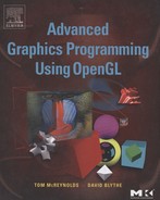
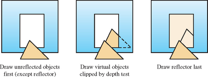
Consider a reflection as a view of a “virtual” object. As shown in Figure 17.1, a scene is composed of reflected objects rendered “behind” their reflectors, the same objects drawn in their unreflected positions, and the reflectors themselves. Drawing a reflection becomes a two-step process: using objects in the scene to create virtual reflected versions and drawing the virtual objects clipped by their reflectors.
There are two ways to implement this concept: image-space methods using textures and object-space approaches that manipulate geometry. Texture methods create a texture image from a view of the reflected objects, and then apply it to a reflecting surface. An advantage of this approach, being image-based, is that it doesn’t depend on the geometric representation of the objects being reflected. Object-space methods, by contrast, often must distort an object to model curved reflectors, and the realism of their reflections depends on the accuracy of the surface model. Texture methods have the most built-in OpenGL support. In addition to basic texture mapping, texture matrices, and texgen functionality, environment texturing support makes rendering the reflections from arbitrary surfaces relatively straightforward.
Object-space methods, in contrast, require much more work from the application. Reflected “virtual” objects are created by calculating a “virtual” vertex for every vertex in the original object, using the relationship between the object, reflecting surface, and viewer. Although more difficult to implement, this approach has some significant advantages. Being an object-space technique, its performance is insensitive to image resolution, and there are fewer sampling issues to consider. An object-space approach can also produce more accurate reflections. Environment mapping, used in most texturing approaches, is an approximation. It has the greatest accuracy showing reflected objects that are far from the reflector. Object-space techniques can more accurately model reflections of nearby objects. Whether these accuracy differences are significant, or even noticeable, depends on the details of the depicted scene and the requirements of the application.
Object-space, image-space, and some hybrid approaches are discussed in this chapter. The emphasis is on object-space techniques, however, since most image-space techniques can be directly implemented using OpenGL’s texturing functionality. Much of that functionality is covered in Sections 5.4 and 17.3.
Virtual Objects
Whether a reflection technique is classified as an object-space or image-space approach, and whether the reflector is planar or not, one thing is constant: a virtual object must be created, and it must be clipped against the reflector. Before analyzing various reflection techniques, the next two sections provide some general information about creating and clipping virtual objects.
Clipping Virtual Objects
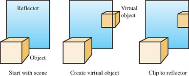
Proper reflection clipping involves two steps: clipping any reflected geometry that lies outside the edges of the reflected object (from the viewer’s point of view) and clipping objects that extend both in front of and behind the reflector (or penetrate it) to the reflector’s surface. These two types of clipping are shown in Figure 17.2. Clipping to a planar reflector is the most straightforward. Although the application is different, standard clipping techniques can often be reused. For example, user-defined clip planes can be used to clip to the reflector’s edges or surface when the reflection region is sufficiently regular or to reduce the area that needs to be clipped by other methods.
While clipping to a reflecting surface is trivial for planar reflectors, it can become quite challenging when the reflector has a complex shape, and a more powerful clipping technique may be called for. One approach, useful for some applications, is to handle reflection clipping through careful object modeling. Geometry is created that only contains the parts visible in the reflector. In this case, no clipping is necessary. While efficient, this approach can only be used in special circumstances, where the view position (but not necessarily the view direction), reflector, and reflected geometry maintain a static relationship.
There are also image-space approaches to clipping. Stencil buffering can be useful for clipping complex reflectors, since it can be used to clip per-pixel to an arbitrary reflection region. Rather than discarding pixels, a texture map of the reflected image can be constructed from the reflected geometry and applied to the reflecting object’s surface. The reflector geometry itself then clips an image of the virtual object to the reflector’s edges. An appropriate depth buffer function can also be used to remove reflecting geometry that extends behind the reflector. Note that including stencil, depth, and texture clipping techniques to object-space reflection creates hybrid object/image space approaches, and thus brings back pixel sampling and image resolution issues.
Issues When Rendering Virtual Objects
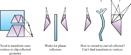
Rendering a virtual object properly has a surprising number of difficulties to overcome. While transforming the vertices of the source object to create the virtual one is conceptually straightforward when the reflector is planar, a reflection across a nonplanar reflector can distort the geometry of the virtual object. In this case, the original tessellation of the object may no longer be sufficient to model it accurately. If the curvature of a surface increases, that region of the object may require retessellation into smaller triangles. A general solution to this problem is difficult to construct without resorting to higher-order surface representations.
Even after finding the proper reflected vertices for the virtual object, finding the connectivity between them to form polygons can be difficult. Connectivity between vertices can be complicated by the effects of clipping the virtual object against the reflector. Clipping can remove vertices and add new ones, and it can be tedious to handle all corner cases, especially when reflectors have complex or nonplanar shapes.
More issues can arise after creating the proper geometry for the virtual object. To start, note that reflecting an object to create a virtual one reverses the vertex ordering of an object’s faces, so the proper face-culling state for reflected objects is the opposite of the original’s. Since a virtual object is also in a different position compared to the source object, care must be taken to light the virtual objects properly. In general, the light sources for the reflected objects should be reflected too. The difference in lighting may not be noticeable under diffuse lighting, but changes in specular highlights can be quite obvious.
17.1.2 Planar Reflectors
Modeling reflections across planar or nearly planar surfaces is a common occurrence. Many synthetic objects are shiny and flat, and a number of natural surfaces, such as the surface of water and ice, can often be approximated using planar reflectors. In addition to being useful techniques in themselves, planar reflection methods are also important building blocks for creating techniques to handle reflections across nonplanar and nonuniform surfaces.
Consider a model of a room with a flat mirror on one wall. To reflect objects in this planar reflector, its orientation and position must be established. This can be done by computing the equation of the plane that contains the mirror. Mirror reflections, being specular, depend on the position of both the reflecting surface and the viewer. For planar reflectors, however, reflecting the geometry is a viewer-independent operation, since it depends only on the relative position of the geometry and the reflecting surface. To draw the reflected geometry, a transform must be computed that reflects geometry across the mirror’s plane. This transform can be conceptualized as reflecting either the eye point or the objects across the plane. Either representation can be used; both produce identical results.
An arbitrary reflection transformation can be decomposed into a translation of the mirror plane to the origin, a rotation embedding the mirror into a major plane (for example the x − y plane), a scale of −1 along the axis perpendicular to that plane (in this case the z axis), the inverse of the rotation previously used, and a translation back to the mirror location.
Given a vertex P on the planar reflector’s surface and a vector V perpendicular to the plane, the reflection transformations sequence can be expressed as the following single 4 × 4 matrix R (Goldman, 1990):
Applying this transformation to the original scene geometry produces a virtual scene on the opposite side of the reflector. The entire scene is duplicated, simulating a reflector of infinite extent. The following section goes into detail on how to render and clip virtual geometry against planar reflectors to produce the effect of a finite reflector.
Clipping Planar Reflections
Reflected geometry must be clipped to ensure it is only visible in the reflecting surface. To do this properly, the reflected geometry that appears beyond the boundaries of the reflector from the viewer’s perspective must be clipped, as well as the reflected geometry that ends up in front of the reflector. The latter case is the easiest to handle. Since the reflector is planar, a single application-defined clipping plane can be made coplanar to the reflecting surface, oriented to clip out reflected geometry that ends up closer to the viewer.
If the reflector is polygonal, with few edges, it can be clipped with the remaining application clip planes. For each edge of the reflector, calculate the plane that is formed by that edge and the eye point. Configure this plane as a clip plane (without applying the reflection transformation). Be sure to save a clip plane for the reflector surface, as mentioned previously. Using clip planes for reflection clipping is the highest-performance approach for many OpenGL implementations. Even if the reflector has a complex shape, clip planes may be useful as a performance-enhancing technique, removing much of the reflected geometry before applying a more general technique such as stenciling.
In some circumstances, clipping can be done by the application. Some graphics support libraries support culling a geometry database to the current viewing frustum. Reflection clipping performance may be improved if the planar mirror reflector takes up only a small region of the screen: a reduced frustum that tightly bounds the screen-space projection of the reflector can be used when drawing the reflected scene, reducing the number of objects to be processed.
For reflectors with more complex edges, stencil masking is an excellent choice. There are a number of approaches available. One is to clear the stencil buffer, along with the rest of the framebuffer, and then render the reflector. Color and depth buffer updates are disabled, rendering is configured to update the stencil buffer to a specific value where a pixel would be written. Once this step is complete, the reflected geometry can be rendered, with the stencil buffer configured to reject updates on pixels that don’t have the given stencil value set.
Another stenciling approach is to render the reflected geometry first, and then use the reflector to update the stencil buffer. Then the color and depth buffer can be cleared, using the stencil value to control pixel updates, as before. In this case, the stencil buffer controls what geometry is erased, rather than what is drawn. Although this method can’t always be used (it doesn’t work well if interreflections are required, for example), it may be the higher performance option for some implementations: drawing the entire scene with stencil testing enabled is likely to be slower than using stencil to control clearing the screen. The following outlines the second approach in more detail.
1. Clear the stencil and depth buffers.
2. Configure the stencil buffer such that 1 will be set at each pixel where polygons are rendered.
3. Disable drawing into the color buffers using glColorMask.
4. Draw the reflector using blending if desired.
5. Reconfigure the stencil test using glStencilOp and glStencilFunc.
6. Clear the color and depth buffer to the background color.
8. Draw the rest of the scene (everything but the reflector and reflected objects).
The previous example makes it clear that the order in which the reflected geometry, reflector, and unreflected geometry are drawn can create different performance trade-offs. An important element to consider when ordering geometry is the depth buffer. Proper object ordering can take advantage of depth buffering to clip some or all of the reflected geometry automatically. For example, a reflector surrounded by nonreflected geometry (such as a mirror hanging on a wall) will benefit from drawing the nonreflected geometry in the scene first, before drawing the reflected objects. The first rendering stage will initialize the depth buffer so that it can mask out reflected geometry that goes beyond the reflector’s extent as it’s drawn, as shown in Figure 17.3. Note that the figure shows how depth testing can clip against objects in front of the mirror as well as those surrounding it. The reflector itself should be rendered last when using this method; if it is, depth buffering will remove the entire reflection, since the reflected geometry will always be behind the reflector. Note that this technique will only clip the virtual object when there are unreflected objects surrounding it, such as a mirror hanging on a wall. If there are clear areas surrounding the reflector, other clipping techniques will be needed.
There is another case that can’t be handled through object ordering and depth testing. Objects positioned so that all or part of their reflection is in front of the mirror (such as an object piercing the mirror surface) will not be automatically masked. This geometry can be eliminated with a clip plane embedded in the mirror plane. In cases where the geometry doesn’t cross the mirror plane, it can be more efficient for the application to cull out the geometry that creates these reflections (i.e., geometry that appears behind the mirror from the viewer’s perspective) before reflecting the scene.
Texture mapping can also be used to clip a reflected scene to a planar reflector. As with the previous examples, the scene geometry is transformed to create a reflected view. Next, the image of the reflected geometry is stored into a texture map (using glCopyTexImage2D, for example). The color and depth buffers are cleared. Finally, the entire scene is redrawn, unreflected, with the reflector geometry textured with the image of the reflected geometry. The process of texturing the reflector clips the image of the reflected scene to the reflector’s boundaries. Note that any reflected geometry that ends up in front of the reflector still has to be clipped before the texture image is created. The methods mentioned in the previous example, using culling or a clip plane, will work equally well here.
The difficult part of this technique is configuring OpenGL so that the reflected scene can be captured and then mapped properly onto the reflector’s geometry. The problem can be restated in a different way. In order to preserve alignment, both the reflected and unreflected geometry are rendered from the same viewpoint. To get the proper results, the texture coordinates on the reflector only need to register the texture to the original captured view. This will happen if the s and t coordinates correlate to x and y window coordinates of the reflector.
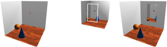
Rather than computing the texture coordinates of the reflector directly, the mapping between pixels and texture coordinates can be established using glTexGen and the texture transform matrix. As the reflector is rendered, the correct texture coordinates are computed automatically at each vertex. Configuring texture coordinate generation to GL_OBJECT_LINEAR, and setting the s, t and r coordinates to match one to one with x, y, and z in eye space, provides the proper input to the texture transform matrix. It can be loaded with a concatenation of the modelview and projection matrix used to “photograph” the scene. Since the modelview and projection transforms the map from object space to NDC space, a final scale-and-translate transform must be concatenated into the texture matrix to map x and y from [−1, 1] to the [0, 1] range of texture coordinates. Figure 17.4 illustrates this technique. There are three views. The left is the unreflected view with no mirror. The center shows a texture containing the reflected view, with a rectangle showing the portion that should be visible in the mirror. The rightmost view shows the unreflected scene with a mirror. The mirror is textured with the texture containing the reflected view. Texgen is used to apply the texture properly. The method of using texgen to match the transforms applied to vertex coordinates is described in more detail in Section 13.6.
The texture-mapping technique may be more efficient on some systems than stencil buffering, depending on their relative performance on the particular OpenGL implementation. The downside is that the technique ties up a texture unit. If rendering the reflector uses all available texture units, textured scenes will require the use of multiple passes.
Finally, separating the capture of the reflected scene and its application to the reflector makes it possible to render the image of the reflected scene at a lower resolution than the final one. Here, texture filtering blurs the texture when it is projected onto the reflector. Lowering resolution may be desirable to save texture memory, or to use as a special effect.
This texturing technique is not far from simply environment-mapping the reflector, using a environment texture containing its surroundings. This is quite easy to do with OpenGL, as described in Section 5.4. This simplicity is countered by some loss of realism if the reflected geometry is close to the reflector.
17.1.3 Curved Reflectors
The technique of creating reflections by transforming geometry can be extended to curved reflectors. Since there is no longer a single plane that accurately reflects an entire object to its mirror position, a reflection transform must be computed per-vertex. Computing a separate reflection at each vertex takes into account changes in the reflection plane across the curved reflector surface. To transform each vertex, the reflection point on the reflector must be found and the orientation of the reflection plane at that point must be computed.
Unlike planar reflections, which only depend on the relative positions of the geometry and the reflector, reflecting geometry across a curved reflector is viewpoint dependent. Reflecting a given vertex first involves finding the reflection ray that intersects it. The reflection ray has a starting point on the reflector’s surface and the reflection point, and a direction computed from the normal at the surface and the viewer position. Since the reflector is curved, the surface normal varies across the surface. Both the reflection ray and surface normal are computed for a given reflection point on the reflector’s surface, forming a triplet of values. The reflection information over the entire curved surface can be thought of as a set of these triplets. In the general case, each reflection ray on the surface can have a different direction.
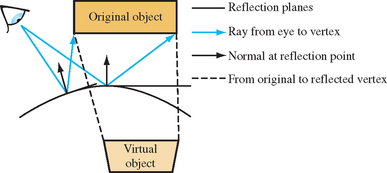
Once the proper reflection ray for a given vertex is found, its associated surface position and normal can be used to reflect the vertex to its corresponding virtual object position. The transform is a reflection across the plane, which passes through the reflection point and is perpendicular to the normal at that location, as shown in Figure 17.5. Note that computing the reflection itself is not viewer dependent. The viewer position comes into play when computing the reflection rays to find the one that intersects the vertex.
Finding a closed-form solution for the reflection point—given an arbitrary eye position, reflector position and shape, and vertex position—can be suprisingly difficult. Even for simple curved reflectors, a closed-form solution is usually too complex to be useful. Although beyond the scope of this book, there has been interesting research into finding reflection point equations for the class of reflectors described as implicit equations. Consult references such as Hanrahan (1992) and Chen (2000 and 2001) for more information.
Curved Reflector Implementation Issues
There are a few issues to consider when using an object-based technique to model curved reflections. The first is tessellation of reflected geometry. When reflecting across a curved surface, straight lines may be transformed into curved ones. Since the reflection transform is applied to the geometry per-vertex, the source geometry may need to be tessellated more finely to make the reflected geometry look smoothly curved. One metric for deciding when to tessellate is to compare the reflection point normals used to transform vertices. When the normals for adjacent vertices differ sufficiently, the source geometry can be tessellated more finely to reduce the difference.
Another problem that arises when reflecting geometry against a curved reflector is dealing with partially reflected objects. An edge may bridge two different vertices: one reflected by the curved surface and one that isn’t. The ideal way to handle this case is to find a transform for the unreflected point that is consistent with the reflected point sharing an edge with it. Then both points can be transformed, and the edge clipped against the reflector boundary.
For planar reflectors, this procedure is simple, since there is only one reflection transform. Points beyond the edge of the reflector can use the transform, so that edges clipped by the reflector are consistent. This becomes a problem for nonplanar reflectors because it may be difficult or impossible to extend the reflector and construct a reasonable transform for points beyond the reflector’s extent. This problem is illustrated in Figure 17.6.
Reflection boundaries also occur when a reflected object crosses the plane of the reflector. If the object pierces the reflector, it can be clipped to the surface, although creating an accurate clip against a curved surface can be computationally expensive. One possibility is to use depth buffering. The reflector can be rendered to update the depth buffer, and then the reflected geometry can be rendered with a GL_GREATER depth function. Unfortunately, this approach will lead to incorrect results if any reflected objects behind the reflector obscure each other. When geometry needs to be clipped against a curved surface approximated with planar polygons, application-defined clip planes can also be used.
Arbitrary Curved Reflectors
A technique that produces reflections across a curved surface is most useful if it can be used with an arbitrary reflector shape. A flexible approach is to use an algorithm that represents a curved reflector approximated by a mesh of triangles. A simple way to build a reflection with such a reflector is to treat each triangle as a planar reflector. Each vertex of the object is reflected across the plane defined by one or more triangles in the mesh making up the reflector. Finding the reflection plane for each triangle is trivial, as is the reflection transform.
Even with this simple method, a new issue arises: for a given object vertex, which triangles in the reflector should be used to create virtual vertices? In the general case, more than one triangle may reflect a given object vertex. A brute-force approach is to reflect every object vertex against every triangle in the reflector. Extraneous virtual vertices are discarded by clipping each virtual vertex against the triangle that reflected it. Each triangle should be thought of a single planar mirror and the virtual vertices created by it should be clipped appropriately. This approach is obviously inefficient. There are a number of methods that can be used to match vertices with their reflecting triangles. If the application is using scene graphs, it may be convenient to use them to do a preliminary culling/group step before reflecting an object. Another approach is to use explosion maps, as described in Section 17.8.
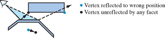
Reflecting an object per triangle facet produces accurate reflections only if the reflecting surface is truly represented by the polygon mesh; in other words, when the reflector is faceted. Otherwise, the reflected objects will be inaccurate. The positions of the virtual vertices won’t match their correct positions, and some virtual vertices may be missing, falling “between the cracks” because they are not visible in any triangle that reflected them, as shown in Figure 17.7.
This method approximates a curved surface with facets. This approximation may be adequate if the reflected objects are not close to the reflector, or if the reflector is highly tessellated. In most cases, however, a more accurate approximation is called for. Instead of using a single facet normal and reflection plane across each triangle, vertex normals are interpolated across the triangle.
The basic technique for generating a reflected image is similar to the faceted reflector approach described previously. The vertices of objects to be reflected must be associated with reflection points and normals, and a per-vertex reflection transform is constructed to reflect the vertices to create a “virtual” (reflected) object. The difference is that the reflection rays, normals, and points are now parameterized.
Parameterizing each triangle on the reflector is straightforward. Each triangle on the reflector is assumed to have three, possibly nonparallel, vertex normals. Each vertex and its normal is shared by adjacent triangles. For each vertex, vertex normal, and the eye position, a per-vertex reflection vector is computed. The OpenGL reflection equation, R = U − 2NT(N · U), can be used to compute this vector.
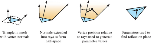
The normals at each vertex of a triangle can be extended into a ray, creating a volume with the triangle at its base. The position of a point within this space relative to these three rays can be used to generate parameters for interpolating a reflection point and transform, as illustrated in Figure 17.8.
Computing the distance from a point to each ray is straightforward. Given a vertex on the triangle V, and it’s corresponding normal N, a ray R can be defined in a parametric form as
Finding the closest distance from a point P to R is done by computing t for the point on the ray closest to P and then measuring the distance between P and that point. The formula is
This equation finds the value of t where P projects onto R. Since the points on the three rays closest to P form a triangle, the relationship between P and that triangle can be used to find barycentric coordinates for P. In general, P won’t be coplanar with the triangle. One way to find the barycentric coordinates is to project P onto the plane of the triangle and then compute its barycentric coordinates in the traditional manner.
The barycentric coordinates can be used to interpolate a normal and position from the vertices and vertex normals of the reflector’s triangle. The interpolated normal and position can be used to reflect P to form a vertex of the virtual object.
This technique has a number of limitations. It only approximates the true position of the virtual vertices. The less parallel the vertex normals of a triangle are the poorer the approximation becomes. In such cases, better results can be obtained by further subdividing triangles with divergent vertex normals. There is also the performance issue of choosing the triangles that should be used to reflect a particular point. Finally, there is the problem of reconstructing the topology of the virtual object from the transformed virtual vertices. This can be a difficult for objects with high-curvature and concave regions and at the edge of the reflector mesh.
Explosion Maps
As mentioned previously, the method of interpolating vertex positions and normals for each triangle on the reflector’s mesh doesn’t describe a way to efficiently find the proper triangle to interpolate. It also doesn’t handle the case where an object to reflect extends beyond the bounds of the reflection mesh, or deal with some of the special cases that come with reflectors that have concave surfaces. The explosion map technique, developed by Ofek and Rappoport (Ofek, 1998), solves these problems with an efficient object-space algorithm, extending the basic interpolation approach described previously.
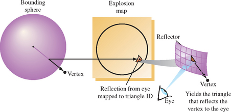
An explosion map can be thought of as a special environment map, encoding the volumes of space “owned” by the triangles in the reflector’s mesh. An explosion map stores reflection directions in a 2D image, in much the same way as OpenGL maps reflection directions to a sphere map. A unit vector (x, y, z)T is mapped into coordinates s, t within a circle inscribed in an explosion map with radius r as
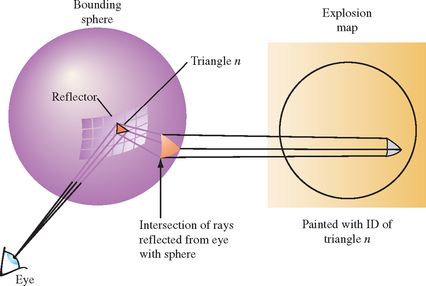
The reflection directions used in the mapping are not the actual reflection rays determined from the reflector vertex and the viewpoint. Rather, the reflection ray is intersected with a sphere and the normalized vector from the center of the sphere to the intersection point is used instead. There is a one-to-one mapping between reflection vectors from the convex reflector and intersection points on the sphere as long as the sphere encloses the reflector. Figure 17.9 shows a viewing vector V and a point P on the reflector that forms the reflection vector R as a reflection of V. The normalized direction vector D from the center of a sphere to the intersection of R with that sphere is inserted into the previous equation.
Once the reflection directions are mapped into 2D, an identification “color” for each triangle is rendered into the map using the mapped vertices for that triangle. This provides an exact mapping from any point on the sphere to the point that reflects that point to the viewpoint (see Figure 17.10). This identifier may be mapped using the color buffer, the depth buffer, or both. Applications need to verify the resolution available in the framebuffer and will likely need to disable dithering. If the color buffer is used, only the most significant bits of each component should be used. More details on using the color buffer to identify objects are discussed in Section 16.1.2.
Imagine a simplified scenario in which a vertex of a face to be reflected lies on the sphere. For this vertex on the sphere, the explosion map can be used to find a reflection plane the vertex is reflected across. The normalized vector pointing from the sphere center to the vertex is mapped into the explosion map to find a triangle ID. The mapped point formed from the vertex and the mapped triangle vertices are used to compute barycentric coordinates. These coordinates are used to interpolate a point and normal within the triangle that approximate a plane and normal on the curved reflector. The mapped vertex is reflected across this plane to form a virtual vertex. This process is illustrated in Figure 17.11.
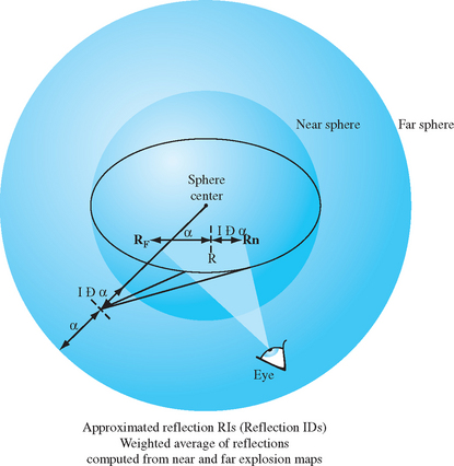
It may be impossible to find a single sphere that can be used to build an explosion map containing all vertices in the scene. To solve this problem, two separate explosion maps with two spheres are computed. One sphere tightly bounds the reflector object, while a larger sphere bounds the entire scene. The normalized vector from the center of each sphere to the vertex is used to look up the reflecting triangle in the associated explosion map. Although neither triangle may be correct, the reflected vertex can be positioned with reasonable accuracy by combining the results of both explosion maps to produce an approximation.
The results from the two maps are interpolated using a weight determined by the ratios of the distance from the surface of each sphere to the original vertex. Figure 17.12 shows how the virtual vertices determined from the explosion maps representing the near and far spheres are interpolated to find the final approximated reflected vertices.
Because the reflection directions from triangles in the reflector will not typically cover the entire explosion map, extension polygons are constructed that extend the reflection mappings to cover the map to its edges. These extension polygons can be thought of as extending the edges of profile triangles in the reflector into quadrilaterals that fully partition space. This ensures that all vertices in the original scene are reflected by some polygon.
If the reflector is a solid object, extension quadrilaterals may be formed from triangles in the reflector that have two vertex normals that face away from the viewer. If the reflector is convex, these triangles automatically lie on the boundary of the front-facing triangles in the reflector. The normals of each vertex are projected into the plane perpendicular to the viewer at that vertex, which guarantees that the reflection vector from the normals maps into the explosion map. This profile triangle is projected into the explosion map using these “adjusted” coordinates. The edge formed by the “adjusted” vertices is extended to a quadrilateral to cover the remaining explosion map area, which is rendered into the explosion map with the profile triangle’s identifier. It is enough to extend these vertices just beyond the boundary of the explosion map before rendering this quadrilateral. If the reflector is a surface that is not guaranteed to have back-facing polygons, it is necessary to extend the actual edges of the reflector until normals along the edge of the reflector fully span the space of angles in the x − y plane.
The technique described can be used for both convex and concave surfaces. Concave surfaces, however, have the additional complication that more than one triangle may “own” a given vertex. This prevents the algorithm from generating a good approximation to the reflection normal. Note, however, that the motion of such vertices will appear chaotic in an actual reflection, so arbitrarily choosing any one of the reflector triangles that owns the vertex will give acceptable results. A reflector with both convex and concave areas doesn’t have to be decomposed into separate areas. It is sufficient to structure the map so that each point on the explosion map is owned by only one triangle.
Trade-offs
The alternative to using object-space techniques for curved reflectors is environment mapping. Sphere or cube map texture can be generated at the center of the reflector, capturing the surrounding geometry, and a texgen function can be applied to the reflector to show the reflection. This alternative will work well when the reflecting geometry isn’t too close to the reflector, and when the curvature of the reflector isn’t too high, or when the reflection doesn’t have to be highly accurate. An object-space method that creates virtual reflected objects, such as the explosion map method, will work better for nearby objects and more highly curved reflectors. Note that the explosion map method itself is still an approximation: it uses a texture map image to find the proper triangle and compute the reflection point. Because of this, explosion maps can suffer from image-space sampling issues.
17.1.4 Interreflections
The reflection techniques described here can be extended to model interreflections between objects. An invocation of the technique is used for every reflection “bounce” between objects to be represented. In practice, the number of bounces must be limited to a small number (often less than four) in order to achieve acceptable performance.
The geometry-based techniques require some refinements before they can be used to model multiple interreflections. First, reflection transforms need to be concatenated to create multiple interreflection transforms. This is trivial for planar transforms; the OpenGL matrix stack can be used. Concatenating curved reflections is more involved, since the transform varies per-vertex. The most direct approach is to save the geometry generated at each reflection stage and then use it to represent the scene when computing the next level of reflection. Clipping multiple reflections so that they stay within the bounds of the reflectors becomes more complicated. The clipping method must be structured so that it can be applied repeatably at each reflection step. Improper clipping after the last interreflection can leave excess incorrect geometry in the image.
When clipping with a stencil, it is important to order the stencil operations so that the reflected scene images are masked directly by the stencil buffer as they are rendered. Render the reflections with the deepest recursion first. Concatenate the reflection transformations for each reflection polygon involved in an interreflection. The steps of this approach are outlined here.
2. Set the stencil operation to increment stencil values where pixels are rendered.
3. Render each reflector involved in the interreflection into the stencil buffer.
4. Set the stencil test to pass where the stencil value equals the number of reflections.
5. Apply planar reflection transformation overall, or apply curved reflection transformation per-vertex.
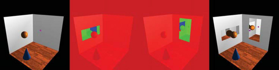
Figure 17.13 illustrates how the stencil buffer can segment the components of interreflecting mirrors. The leftmost panel shows a scene without mirrors. The next two panels show a scene reflected across two mirrors. The coloring illustrates how the scene is segmented by different stencil values—red shows no reflections, green one, and blue two. The rightmost panel shows the final scene with all reflections in place, clipped to the mirror boundaries by the stencil buffer.
As with ray tracing and radiosity techniques, there will be errors in the results stemming from the interreflections that aren’t modeled. If only two interreflections are modeled, for example, errors in the image will occur where three or more interreflections should have taken place. This error can be minimized through proper choice of an “initial color” for the reflectors. Reflectors should have an initial color applied to them before modeling reflections. Any part of the reflector that doesn’t show an interreflection will have this color after the technique has been applied. This is not an issue if the reflector is completely surrounded by objects, such as with indoor scenes, but this isn’t always the case. The choice of the initial color applied to reflectors in the scene can have an effect on the number of passes required. The initial reflection value will generally appear as a smaller part of the picture on each of the passes. One approach is to set the initial color to the average color of the scene. That way, errors in the interreflected view will be less noticeable.
When using the texture technique to apply the reflected scene onto the reflector, render with the deepest reflections first, as described previously. Applying the texture algorithm for multiple interreflections is simpler. The only operations required to produce an interreflection level are to apply the concatenated reflection transformations, copy the image to texture memory, and paint the reflection image to the reflector to create the intermediate scene as input for the next pass. This approach only works for planar reflectors, and doesn’t capture the geometry warping that occurs with curved ones. Accurate nonplanar interreflections require using distorted reflected geometry as input for intermediate reflections, as described previously. If high accuracy isn’t necessary, using environment mapping techniques to create the distorted reflections coming from curved objects makes it possible to produce multiple interreflections more simply.
Using environment mapping makes the texture technique the same for planar and nonplanar algorithms. At each interreflection step, the environment map for each object is updated with an image of the surrounding scene. This step is repeated for all reflectors in the scene. Each environment map will be updated to contain images with more interreflections until the desired number of reflections is achieved.
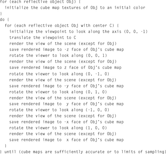
To illustrate this idea, consider an example in which cube maps are used to model the reflected surroundings “seen” by each reflective (and possibly curved) object in the scene. Begin by initializing the contents of the cube map textures owned by each of the reflective objects in the scene. As discussed previously, the proper choice of initial values can minimize error in the final image or alternatively, reduce the number of interreflectons needed to achieve acceptable results. For each interreflection “bounce,” render the scene, cube-mapping each reflective object with its texture. This rendering step is iterative, placing the viewpoint at the center of each object and looking out along each major axis. The resulting images are used to update the object’s cube map textures. The following pseudocode illustrates how this algorithm might be implemented.
Once the environment maps are sufficiently accurate, the scene is rerendered from the normal viewpoint, with each reflector textured with its environment map. Note that during the rendering of the scene other reflective objects must have their most recent texture applied. Automatically determining the number of interreflections to model can be tricky. The simplest technique is to iterate a certain number of times and assume the results will be good. More sophisticated approaches can look at the change in the sphere maps for a given pass, or compute the maximum possible change given the projected area of the reflective objects.
When using any of the reflection techniques, a number of shortcuts are possible. For example, in an interactive application with moving objects or a moving viewpoint it may be acceptable to use the reflection texture with the content from the previous frame. Having this sort of shortcut available is one of the advantages of the texture mapping technique. The downside of this approach is obvious: sampling errors. After some number of iterations, imperfect sampling of each image will result in noticeable artifacts. Artifacts can limit the number of interreflections that can be used in the scene. The degree of sampling error can be estimated by examining the amount of magnification and minification encountered when a texture image applied to one object is captured as a texture image during the rendering process.
Beyond sampling issues, the same environment map caveats also apply to interreflections. Nearby objects will not be accurately reflected, self-reflections on objects will be missing, and so on. Fortunately, visually acceptable results are still often possible; viewers do not often examine reflections very closely. It is usually adequate if the overall appearance “looks right.”
17.1.5 Imperfect Reflectors
The techniques described so far model perfect reflectors, which don’t exist in nature. Many objects, such as polished surfaces, reflect their surroundings and show a surface texture as well. Many are blurry, showing a reflected image that has a scattering component. The reflection techniques described previously can be extended to objects that show these effects.
Creating surfaces that show both a surface texture and a reflection is straightforward. A reflection pass and a surface texture pass can be implemented separately, and combined at some desired ratio with blending or multitexturing. When rendering a surface texture pass using reflected geometry, depth buffering should be considered. Adding a surface texture pass could inadvertently update the depth buffer and prevent the rendering of reflected geometry, which will appear “behind” the reflector. Proper ordering of the two passes, or rendering with depth buffer updating disabled, will solve the problem. If the reflection is captured in a surface texture, both images can be combined with a multipass alpha blend technique, or by using multitexturing. Two texture units can be used—one handling the reflection texture and the other handling the surface one.
Modeling a scattering reflector that creates “blurry” reflections can be done in a number of ways. Linear fogging can approximate the degradation in the reflection image that occurs with increasing distance from the reflector, but a nonlinear fogging technique (perhaps using a texture map and a texgen function perpendicular to the translucent surface) makes it possible to tune the fade-out of the reflected image.
Blurring can be more accurately simulated by applying multiple shearing transforms to reflected geometry as a function of its perpendicular distance to the reflective surface. Multiple shearing transforms are used to simulate scattering effects of the reflector. The multiple instances of the reflected geometry are blended, usually with different weighting factors. The shearing direction can be based on how the surface normal should be perturbed according to the reflected ray distribution. This distribution value can be obtained by sampling a BRDF. This technique is similar to the one used to generate depth-of-field effects, except that the blurring effect applied here is generally stronger. See Section 13.3 for details. Care must be taken to render enough samples to reduce visible error. Otherwise, reflected images tend to look like several overlaid images rather than a single blurry one. A high-resolution color buffer or the accumulation buffer may be used to combine several reflection images with greater color precision, allowing more images to be combined.
In discussing reflection techniques, one important alternative has been overlooked so far: ray tracing. Although it is usually implemented as a CPU-based technique without acceleration from the graphics hardware, ray tracing should not be discounted as a possible approach to modeling reflections. In cases where adequate performance can be achieved, and high-quality results are necessary, it may be worth considering ray tracing and Metropolis light transport (Veach, 1997) for providing reflections. The resulting application code may end up more readable and thus more maintainable.
Using geometric techniques to accurately implement curved reflectors and blurred reflections, along with culling techniques to improve performance, can lead to very complex code. For small reflectors, ray tracing may achieve sufficient performance with much less algorithmic complexity. Since ray tracing is well established, it is also possible to take advantage of existing ray-tracing code libraries. As CPUs increase in performance, and multiprocessor and hyperthreaded machines slowly become more prevalent, it may be the case that brute-force algorithms may provide acceptable performance in many cases without adding excessive complexity.
Ray tracing is well documented in the computer graphics literature. There are a number of ray-tracing survey articles and course materials available through SIGGRAPH, such as Hanrahan and Michell’s paper (Hanrahan, 1992), as well as a number of good texts (Glassner, 1989; Shirley, 2003) on the subject.
17.2 Refraction
Refraction is defined as the “change in the direction of travel as light passes from one medium to another” (Cutnell, 1989). The change in direction is caused by the difference in the speed of light between the two media. The refractivity of a material is characterized by the index of refraction of the material, or the ratio of the speed of light in the material to the speed of light in a vacuum (Cutnell, 1989). With OpenGL we can duplicate refraction effects using techniques similar to the ones used to model reflections.
17.2.1 Refraction Equation
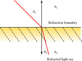
The direction of a light ray after it passes from one medium to another is computed from the direction of the incident ray, the normal of the surface at the intersection of the incident ray, and the indices of refraction of the two materials. The behavior is shown in Figure 17.14. The first medium through which the ray passes has an index of refraction n1, and the second has an index of refraction n2. The angle of incidence, θ1, is the angle between the incident ray and the surface normal. The refracted ray forms the angle θ2 with the normal. The incident and refracted rays are coplanar. The relationship between the angle of incidence and the angle of refraction is stated as Snell’s law (Cutnell, 1989):
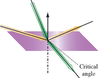
If n1 >n2 (light is passing from a more refractive material to a less refractive material), past some critical angle the incident ray will be bent so far that it will not cross the boundary. This phenomenon is known as total internal reflection, illustrated in Figure 17.15 (Cutnell, 1989).
Snell’s law, as it stands, is difficult to use with computer graphics. A version more useful for computation (Foley, 1994) produces a refraction vector R pointing away from the interface. It is derived from the eye vector U incident to the interface, a normal vector N, and n, the ratio of the two indexes of refraction, ![]() :
:
If precision must be sacrificed to improve performance, further simplifications can be made. One approach is to combine the terms scaling N, yielding
An absolute measurement of a material’s refractive properties can be computed by taking the ratio of its n against a reference material (usually a vacuum), producing a refractive index. Table 17.1 lists the refractive indices for some common materials.
Table 17.1
Indices of Refraction for Some Common Materials
| Material | Index |
| Vacuum | 1.00 |
| Air | ∼1.00 |
| Glass | 1.50 |
| Ice | 1.30 |
| Diamond | 2.42 |
| Water | 1.33 |
| Ruby | 1.77 |
| Emerald | 1.57 |
Refractions are more complex to compute than reflections. Computation of a refraction vector is more complex than the reflection vector calculation since the change in direction depends on the ratio of refractive indices between the two materials. Since refraction occurs with transparent objects, transparency issues (as discussed in Section 11.8) must also be considered. A physically accurate refraction model has to take into account the change in direction of the refraction vector as it enters and exits the object. Modeling an object to this level of precision usually requires using ray tracing. If an approximation to refraction is acceptable, however, refracted objects can be rendered with derivatives of reflection techniques.
For both planar and nonplanar reflectors, the basic approach is to compute an eye vector at one or more points on the refracting surface, and then use Snell’s law (or a simplification of it) to find refraction vectors. The refraction vectors are used as a guide for distorting the geometry to be refracted. As with reflectors, both object-space and image-space techniques are available.
17.2.2 Planar Refraction
Planar refraction can be modeled with a technique that computes a refraction vector at one point on the refracting surface and then moves the eye point to a perspective that roughly matches the refracted view through the surface (Diefenbach, 1997). For a given viewpoint, consider a perspective view of an object. In object space, rays can be drawn from the eye point through the vertices of the transparent objects in the scene. Locations pierced by a particular ray will all map to the same point on the screen in the final image. Objects with a higher index of refraction (the common case) will bend the rays toward the surface normal as the ray crosses the object’s boundary and passes into it.
This bending toward the normal will have two effects. Rays diverging from an eye point whose line of sight is perpendicular to the surface will be bent so that they diverge more slowly when they penetrate the refracting object. If the line of sight is not perpendicular to the refractor’s surface, the bending effect will cause the rays to be more perpendicular to the refractor’s surface after they penetrate it.
These two effects can be modeled by adjusting the eye position. Less divergent rays can be modeled by moving the eye point farther from the object. The bending of off-axis rays to directions more perpendicular to the object surface can be modeled by rotating the viewpoint about a point on the reflector so that the line of sight is more perpendicular to the refractor’s surface.
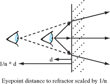
Computing the new eye point distance is straightforward. From Snell’s law, the change in direction crossing the refractive boundary, ![]() , is equal to the ratio of the two indices of refraction n. Considering the change of direction in a coordinate system aligned with the refractive boundary, n can be thought of as the ratio of vector components perpendicular to the normal for the unrefracted and refracted vectors. The same change in direction would be produced by scaling the distance of the viewpoint from the refractive boundary by
, is equal to the ratio of the two indices of refraction n. Considering the change of direction in a coordinate system aligned with the refractive boundary, n can be thought of as the ratio of vector components perpendicular to the normal for the unrefracted and refracted vectors. The same change in direction would be produced by scaling the distance of the viewpoint from the refractive boundary by ![]() , as shown in Figure 17.16.
, as shown in Figure 17.16.
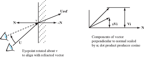
Rotating the viewpoint to a position more face-on to the refractive interface also uses n. Choosing a location on the refractive boundary, a vector U from the eye point to the refractor can be computed. The refracted vector components are obtained by scaling the components of the vector perpendicular to the interface normal by n. To produce the refracted view, the eye point is rotated so that it aligns with the refracted vector. The rotation that makes the original vector colinear with the refracted one using dot products to find the sine and cosine components of the rotation, as shown in Figure 17.17.
17.2.3 Texture Mapped Refraction
The viewpoint method, described previously, is a fast way of modeling refractions, but it has limited application. Only very simple objects can be modeled, such as a planar surface. A more robust technique, using texture mapping, can handle more complex boundaries. It it particularly useful for modeling a refractive surface described with a height field, such as a liquid surface.
The technique computes refractive rays and uses them to calculate the texture coordinates of a surface behind the refractive boundary. Every object that can be viewed through the refractive media must have a surface texture and a mapping for applying it to the surface. Instead of being applied to the geometry behind the refractive surface, texture is applied to the surface itself, showing a refracted view of what’s behind it. The refractive effect comes from careful choice of texture coordinates. Through ray casting, each vertex on the refracting surface is paired with a position on one of the objects behind it. This position is converted to a texture coordinate indexing the refracted object’s texture. The texture coordinate is then applied to the surface vertex.
The first step of the algorithm is to choose sample points that span the refractive surface. To ensure good results, they are usually regularly spaced from the perspective of the viewpoint. A surface of this type is commonly modeled with a triangle or quad mesh, so a straightforward approach is to just sample at each vertex of the mesh. Care should be taken to avoid undersampling; samples must capture a representative set of slopes on the liquid surface.
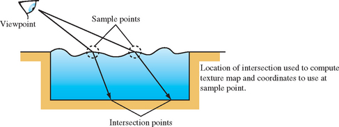
At each sample point the relative eye position and the indices of refraction are used to compute a refractive ray. This ray is cast until it intersects an object in the scene behind the refractive boundary. The position of the intersection is used to compute texture coordinates for the object that matches the intersection point. The coordinates are then applied to the vertex at the sample point. Besides setting the texture coordinates, the application must also note which surface was intersected, so that it can use that texture when rendering the surface near that vertex. The relationship among intersection position, sample point, and texture coordinates is shown in Figure 17.18.
The method works well where the geometry behind the refracting surface is very simple, so the intersection and texture coordinate computation are not difficult. An ideal application is a swimming pool. The geometry beneath the water surface is simple; finding ray intersections can be done using a parameterized clip algorithm. Rectangular geometry also makes it simple to compute texture coordinates from an intersection point.
It becomes more difficult when the geometry behind the refractor is complex, or the refracting surface is not generally planar. Efficiently casting the refractive rays can be difficult if they intersect multiple surfaces, or if there are many objects of irregular shape, complicating the task of associating an intersection point with an object. This issue can also make it difficult to compute a texture coordinate, even after the correct object is located.
Since this is an image-based technique, sampling issues also come into play. If the refractive surface is highly nonplanar, the intersections of the refracting rays can have widely varying spacing. If the textures of the intersected objects have insufficient resolution, closely spaced intersection points can result in regions with unrealistic, highly magnified textures. The opposite problem can also occur. Widely spaced intersection points will require mipmapped textures to avoid aliasing artifacts.
17.2.4 Environment Mapped Refraction
A more general texturing approach to refraction uses a grid of refraction sample points paired with an environment map. The map is used as a general lighting function that takes a 3D vector input. The approach is view dependent. The viewer chooses a set of sample locations on the front face of the refractive object. The most convenient choice of sampling locations is the refracting object’s vertex locations, assuming they provide adequate sampling resolution.
At each sample point on the refractor, the refraction equation is applied to find the refracted eye vector at that point. The x, y, and z components of the refracted vector are applied to the appropriate vertices by setting their s, t, and r texture components. If the object vertices are the sample locations, the texture coordinates can be directly applied to the sampled vertex. If the sample points don’t match the vertex locations, either new vertices are added or the grid of texture coordinates is interpolated to the appropriate vertices.
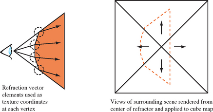
An environment texture that can take three input components, such as a cube (or dual-paraboloid) map, is created by embedding the viewpoint within the refractive object and then capturing six views of the surrounding scene, aligned with the coordinate system’s major axes. Texture coordinate generation is not necessary, since the application generates them directly. The texture coordinates index into the cube map, returning a color representing the portion of the scene visible in that direction. As the refractor is rendered, the texturing process interpolates the texture coordinates between vertices, painting a refracted view of the scene behind the refracting object over its surface, as shown in Figure 17.19.
The resulting refractive texture depends on the relative positions of the viewer, the refractive object, and to a lesser extent the surrounding objects in the scene. If the refracting object changes orientation relative to the viewer, new samples must be generated and the refraction vectors recomputed. If the refracting object or other objects in the scene change position significantly, the cube map will need to be regenerated.
As with other techniques that depend on environment mapping, the resulting refractive image will only be an approximation to the correct result. The location chosen to capture the cube map images will represent the view of each refraction vector over the surface of the image. Locations on the refractor farther from the cube map center point will have greater error. The amount of error, as with other environment mapping techniques, depends on how close other objects in the scene are to the refractor. The closer objects are to the refractor, the greater the “parallax” between the center of the cube map and locations on the refractor surface.
17.2.5 Modeling Multiple Refraction Boundaries
The process described so far only models a single transition between different refractive indices. In the general case, a refractive object will be transparent enough to show a distorted view of the objects behind the refractor, not just any visible structures or objects inside. To show the refracted view of objects behind the refractor, the refraction calculations must be extended to use two sample points, computing the light path as it goes into and out of the refractor.
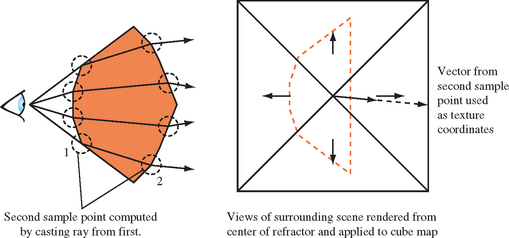
As with the single sample technique, a set of sample points are chosen and refraction vectors are computed. To model the entire refraction effect, a ray is cast from the sample point in the direction of the refraction vector. An intersection is found with the refractor, and a new refraction vector is found at that point, as shown in Figure 17.20. The second vector’s components are stored at texture coordinates at the first sample point’s location. The environment mapping operation is the same as with the first approach. In essence, the refraction vector at the sample point is more accurate, since it takes into account the refraction effect from entering and leaving the refractive object.
In both approaches, the refractor is ray traced at a low sampling resolution, and an environment map is used to interpolate the missing samples efficiently. This more elaborate approach suffers from the same issues as the single-sample one, with the additional problem of casting a ray and finding the second sample location efficiently. The approach can run into difficulties if parts of the refractor are concave, and the refracted ray can intersect more than one surface.
The double-sampling approach can also be applied to the viewpoint shifting approach described previously. The refraction equation is applied to the front surface, and then a ray is cast to find the intersection point with the back surface. The refraction equation is applied to the new sample point to find the refracted ray. As with the single-sample version of this approach, the viewpoint is rotated and shifted to approximate the refracted view. Since the entire refraction effect is simulated by changing the viewpoint, the results will only be satisfactory for very simple objects, and if only a refractive effect is required.
17.2.6 Clipping Refracted Objects
Clipping refracted geometry is identical to clipping reflected geometry. Clipping to the refracting surface is still necessary, since refracted geometry, if the refraction is severe enough, can cross the refractor’s surface. Clipping to the refractor’s boundaries can use the same stencil, clip plane, and texture techniques described for reflections. See Section 17.1.2 for details.
Refractions can also be made from curved surfaces. The same parametric approach can be used, applying the appropriate refraction equation. As with reflectors, the transformation lookup can be done with an extension of the explosion map technique described in Section 17.8. The map is created in the same way, using refraction vectors instead of reflection vectors to create the map. Light rays converge through some curved refractors and diverge through others. Refractors that exhibit both behaviors must be processed so there is only a single triangle owning any location on the explosion map.
Refractive surfaces can be imperfect, just as there are imperfect reflectors. The refractor can show a surface texture, or a reflection (often specular). The same techniques described in Section 17.1.5 can be applied to implement these effects.
The equivalent to blurry reflections—translucent refractors—can also be implemented. Objects viewed through a translucent surface become more difficult to see the further they are from the reflecting or transmitting surface, as a smaller percentage of unscattered light is transmitted to the viewer. To simulate this effect, fogging can be enabled, where fogging is zero at the translucent surface and increases as a linear function of distance from that surface. A more accurate representation can rendering multiple images with a divergent set of refraction vectors, and blend the results, as described in Section 17.1.5.
17.3 Creating Environment Maps
The basics of environment mapping were introduced in Section 5.4, with an emphasis on configuring OpenGL to texture using an environment map. This section completes the discussion by focusing on the creation of environment maps. Three types of environment maps are discussed: cube maps, sphere maps, and dual-paraboloid maps. Sphere maps have been supported since the first version of OpenGL, while cube map support is more recent, starting with OpenGL 1.3. Although not directly supported by OpenGL, dual-paraboloid mapping is supported through the reflection map texture coordinate generation functionality added to support cube mapping.
An important characteristic of an environment map is its sampling rate. An environment map is trying to solve the problem of projecting a spherical view of the surrounding environment onto one or more flat textures. All environment mapping algorithms do this imperfectly. The sampling rate—the amount of the spherical view a given environment mapped texel covers—varies across the texture surface. Ideally, the sampling rate doesn’t change much across the texture. When it does, the textured image quality will degrade in areas of poor sampling, or texture memory will have to be wasted by boosting texture resolution so that those regions are adequately sampled. The different environment mapping types have varying performance in this area, as discussed later.
The degree of sampling rate variation and limitations of the texture coordinate generation method can make a particular type of environment mapping view dependent or view independent. The latter condition is the desirable one because a view-independent environment mapping method can generate an environment that can be accurately used from any viewing direction. This reduces the need to regenerate texture maps as the viewpoint changes. However, it doesn’t eliminate the need for creating new texture maps dynamically. If the objects in the scene move significantly relative to each other, a new environment map must be created.
In this section, physical render-based, and ray-casting methods for creating each type of environment map textures are discussed. Issues relating to texture update rates for dynamic scenes are also covered. When choosing an environment map method, key considerations are the quality of the texture sampling, the difficulty in creating new textures, and its suitability as a basic building block for more advanced techniques.
17.3.1 Creating Environment Maps with Ray Casting
Because of its versatility, ray casting can be used to generate environment map texture images. Although computationally intensive, ray casting provides a great deal of control when creating a texture image. Ray-object interactions can be manipulated to create specific effects, and the number of rays cast can be controlled to provide a specific image quality level. Although useful for any type of environment map, ray casting is particularly useful when creating the distorted images required for sphere and dual-paraboloid maps.
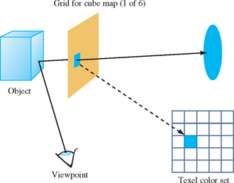
Ray casting an environment map image begins with a representation of the scene. In it are placed a viewpoint and grids representing texels on the environment map. The viewpoint and grid are positioned around the environment-mapped object. If the environment map is view dependent, the grid is oriented with respect to the viewer. Rays are cast from the viewpoint, through the grid squares and out into the surrounding scene. When a ray intersects an object in the scene, a color reflection ray value is computed, which is used to determine the color of a grid square and its corresponding texel (Figure 17.21). If the grid is planar, as is the case for cube maps, the ray-casting technique can be simplified to rendering images corresponding to the views through the cube faces, and transfering them to textures.
There are a number of different methods that can be applied when choosing rays to cast though the texel grid. The simplest is to cast a ray from the viewpoint through the center of each texel. The color computed by the ray-object intersection becomes the texel color. If higher quality is required, multiple rays can be cast through a single texel square. The rays can pass through the square in a regular grid, or jittered to avoid spatial aliasing artifacts. The resulting texel color in this case is a weighted sum of the colors determined by each ray. A beam-casting method can also be used. The viewpoint and the corners of the each texel square define a beam cast out into the scene. More elaborate ray-casting techniques are possible and are described in other ray tracing texts.
17.3.2 Creating Environment Maps with Texture Warping
Environment maps that use a distorted image, such as sphere maps and dual-paraboloid maps, can be created from six cube-map-style images using a warping approach. Six flat, textured, polygonal meshes called distortion meshes are used to distort the cube-map images. The images applied to the distortion meshes fit together, in a jigsaw puzzle fashion, to create the environment map under contruction. Each mesh has one of the cube map textures applied to it. The vertices on each mesh have positions and texture coordinates that warp its texture into a region of the environment map image being created. When all distortion maps are positioned and textured, they create a flat surface textured with an image of the desired environment map. The resulting geometry is rendered with an orthographic projection to capture it as a single texture image.
The difficult part of warping from cube map to another type of environment map is finding a mapping between the two. As part of its definition, each environment map has a function env() for mapping a vector (either a reflection vector or a normal) into a pair of texture coordinates: its general form is (s, t) = f(Vx, Vy, Vz). This function is used in concert with the cube-mapping function cube(), which also takes a vector (Vx, Vy, Vz) and maps it to a texture face and an (s, t) coordinate pair. The largest R component becomes the major axis, and determines the face. Once the major axis is found, the other two components of R become the unscaled s and t values, sc and tc. Table 17.2 shows which components become the unscaled s and t given a major axis ma. The correspondence between env() and cube() determines both the valid regions of the distortion grids and what texture coordinates should be assigned to their vertices.
To illustrate the relationship between env() and cube(), imagine creating a set of rays emanating from a single point. Each of the rays is evenly spaced from its neighbors by a fixed angle, and each has the same length. Considering these rays as vectors provides a regular sampling of every possible direction in 3D space. Using the cube() function, these rays can be segmented into six groups, segregated by the major axis they are aligned with. Each group of vectors corresponds to a cube map face.
If all texture coordinates generated by env() are transformed into 2D positions, a nonuniform flat mesh is created, corresponding to texture coordinates generated by env()’s environment mapping method. These vertices are paired with the texture coordinates generated by cube() from the same vectors. Not every vertex created by env() has a texture coordinate generated by cube(); the coordinates that don’t have cooresponding texture coordinates are deleted from the grid. The regions of the mesh are segmented, based on which face cube() generates for a particular vertex/vector. These regions are broken up into separate meshes, since each corresponds to a different 2D texture in the cube map, as shown in Figure 17.22.
When this process is completed, the resulting meshes are distortion grids. They provide a mapping between locations on each texture representing a cube-map face with locations on the environment map’s texture. The textured images on these grids fit together in a single plane. Each is textured with its corresponding cube map face texture, and rendered with an orthogonal projection perpendicular to the plane. The resulting image can be used as texture for the environment map method that uses env().
In practice, there are more direct methods for creating proper distortion grids to map env() = cube(). Distortion grids can be created by specifying vertex locations corresponding to locations on the target texture map, mapping from these locations to the corresponding target texture coordinates, then a (linear) mapping to the corresponding vector (env()−1), and then mapping to the cubemap coordinates (using cube()) will generate the texture coordinates for each vertex. The steps to R and back can be skipped if a direct mapping from the target’s texture coordinates to the cube-map’s can be found. Note that the creation of the grid is not a performance-critical step, so it doesn’t have to be optimal. Once the grid has been created, it can be used over and over, applying different cube map textures to create different target textures.
There are practical issues to deal with, such as choosing the proper number of vertices in each grid to get adequate sampling, and fitting the grids together so that they form a seamless image. Grid vertices can be distorted from a regular grid to improve how the images fit together, and the images can be clipped by using the geometry of the grids or by combining the separate images using blending. Although a single image is needed for sphere mapping, two must be created for dual-paraboloid maps. The directions of the vectors can be used to segement vertices into two separate groups of distortion grids.
Warping with a Cube Map
Instead of warping the equivalent of a cube-map texture onto the target texture, a real cube map can be used to create a sphere map or dual-paraboloid map directly. This approach isn’t as redundant as it may first appear. It can make sense, for example, if a sphere or dual-paraboloid map needs to be created only once and used statically in an application. The environment maps can be created on an implementation that supports cube mapping. The generated textures can then be used on an implementation that doesn’t. Such a scenario might arise if the application is being created for an embedded environment with limited graphics hardware. It’s also possible that an application may use a mixture of environment mapping techniques, using sphere mapping on objects that are less important in the scene to save texture memory, or to create simple effect, such as a specular highlight.
Creating an environment map image using cube-map texturing is simpler than the texture warping procedure outlined previously. First, a geometric representation of the environment map is needed: a sphere for a sphere map, and two paraboloid disks for the dual-paraboloid map. The vertices should have normal vectors, perpendicular to the surface.
The object is rendered with the cube map enabled. Texture coordinate generation is turned on, usually using GL_REFLECTION_MAP, although GL_NORMAL_MAP could also be used in some cases. The image of the rendered object is rendered with an orthographic projection, from a viewpoint corresponding to the texture image desired. Since sphere mapping is viewer dependent, the viewpoint should be chosen so that the proper cube-map surfaces are facing the viewer. Dual-paraboloid maps require two images, captured from opposing viewpoints. As with the ray tracing and warping method, the resulting images can be copied to texture memory and used as the appropriate environment map.
17.3.3 Cube Map Textures
Cube map textures, as the name implies, are six textures connected to create the faces of an axis-aligned cube, which operate as if they surround the object being environment mapped. Each texture image making up a cube face is the same size as the others, and all have square dimensions. Texture faces are normal 2D textures. They can have texture borders, and can be mipmapped.
Since the textures that use them are flat, square, and oriented in the environment perpendicular to the major axes, cube-map texture images are relatively easy to create. Captured images don’t need to be distorted before being used in a cube map. There is a difference in sampling rate across the texture surface, however. The best-case (center) to worst-case sampling (the four corners) rate has a ratio of about ![]() this is normally handled by choosing an adequate texture face resolution.
this is normally handled by choosing an adequate texture face resolution.
In OpenGL, each texture face is a separate texture target, with a name based on the major axis it is perpendicular to, as shown in Table 17.3. The second and third columns show the directions of increasing s and t for each face.
Table 17.3
Relationship Between Major Axis and s and t Coordinates
| target (major axis) | Sc | tc |
| GL_TEXTURE_CUBE_MAP_POSITIVE_X | −z | −y |
| GL_TEXTURE_CUBE_MAP_NEGATIVE_X | z | −y |
| GL TEXTURE CUBE MAP POSITIVE_Y | x | z |
| GL_TEXTURE_CUBE_MAP_NEGATIVE_Y | x | −z |
| GL_TEXTURE_CUBE_MAP_POSITIVE_Z | x | −y |
| GL_TEXTURE_CUBE_MAP_NEGATIVE_Z | −x | −y |
Note that the orientation of the texture coordinates of each face are counter-intuitive. The origin of each texture appears to be “upper left” when viewed from the outside of the cube. Although not consistent with sphere maps or 2D texture maps, in practice the difference is easy to handle by flipping the coordinates when capturing the image, flipping an existing image before loading the texture, or by modifying texture coordinates when using the mipmap.
Cube maps of a physical scene can be created by capturing six images from a central point, each camera view aligned with a different major axis. The field of view must be wide enough to image an entire face of a cube, almost 110 degrees if a circular image is captured. The camera can be oriented to create an image with the correct s and t axes directly, or the images can be oriented by inverting the pixels along the x and y axes as necessary.
Synthetic cube-map images can be created very easily. A cube center is chosen, preferably close to the “center” of the object to be environment mapped. A perspective projection with a 90-degree field of view is configured, and six views from the cube center, oriented along the six major axes are used to capture texture images.
The perspective views are configured using standard transform techniques. The glFrustum command is a good choice for loading the projection matrix, since it is easy to set up a frustum with edges of the proper slopes. A near plane distance should be chosen so that the textured object itself is not visible in the frustum. The far plane distance should be great enough to take in all surrounding objects of interest. Keep in mind the depth resolution issues discussed in Section 2.8. The left, right, bottom, and top values should all be the same magnitude as the near value, to get the slopes correct.
Once the projection matrix is configured, the modelview transform can be set with the gluLookAt command. The eye position should be at the center of the cube map. The center of interest should be displaced from the viewpoint along the major axis for the face texture being created. The modelview transform will need to change for each view, but the projection matrix can be held constant. The up direction can be chosen, along with swapping of left/right and/or bottom/top glFrustum parameters to align with the cube map s and t axes, to create an image with the proper texture orientation.
The following pseudocode fragment illustrates this method for rendering cube-map texture images. For clarity, it only renders a single face, but can easily be modified to loop over all six faces. Note that all six cube-map texture target enumerations have contiguous values. If the faces are rendered in the same order as the enumeration, the target can be chosen with a “GL_TEXTURE_CUBE_MAP_POSITIVE_Z + face”-style expression.
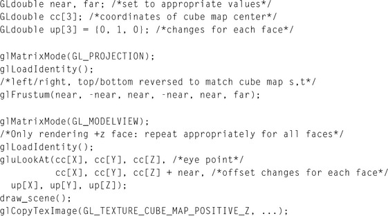
Note that the glFrustum command has its left, right, bottom, and top parameters reversed so that the resulting image can be used directly as a texture. The glCopyTexImage command can be used to transfer the rendered image directly into a texture map.
Two important quality issues should be considered when creating cube maps: texture sampling resolution and texture borders. Since the spatial sampling of each texel varies as a function of its distance from the center of the texture map, texture resolution should be chosen carefully. A larger texture can compensate for poorer sampling at the corners at the cost of more texture memory. The texture image itself can be sampled and nonuniformly filtered to avoid aliasing artifacts. If the cube-map texture will be minified, each texture face can be a mipmap, improving filtering at the cost of using more texture memory. Mipmapping is especially useful if the polygons that are environment mapped are small, and have normals that change direction abruptly from vertex to vertex.
Texture borders must be handled carefully to avoid visual artifacts at the seams of the cube map. The OpenGL specification doesn’t specify exactly how a face is chosen for a vector that points at an edge or a corner; the application shouldn’t make assumptions based on the behavior of a particular implementation. If textures with linear filtering are used without borders, setting the wrap mode to GL_CLAMP_TO_EDGE will produce the best quality. Even better edge quality results from using linear filtering with texture borders. The border for each edge should be obtained from the strip of edge texels on the adjacent face.
Loading border texels can be done as a postprocessing step, or the frustum can be adjusted to capture the border pixels directly. The mathematics for computing the proper frustum are straightforward. The cube-map frustum is widened so that the outer border of pixels in the captured image will match the edge pixels of the adjacent views. Given a texture resolution res—and assuming that the glFrustum call is using the same value len for the magnitude of the left, right, top, and bottom parameters (usually equal to near)—the following equation computes a new length parameter newlen:
In practice, simply using a one-texel-wide strip of texels from the adjacent faces of the borders will yield acceptable accuracy.
Border values can also be used with mipmapped cube-map faces. As before, the border texels should match the edge texels of the adjacent face, but this time the process should be repeated for each mipmap level. Adjusting the camera view to capture border textures isn’t always desirable. The more straightforward approach is to copy texels from adjacent texture faces to populate a texture border. If high accuracy is required, the area of each border texel can be projected onto the adjacent texture image and used as a guide to create a weighted sum of texel colors.
Cube-Map Ray Casting
The general ray-casting approach discussed in Section 17.3.1 can be easily applied to cube maps. Rays are cast from the center of the cube, through texel grids positioned as the six faces of the cube map, creating images for each face. The pixels for each image are computed by mapping a grid onto the cube face, corresponding to the desired texture resolution and then casting a ray from the center of the cube through each grid square out into the geometry of the surrounding scene. A pseudocode fragment illustrating the approach follows.
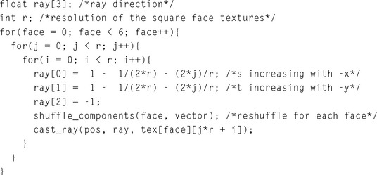
The cast_ray() function shoots a ray into the scene from pos, in the direction of ray, returning a color value based on what the ray intersects. The shuffle_components() function reorders the vertices, changing the direction of the vector for a given cube face.
17.3.4 Sphere Map Textures
A sphere map is a single 2D texture map containing a special image. The image is circular, centered on the texture, and shows a highly distorted view of the surrounding scene from a particular direction. The image can be described as the reflection of the surrounding environment off a perfectly reflecting unit sphere. This distorted image makes the sampling highly nonlinear, ranging from a one-to-one mapping at the center of the texture to a singularity around the circumference of the circular image.
If the viewpoint doesn’t move, the poor sampling regions will map to the silhouettes of the environment-mapped objects, and are not very noticeable. Because of this poor mapping near the circumference, sphere mapping is view dependent. Using a sphere map with a view direction or position significantly different from the one used to make it will move the poorly sampled texels into more prominent positions on the sphere-mapped objects, degrading image quality. Around the edge of the circular image is a singularity. Many texture map positions map to the same generated texture coordinate. If the viewer’s position diverges significantly from the view direction used to create the sphere map, this singularity can become visible on the sphere map object, showing up as a point-like imperfection on the surface.
There are two common methods used to create a sphere map of the physical world. One approach is to use a spherical object to reflect the surroundings. A photograph of the sphere is taken, and the resulting image is trimmed to the boundaries of the sphere, and then used as a texture. The difficulty with this, or any other physical method, is that the image represents a view of the entire surroundings. In this method, an image of the camera will be captured along with the surroundings.
Another approach uses a fish-eye lens to approximate sphere mapping. Although no camera image will be captured, no fish-eye lens can provide the 360-degree field of view required for a proper sphere map image.
Sphere Map Ray Casting
When a synthetic scene needs to be captured as a high-quality sphere map, the general ray-casting approach discussed in Section 17.3.1 can be used to create one. Consider the environment map image within the texture to be a unit circle. For each point (s, t) in the unit circle, a point P on the sphere can be computed:
Since it is a unit sphere, the normal at P is equal to P. Given the vector V toward the eye point, the reflected vector R is
In eye space, the eye point is at the origin, looking down the negative z axis, so V is a constant vector with value (0, 0, 1). Equation 17.1 reduces to
Combining the previous equations produces equations that map from (s, t) locations on the sphere map to R:
Given the reflection vector equation, rays can be cast from the center of the object location. The rays are cast in every direction; the density of the rays is influenced by the different sampling rates of a sphere map. The reflection vector equation can be used to map the ray’s color to a specific texel in the cube map. Since ray casting is expensive, an optimization of this approach is to only cast rays that correspond to a valid texel on the sphere map. The following pseudocode fragment illustrates the technique.

To minimize computational overhead, the code fragment uses the first two equations to produce a normal, and then a reflection vector, rather than compute the reflection vector directly. The cast_ray() function performs the ray/environment intersection given the starting point and the direction of the ray. Using the ray, it computes the color and puts the results into its third parameter (the location of the appropriate texel in the texture map).
The ray-casting technique can be used to create a texture based on the synthetic surroundings, or it can be used as a mapping function to convert a set of six cube map images into a sphere map. This approach is useful because it provides a straightforward method for mapping cube faces correctly onto the highly nonlinear sphere map image. The six images are overlayed on six faces of a cube centered around the sphere. The images represent what a camera with a 90-degree field of view and a focal point at the center of the square would see in the given direction. The cast rays intersect the cube’s image pixels to provide the sphere map texel values.
Sphere Map Warping
The texture warping approach discussed in Section 17.3.2 can be used to create sphere maps from six cube-map-style images. OpenGL’s texture mapping capabilities are used to distort the images and apply them to the proper regions on the sphere map. Unlike a ray-casting approach, the texture warping approach can be accelerated by graphics hardware. Depending on the technique, creating the distortion meshes may require a way to go from reflection vectors back into locations on the sphere map. The following equations perform this mapping.
Figure 17.23 shows the relationship of the distortion meshes for each cube face view to the entire sphere map mesh. The finer the tessellation of the mesh the better the warping. In practice, however, the mesh does not have to be extremely fine in order to construct a usable sphere map.
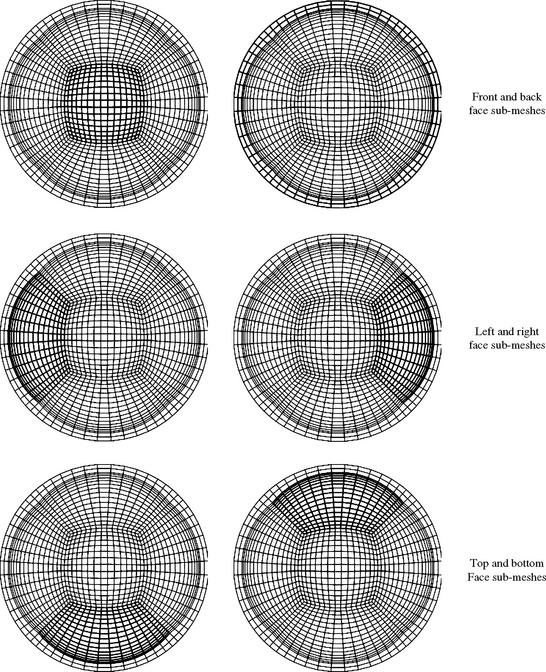
The distortion mesh for the back face of the cube must be handled in a special way. It is not a simple warped rectangular patch but a mesh in the shape of a ring. It can be visualized as the back cube view face pulled inside-out to the front. In a sphere map, the center of the back cube view face becomes a singularity around the circular edge of the sphere map. The easiest way to render the back face mesh is as four pieces. The construction of these meshes is aided by the reverse mapping equations. Using separate meshes makes it possible to apply the highly nonlinear transformation needed to make a cube map, but it leads to another problem. Combining meshes representing the six cube faces will result in a sphere with polygonal edges. To avoid this problem, a narrow “extender” mesh can be added, extending out from the circle’s edge. This ensures that the entire circular sphere map region is rendered.
Although the sphere map should be updated for every change in view, the meshes themselves are static for a given tessellation. They can be computed once and rerendered to extract a different view from the cube map. Precomputing the meshes helps reduce the overhead for repeated warping of cube face views into sphere map textures.
When the meshes are rendered, the sphere map image is complete. The final step is to copy it into a texture using glCopyTexImage2D.
17.3.5 Dual-paraboloid Maps
Dual-paraboloid mapping provides an environment mapping method between a sphere map—using a single image to represent the entire surrounding scene—and a cube map, which uses six faces, each capturing a 90-degree field of view. Dual paraboloid mapping uses two images, each representing half of the surroundings. Consider two parabolic reflectors face to face, perpendicular to the z axis. The convex back of each reflector reflects a 180-degree field of view. The circular images from the reflectors become two texture maps. One texture represents the “front” of the environment, capturing all of the reflection vectors with a nonnegative z component. The second captures all reflections with a z component less than or equal to zero. Both maps share reflections with a z component of zero.
Dual-paraboloid maps, unlike sphere maps, have good sampling characteristics, maintaining a 4-to-1 sampling ratio from the center to the edge of the map. It provides the best environment map sampling ratio, exceeding even cube maps. Because of this, and because dual-paraboloid maps use a three-component vector for texture lookup, dual-paraboloid maps are view independent. The techniques for creating dual-paraboloid maps are similar to those used for sphere maps. Because of the better sampling ratio and lack of singularities, high-quality dual-paraboloid maps are also easier to produce.
As with sphere mapping, a dual-paraboloid texture image can be captured physically. A parabolic reflector can be positioned within a scene, and using a camera along its axis an image captured of the reflector’s convex face. The process is repeated, with the reflector and camera rotated 180 degrees to capture an image of the convex face reflecting the view from the other side. As with sphere maps, the problem with using an actual reflector is that the camera will be in the resulting image.
A fish-eye lens approach can also be used. Since only a 180° field of view is required, a fish-eye lens can create a reasonable dual-paraboloid map, although the view distortion may not exactly match a parabolic reflector.
Dual-paraboloid Map Ray Casting
A ray-casting approach, as described in Section 17.3.1, can be used to create dual-paraboloid maps. The paraboloid surface can be assumed to cover a unit circle. A paraboloid for reflection vectors with a positive Rz component, centered around the z axis, has a parametric representation of
Taking the gradient, the normal at (s, t) is
As with sphere maps, the eye vector V simplifies in eye space to the constant vector (0, 0, 1). The reflection vector reduces to
Combining the normal and reflection equations produces two equations: one for the front side paraboloid and one for the back. These represent the reflection vector as a function of surface parameters on the paraboloid surfaces.
Given the reflection vector equation, rays can be cast from the location where the environment-mapped object will be rendered. The rays are cast in the direction specified by the reflection vector equations that match up with valid texel locations. Note that the rays cast will be segmented into two groups: those that update texels on the front-facing paraboloid map and those for the back-facing one. The following pseudocode fragment illustrates the technique.
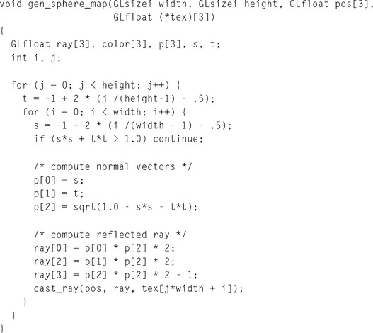
To minimize computational overhead, the code fragment uses the first two equations to produce a normal, then a reflection vector, rather than computing the reflection vector directly. The cast_ray() function performs the ray/environment intersection, given the starting point and the direction of the ray. Using the ray, it computes the color and puts the results into its third parameter (the location of the appropriate texel in the texture map).
Dual-paraboloid Map Warping
The texture warping approach discussed in Section 17.3.2 can be used to create dual-paraboloid maps from six cube-map-style images. OpenGL’s texture mapping capabilities are used to distort the images and apply them to the proper regions on the paraboloid maps. The texture warping approach can be accelerated. Creating the distortion meshes requires a way to go from reflection vectors back into locations on the paraboloid map. The following equations perform this mapping.
Figure 17.24 shows the relationship of the submesh for each cube face view to the dual-paraboloid-map mesh. The finer the tessellation of the mesh the better the warping, although usable paraboloid maps can be created with relatively coarse meshes, even coarser than sphere maps, since dual paraboloid maps don’t require strong warping of the image. Figure 17.24 shows how cube-map faces are arranged within the two dual-paraboloid map texture images, and Figure 17.25 shows the meshes required to do the warping.
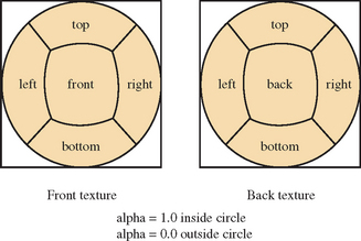
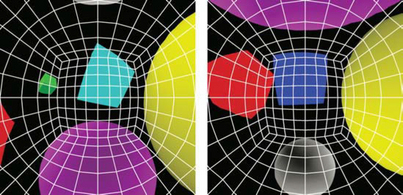
17.3.6 Updating Environment Maps Dynamically
Once the details necessary to create environment maps are understood, the next question is when to create or update them. The answer depends on the environment map type, the performance requirements of the application, and the required quality level.
Any type of environment map will need updating if the positional relationship between objects changes significantly. If some inaccuracy is acceptable, metrics can be created that can defer an update if the only objects that moved are small and distant enough from the reflecting object that their motion will not be noticeable in the reflection. These types of objects will affect only a small amount of surface on the reflecting objects. Other considerations, such as the contrast of the objects and whether they are visible from the reflector, can also be used to optimize environment map updates.
Sphere maps require the highest update overhead. They are the most difficult to create, because of their high distortion and singularities. Because they are so view dependent, sphere maps may require updates even if the objects in the scene don’t change position. If the view position or direction changes significantly, and the quality of the reflection is important in the application, the sphere map needs to be updated, for the reasons discussed in Section 17.3.4.
Dual-paraboloid maps are view independent, so view changes don’t require updating. Although they don’t have singularities, their creation still requires ray-casting or image warping techniques, so there is a higher overhead cost incurred when creating them. They do have the best sampling ratio, however, and so can be more efficient users of texture memory than cube maps.
Cube maps are the easiest to update. Six view face images, the starting point for sphere and dual-paraboloid maps, can be used directly by cube maps. Being view independent, they also don’t require updating when the viewer position changes.
17.4 Shadows
Shadows are an important method for adding realism to a scene. There are a number of trade-offs possible when rendering a scene with shadows (Woo, 1990). As with lighting, there are increasing levels of realism possible, paid for with decreasing levels of rendering performance.
Physically, shadows are composed of two parts: the umbra and the penumbra. The umbra is the area of a shadowed object that is not visible from any part of the light source. The penumbra is the area of a shadowed object that can receive some, but not all, of the light. A point source light has no penumbra, since no part of a shadowed object can receive only part of the light.
Penumbrae form a transition region between the umbra and the lighted parts of the object. The brightness across their surface varies as a function of the geometry of the light source and the shadowing object. In general, shadows usually create high-contrast edges, so they are more unforgiving with aliasing artifacts and other rendering errors.
Although OpenGL does not support shadows directly, it can be used to implement them a number of ways. The methods vary in their difficulty to implement, their performance, and the quality of their results. All three of these qualities vary as a function of two parameters: the complexity of the shadowing object and the complexity of the scene that is being shadowed.
17.4.1 Projective Shadows
A shadowing technique that is easy to implement is projective shadows. They can be created using projection transforms (Tessman, 1989; Blinn, 1988) to create a shadow as a distinct geometric object. A shadowing object is projected onto the plane of the shadowed surface and then rendered as a separate primitive. Computing the shadow involves applying an orthographic or perspective projection matrix to the modelview transform, and then rendering the projected object in the desired shadow color. Figure 17.26 illustrates the technique. A brown sphere is flattened and placed on the shadowed surface by redrawing it with an additional transform. Note that the color of the “shadow” is the same as the original object. The following is an outline of the steps needed to render an object that has a shadow cast from a directional light on the y-axis down onto the x, z plane.
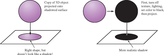
1. Render the scene, including the shadowing object.
2. Set the modelview matrix to identity, and then apply a projection transform such as glScalef with arguments 1.f, 0.f, 1.f.
3. Apply the other transformation commands necessary to position and orient the shadowing object.
4. Set the OpenGL state necessary to create the correct shadow color.
In the final step, the shadowing object is rendered a second time, flattened by the modelview transform into a shadow. This simple example can be expanded by applying additional transforms before the glScalef command to position the shadow onto the appropriate flat object. The direction of the light source can be altered by applying a shear transform after the glScalef call. This technique is not limited to directional light sources. A point source can be represented by adding a perspective transform to the sequence.
Shadowing with this technique is similar to decaling a polygon with another coplanar one. In both cases, depth buffer aliasing must be taken into account. To avoid aliasing problems, the shadow can be slightly offset from the base polygon using polygon offset, the depth test can be disabled, or the stencil buffer can be used to ensure correct shadow decaling. The best approach is depth buffering with polygon offset. Depth buffering will minimize the amount of clipping required. Depth buffer aliasing is discussed in more detail in Section 6.1.2 and Section 16.8.
Although an arbitrary shadow can be created from a sequence of transforms, it is often easier to construct a single-projection matrix directly. The following function takes an arbitrary plane, defined by the plane equation Ax + By + Cz + D = 0, and a light position in homogeneous coordinates. If the light is directional, the w value is set to 0. The function concatenates the shadow matrix with the current one.
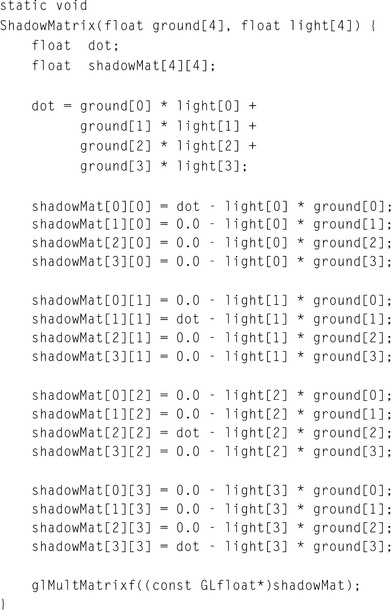
Projective Shadow Trade-offs
Although fast and simple to implement, the projective shadow technique is limited in a number of ways. First, it is difficult to shadow onto anything other than a flat surface. Although projecting onto a polygonal surfaces is possible (by carefully casting the shadow onto the plane of each polygon face) the results have to be clipped to each polygon’s boundaries. For some geometries, depth buffering will do the clipping automatically. Casting a shadow to the corner of a room composed of just a few perpendicular polygons is feasible with this method. Clipping to an arbitrary polgyonal surface being shadowed is much more difficult, and the technique becomes problematic if the shadowed object is image based (such as an object clipped by stenciling).
The other problem with projection shadows is controlling the shadow’s appearance. Since the shadow is a flattened version of the shadowing object, not the polygon being shadowed, there are limits to how well the shadow’s color can be controlled. The normals have been squashed by the projection operation, so properly lighting the shadow is impossible. A shadowed polygon with changing colors (such as a textured floor) won’t shadow correctly either, since the shadow is a copy of the shadowing object and must use its vertex information.
17.4.2 Shadow Volumes
This technique sheaths the shadow regions cast by shadowing objects with polygons, creating polygon objects called shadow volumes (see Figure 17.27). These volumes never update the color buffer directly. Instead, they are rendered in order to update the stencil buffer. The stencil values, in turn, are used to find the intersections between the polygons in the scene and the shadow volume surfaces (Crow, 1981; Bergeron, 1986; Heidmann, 1991).
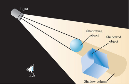
A shadow volume is constructed from the rays cast from the light source that intersect the vertices of the shadowing object. The rays continue past the vertices, through the geometery of the scene, and out of view. Defined in this way, the shadow volumes are semi-infinite pyramids, but they don’t have to be used that way. The technique works even if the base of the shadow volume is truncated as long as the truncation happens beyond any object that might be in the volume. The same truncation and capping can be applied to shadow volumes that pierce the front clipping plane as they go out of view. The truncation creates a polygonal object, whose interior volume contains shadowed objects or parts of shadowed objects. The polygons of the shadow volume should be defined so that their front faces point out from the shadow volume itself, so that they can be front-and back-face culled consistently.
The stencil buffer is used to compute which parts of the objects in the scene are enclosed in each shadow volume object. It uses a volumetric version of polygon rendering techniques. Either an even/odd or a non-zero winding rule can be used. Since the non-zero technique is more robust, the rest of the discussion will focus on this approach. Conceptually, the approach can be thought of as a 3D version of in/out testing. Rays are cast from the eye point into the scene; each ray is positioned to represent a pixel in the framebuffer. For each pixel, the stencil buffer is incremented every time its ray crosses into a shadow object, and decremented every time it leaves it. The ray stops when it encounters a visible object. As a result, the stencil buffer marks the objects in the scene with a value indicating whether the object is inside or outside a shadow volume. Since this is done on a per-pixel basis, an object can be partially inside a shadow volume and still be marked correctly.
The shadow volume method doesn’t actually cast rays through pixel positions into the shadow volumes and objects in the scene. Instead, it uses the depth buffer test to find what parts of the front and back faces of shadow volumes are visible from the viewpoint. In its simplest form, the entire scene is rendered, but only the depth buffer is updated. Then the shadow volumes are drawn. Before drawing the volume geometry, the color and depth buffers are configured so that neither can be updated but depth testing is still enabled. This means that only the visible parts of the shadow volumes can be rendered.
The volumes are drawn in two steps; the back-facing polygons of the shadow volume are drawn separately from the front. If the shadow volume geometry is constructed correctly, the back-facing polygons are the “back” of the shadow volume (i.e., farther from the viewer). When the back-facing geometry is drawn, the stencil buffer is incremented. Similarly, when the front-facing polygons of the shadow volumes are drawn the stencil buffer is set to decrement. Controlling whether the front-facing or back-face polygons are drawn is done with OpenGL’s culling feature. The resulting stencil values can be used to segment the scene into regions inside and outside the shadow volumes.
To understand how this technique works, consider the three basic scenarios possible when the shadow volumes are drawn. The result depends on the interaction of the shadow geometry with the current content of the depth buffer (which contains the depth values of the scene geometry). The results are evaluated on a pixel-by-pixel basis. The first scenario is that both the front and back of a shadow buffer are visible (i.e., all geometry at a given pixel is behind the shadow volume). In that case, the increments and decrements of the stencil buffer will cancel out, leaving the stencil buffer unchanged. The stencil buffer is also unchanged if the shadow volume is completely invisible (i.e., some geometry at a given pixel is in front of the shadow volume). In this case, the stencil buffer will be neither incremented or decremented. The final scenario occurs when geometry obscures the back surface of the shadow volume, but not the front. In this case, the stencil test will only pass on the front of the shadow volume, and the stencil value will be changed.
When the process is completed, pixels in the scene with non-zero stencil values identify the parts of an object in shadow. Stencil values of zero mean there was no geometry, or the geometry was completely in front of or behind the shadow volume.
Since the shadow volume shape is determined by the vertices of the shadowing object, shadow volumes can become arbitrarily complex. One consequence is that the order of stencil increments and decrements can’t be guaranteed, so a stencil value could be decremented below zero. OpenGL 1.4 added wrapping versions of the stencil increment and decrement operations that are robust to temporary overflows. However, older versions of OpenGL will need a modified version of the algorithm. This problem can be minimized by ordering the front- and back-facing shadow polygons to ensure that the stencil value will neither overflow nor underflow.
Another issue with counting is the position of the eye with respect to the shadow volume. If the eye is inside a shadow volume, the count of objects outside the shadow volume will be −1, not zero. This problem is discussed in more detail in Section 17.4. One solution to this problem is to add a capping polygon to complete the shadow volume where it is clipped by the front clipping plane, but this approach can be difficult to implement in a way that handles all clipping cases.
A pixel-based approach, described by a number of developers, (Carmack, 2000; Lengyel, 2002; Kilgard, 2002), changes the sense of the stencil test. Instead of incrementing the back faces of the shadow volumes when the depth test passes, the value is incremented only if the depth test fails. In the same way, the stencil value is only decremented where the front-facing polygons fail the depth test. Areas are in shadow where the stencil buffer values are non-zero. The stencil buffer is incremented where an object pierces the back face of a stencil volume, and decremented where they don’t pierce the front face. If the front face of the shadow volume is clipped away by the near clip plane, the stencil buffer is not decremented and the objects piercing the back face are marked as being in shadow. With this method, the stencil buffer takes into account pixels where the front face is clipped away (i.e., the viewer is in the shadow volume).
This approach doesn’t handle the case where the shadow volume is clipped away by the far clip plane. Although this scenario is not as common as the front clip plane case, it can be handled by capping the shadow volume to the far clip plane with extra geometry, or by extruding points “to infinity” by modifying the perspective transform. Modifying the transform is straightforward: two of the matrix elements of the standard glFrustum equation are modified, the ones using the far plane distance, f. The equations are evaluated with f at infinity, as shown here.
Taking f to infinity can lead to problems if the clip-space z value is greater than zero. A small epsilon value ε can be added:
Segmenting the Scene
The following outlines the shadow volume technique. Creating and rendering geometry extending from light sources and occluders, with the side effect of updating the stencil buffer, can be used to create shadows in a scene.
The simplest example is a scene with a single point-light source and a single occluder. The occluder casts a shadow volume, which is used to update the stencil buffer. The buffer contains non-zero values for objects in shadow, and zero values elsewhere. To create shadows, the depth buffer is cleared, and the entire scene is rendered with lighting disabled. The depth buffer is cleared again. The stencil buffer is then configured to only allow color and depth buffer updates where the stencil is zero. The entire scene is rendered again, this time with lighting enabled.
In essence, the entire scene is first drawn with the lights off, then with the lights on. The stencil buffer prevents shadowed areas from being overdrawn. The approach is broken out into more detailed steps shown here.
2. Enable color and depth buffers for writing and enable depth testing.
3. Set attributes for drawing in shadow and turn light sources off.
4. Render the entire scene (first time).
5. Compute the shadow volume surface polygons.
6. Disable color and depth buffer updates and enable depth testing.
8. Set stencil function to “always pass.”
9. Set stencil operations to increment when depth test fails.
10. Enable front-face culling.
11. Render shadow volume polygons.
12. Set stencil operations to decrement when depth test fails.
14. Render shadow volume polygons.
16. Set stencil function to test for equality to 0.
A complex object can generate a lot of shadow volume geometry. For complicated shadowing objects, a useful optimization is to find the object’s silhouette vertices, and just use them for creating the shadow volume. The silhouette vertices can be found by looking for any polygon edges that either (1) surround a shadowing object composed of a single polygon or (2) are shared by two polygons, one facing toward the light source and one facing away. The direction a polygon is facing can be found by taking the inner product of the polygon’s facet normal with the direction of the light source, or by a combination of selection and front- and back-face culling.
Multiple Light Sources
The shadow volume algorithm can be simply extended to handle multiple light sources. For each light source, repeat the second pass of the algorithm, clearing the stencil buffer to zero, computing the shadow volume polygons, and then rendering them to update the stencil buffer. Instead of replacing the pixel values of the unshadowed scenes, choose the appropriate blending function and add that light’s contribution to the scene for each light. If more color accuracy is desired, use the accumulation buffer.
This method can also be used to create soft shadows. Jitter the light source, choosing points that sample the light’s surface, and repeat the steps used to shadow multiple light sources.
Light Volumes
Light volumes are analogous to shadow volumes; their interpretation is simply reversed. Lighting is applied only within the volume, instead of outside it. This technique is useful for generating spotlight-type effects, especially if the light shape is complex. A complex light shape can result if the light source is partially blocked by multiple objects.
Incrementally Updating Shadow Volumes
Since computing shadow polygons is the most difficult part of the shadow volume technique, it’s useful to consider ways to reuse an existing volume whenever possible. One technique is useful for shadow or light volumes that are reflected in one or more planar surfaces. Instead of generating a new volume for each reflection, the original volume is transformed to match the light’s virtual position. The virtual position is where the light appears to be in the reflecting surface. The same reflection transform that moves the light from its actual position to the virtual one can be applied to the volume geometry.
Another technique is useful when the light or shadowing object moves only incrementally from frame to frame. As the light source moves, only the base of the volume (the part of the volume not attached to the light or shadowing object) requires updating. The change in vertex positions tracks the change in light position as a function of the ratio between the light-to-shadowing-object distance and the shadowing-object-to-base distance. A similar argument can be made when the shadowing object moves incrementally. In this case, some of the volume vertices move with the object (since it is attached to it). The base can be calculated using similar triangles. If either the light or shadowing object are moving linearly for multiple frames, a simplified equation can be generated for volume updates.
If the light source is being jittered to generate soft shadows, only the volume vertices attached to the shadowing object need to be updated. The base of the shadow volume can be left unchanged. Since the jitter movement is a constrained translation, updating these vertices only involves adding a constant jitter vector to each of them.
Shadow Volume Trade-offs
Shadow volumes can be very fast to compute when the shadowing object is simple. Difficulties occur when the shadowing object has a complex shape, making it expensive to compute the volume geometry. Ideally, the shadow volume should be generated from the vertices along the silhouette of the object, as seen from the light. This is not a trivial problem for a complex shadowing object.
In pathological cases, the shape of the shadow volume may cause a stencil value underflow. If the OpenGL implementation supports wrapping stencil increment and decrement,1 it can be used to avoid the problem. Otherwise, the zero stencil value can be biased to the middle of the stencil buffer’s representable range. For an 8-bit stencil buffer, 128 is a good “zero” value. The algorithm is modified to initialize and test for this value instead of zero.
Another pathological case is shadowed objects with one or more faces coincident, or nearly coincident, to a shadow volume’s polygon. Although a shadow volume polygon doesn’t directly update the color buffer, the depth test results determine which pixels in the stencil buffer are updated. As with normal depth testing, a shadow volume polygon and a polgyon from a shadowed object can be coplanar, or nearly so. If the two polygons are sufficiently close together, z-fighting can occur. As with z-fighting, the artifacts result from the two polygons rendering with slightly varying depth values at each pixel, creating patterns. Instead of one polygon “stitching through” another, however, the artifacts show up as shadow patterns on the object surface.
This problem can be mitigated by sampling multiple light sources to create softer-shadowed edges, or if the geometry is well understood (or static) by displacing the shadow volume polygons from nearby polygons from the shadowed objects.
A fundamental limitation in some OpenGL implementations can display similar artifacts. Shadow volumes test the polygon renderer’s ablity to handle adjacent polygons correctly. If there are any rendering problems, such as “double hits,” the stencil count will be incorrect, which can also lead to “stitching” and “dirt” shadow artifacts reminiscent of z-fighting. Unlike coincident shadow volume polygons, this problem is more difficult to solve. At best, the problem can be worked around. In some cases, changing the OpenGL state can cause the implementation to use a more well-behaved rasterizer. Perhaps the best approach is to use a more compliant implementation, since this type of problem will also show itself when attempting to use alpha blending for transparency or other techniques.
17.4.3 Shadow Maps
Shadow maps use the depth buffer and projective texture mapping to create an image space method for shadowing objects (Reeves, 1987; Segal, 1992). Like depth buffering, its performance is not directly dependent on the complexity of the shadowing object.
Shadow mapping generates a depth map of the scene from the light’s point of view, and then applies the depth information (using texturing) into the eye’s point of view. Using a special testing function, the transformed depth info can then be used to determine which parts of the scene are not visible to the light, and therefore in shadow.
The scene is transformed and rendered with the eye point at the light source. The depth buffer is copied into a texture map, creating a texture of depth values. This texture is then mapped onto the primitives in the original scene, as they are rendered from the original eye point. The texture transformation matrix and eye-space texture coordinate generation are used to compute texture coordinates that correspond to the x, y, and z values that would be generated from the light’s viewpoint, as shown in Figure 17.28.
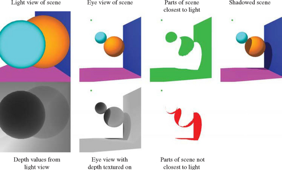
The value of the depth texture’s texel value is compared against the generated texture coordinate’s r value at each fragment. This comparison requires a special texture parameter. The comparison is used to determine whether the pixel is shadowed from the light source. If the r value of the texture coordinate is greater than the corresponding texel value, the object is in shadow. If not, it is visible by the light in question, and therefore isn’t in shadow.
This procedure works because the depth buffer records the distances from the light to every object in the scene, creating a shadow map. The smaller the value the closer the object is to the light. The texture transform and texture coordinate generation function are chosen so that x, y, and z locations of objects in the scene generate s, t, and r values that correspond to the x, y, and z values seen from the light’s viewpoint. The z coordinates from the light’s viewpoint are mapped into r values, which measure how far away a given point on the object is from the light source. Note that the r values and texel values must be scaled so that comparisons between them are meaningful. See Section 13.6 for more details on setting up the texture coordinate transformations properly.
Both the texture value and the generated r coordinate measure the distance from an object to the light. The texel value is the distance between the light and the first object encountered along that texel’s path. If the r distance is greater than the texel value, it means that there is an object closer to the light than this object. Otherwise, there is nothing closer to the light than this object, so it is illuminated by the light source. Think of it as a depth test done from the light’s point of view.
Most of the shadow map functionality can be done with an OpenGL 1.1 implementation. There is one piece missing, however: the ability to compare the texture’s r component against the corresponding texel value. Two OpenGL extensions, GL_ARB_depth_texture and GL_ARB_shadow, provide the functionality necessary. OpenGL 1.4 supports this functionality as part of the core implementation. These extensions add a new type of texture, a depth texture, that can have its contents loaded directly from a depth buffer using glCopyTexImage. When texturing with a depth buffer, the parameters GL_TEXTURE_COMPARE_MODE, GL_TEXTURE_COMPARE_FUNC, and GL_DEPTH_TEXTURE_MODE are used to enable testing between the texel values and the r coordinates. In this application, setting these parameters as shown in Table 17.4 produces shadow mapping comparisons.
Table 17.4
Texture Parameter Settings for Depth Testing
| Parameter | Value |
| GL_TEXTURE_COMPARE_MODE | GL_COMPARE_R_TO_TEXTURE |
| GL_TEXTURE_COMPARE_FUNC | GL_LEQUAL |
| GL_DEPTH_TEXTURE_MODE | GL_ALPHA |
The new functionality adds another step to texturing: instead of simply reading texel values and filtering them, a new texture comparison mode can be used. When enabled, the comparision function compares the current r value to one or more depth texels. The simplest case is when GL_NEAREST filtering is enabled. A depth texel is selected (using the normal wrapping), and is then compared to the r value generated for the current pixel location. The exact comparision depends on the value of the GL_TEXTURE_COMPARE_FUNC parameter. If the comparision test passes, a one is returned; if it fails, a zero is returned.
The texels compared against the r value follow the normal texture filtering rules. For example, if the depth texture is being minified using linear filtering, multiple texels will be compared against the r value and the result will be a value in the range [0, 1]. The filtered comparision result is converted to a normal single component texture color, luminance, intensity, or alpha, depending on the setting of the GL_DEPTH_TEXTURE_MODE parameter. These colors are then processed following normal texture environment rules.
The comparison functionality makes it possible to use the texture to create a mask to control per-pixel updates to the scene. For example, the results of the texel comparisions can be used as an alpha texture. This value, in concert with a texture environment setting that passes the texture color through (such as GL_REPLACE), and alpha testing makes it possible to mask out shadowed areas using depth comparision results. See Section 14.5 for another use of this approach.
Once alpha testing (or blending if linearly-filtered depth textures are used) is used to selectively render objects in the scene, the shadowed and nonshadowed objects can be selectively lighted, as described in Section 17.4.2 for shadow volumes.
Shadow Map Trade-offs
Shadow maps have some important advantages. Being an image-space technique, they can be used to shadow any object that can be rendered. It is not necessary to find the silhouette edge of the shadowing object, or clip the object being shadowed. This is similar to the advantages of depth buffering versus an object-based hidden surface removal technique, such as depth sort. Like depth buffering, shadow mapping’s performance bounds are predictable and well understood. They relate to the time necessary to render the scene twice: once from the light’s viewpoint and once from the viewpoint with the shadow map textured onto the objects in the scene.
Image-space drawbacks are also present. Since depth values are point sampled into a shadow map and then applied onto objects rendered from an entirely different point of view, aliasing artifacts are a problem. When the texture is mapped, the shape of the original shadow texel does not project cleanly to a pixel. Two major types of artifacts result from these problems: aliased shadow edges and self-shadowing “shadow acne” effects.
These effects cannot be fixed by simply averaging shadow map texel values, since they encode depths, not colors. They must be compared against r values, to generate a boolean result. Averaging depth values before comparison will simply create depth values that are incorrect. What can be averaged are the Boolean results of the r and texel comparison. The details of this blending functionality are left to the OpenGL implementation, but the specification supports filtering of depth textures. Setting the minification and magnification filters to GL_LINEAR will reduce aliasing artifacts and soften shadow edges.
Beyond blending of test results, there are other approaches that can reduce aliasing artifacts in shadow maps. Two of the most important approaches are shown below. Each deals with a different aspect of aliasing errors.
1. Shadow maps can be jittered. This can be done by shifting the position of the depth texture with respect to the scene being rendered. One method of applying the jitter is modifying the projection in the texture transformation matrix. With each jittered position, a new set of r/depth texel comparisons is generated. The results of these multiple comparisons can then be averaged to produce masks with smoother edges.
2. The shadow map can be biased. The bias is applied by modifying the texture projection matrix so that the r values are biased down by a small amount. Making the r values a little smaller is equivalent to moving the objects a little closer to the light. This prevents sampling errors from causing a curved surface to shadow itself. Applying a bias to r values can also be done using polygon offset to change the coordinates of the underlying geometry.
Jittering a shadow map to create a soft shadow can be done for more than aesthetic reasons. It can also mitigate an artifact often seen with shadow maps. Shadowed objects whose faces are coplanar with, and very close to the edge of a shadow map shadow can show rasterization effects similar to z-fighting. This problem is similar to the one seen with shadow volumes, but for a different reason.
In the shadow map case, geometry nearly coincident with a shadow edge will be nearly edge-on from the light’s point of view. As a result, rendering from that point of view will create an “edge” in the depth buffer, where the values change. Rasterizing the scene the second time from the eye’s viewpoint will cause that edge to be texture mapped across the face of the coincident polygons. The rasterization patterns resulting from sampling the descrete depth buffer pixels will be magnified as they are used to test against r on these polygons.
As suggested previously, this artifact can be mitigated by averaging the results of the depth tests of adjacent depth buffer samples. This can be done through a linear magnification or minification, or by jittering the light position and combining the results, producing shadows with smooth edges—in effect, “antialiasing” the shadow edges.
A more fundamental problem with shadow maps should be noted. It is difficult to use the shadow map technique to cast shadows from a light surrounded by shadowing objects. This is because the shadow map is created by rendering the a set of objects in the scene from the light’s point of view, projecting it into the depth buffer. It’s not always possible to come up with a single transform to do this, depending on the geometric relationship between the light and the objects in the scene. As a result, it can be necessary to render sections of a scene with multiple passes, each time using a different transform. The results of each pass are applied to the part of the scene covered by the transform. The solution to this problem can be automated by using a cube map depth texture to store the light point of the view in multiple directions in the faces of the cube map.
17.4.4 Creating Soft Shadows
Most shadow techniques create a very “hard” shadow edge. Surfaces in shadow and surfaces being lighted are separated by a sharp, distinct boundary, with a large change in surface brightness. This is an accurate representation for distant point light sources, but is unrealistic for many lighting environments.
Most light sources emit their light from a finite, non-zero area. Shadows created by such light sources don’t have hard edges. Instead, they have an umbra (the shadowed region that can “see” none of the light source), surrounded by a penumbra, the region where some of the light source is visible. There will be a smooth transition from fully shadowed to lit regions. Moving out toward the edge of the shadow, more and more of the light source becomes visible.
Soft Shadows with Jittered Lights
A brute-force method to approximate the appearance of soft shadows is to use one of the shadow techniques described previously and modeling an area light source as a collection of point lights. Brotman and Badler (1984) used this approach with shadow volumes to generate soft shadows.
An accumulation buffer or high-resolution color buffer can combine the shadowed illumination from multiple-point light sources. With enough point light source samples, the summed result creates softer shadows, with a more gradual transition from lit to unlit areas. These soft shadows are a more realistic representation of area light sources. To reduce aliasing artifacts, it is best to reposition the light in an irregular pattern.
This area light source technique can be extended to create shadows from multiple, separate light sources. This allows the creation of scenes containing shadows with nontrivial patterns of light and dark, resulting from the light contributions of all lights in the scene.
Since each sample contribution acts as a point light source, it is difficult to produce completely smooth transitions between lit and unlit areas. Depending on the performance requirements, it may take an unreasonable number of samples to produce the desired shadow quality.
Soft Shadows Using Textures
Heckbert and Herf describe an alternative technique for rendering soft shadows. It uses a “receiver” texture for each shadowed polygon in the scene (Heckbert, 1996). The receiver texture captures the shadows cast by shadowing objects and lights in the scene on its parent polygon.
A receiver texture is created for every polygon in the scene that might have a shadow cast on it. The texture’s image is created through a rendering process, which is repeated for every light that might cast a shadow on the polygon. First a target quadrilateral is created that fits around the polygon being shadowed, and embedded in its plane. Then a perspective transform is defined so that the eye point is at the light’s position, while the quadrilateral defines the frustum’s sides and far plane. The near plane of the transform is chosen so that all relevant shadowing objects are rendered. Once it has been calculated, objects that might shadow the polygon are rendered using this transform.
After the transform is loaded, the rendering process itself is composed of two steps. First, the shadowed polygon itself is rendered, lighted from one of the light sources that could cast a shadow on it. Then every other object that may shadow the polygon is rendered, drawn with the ambient color of the receiving polygon. Since all shadowing objects are the same color, the painter’s algorithm will give correct results, so no depth buffering is needed. This is a useful feature of this algorithm, since turning off depth buffering will improve performance for some OpenGL hardware implementations. The resulting image is rendered at the desired resolution and captured in a color buffer with high pixel resolution, or the accumulation buffer if performance is less of a factor.
The process is repeated for every point light source that can illuminate the shadowed polygon. Area lights are simulated by sampling them as numerous point light sources distributed over the area light’s face. As every image is rendered, it is accumulated with the others, adding them into the total light contribution for that polygon. After all images have been accumulated, the resulting image is copied to a texture map. When completed, this texture is applied to its polygon as one of its surface textures. It modulates the polygon’s brightness, modeling the shadowing effects from its environment.
Care must be taken to choose an appropriate image resolution for the receiver texture. A rule of thumb is to use a texture resolution that leads to a one-to-one mapping from texel to pixel when it is applied as a surface texture. If many accumulation passes are necessary to create the final texture, the intensity of each pass is scaled so as to not exceed the dynamic range of the receiving buffer. There are limits to this approach as color values that are too small may not be resolvable by the receiving buffer.
A paper describing this technique in detail and other information on shadow generation algorithms is available at Heckbert and Herf’s web site (Heckbert, 1997). The Heckbert and Herf method of soft shadow generation is essentially the composition of numerous “hard” shadow visibility masks. The contributions from individual light positions will be noticeable unless sufficient number of light source samples are used. The efficiency of this method can be increased by adjusting the number of samples across the shadow, increasing the number of samples where the penumbra is large (and will produce slowly varying shadow intensities).
Soler and Sillion (Soler, 1998) proposed another method to reduce soft shadow artifacts. Their method models the special case where the light source, shadow occluder, and shadow receiver are all in parallel planes. They use a convolution operation that results in shadow textures with fewer sampling-related artifacts. In essence, they smooth the hard shadows directly though image processing, rather than relying soley on multiple samples to average into a soft shadow.
First, the light source and shadow occluder are represented as images. Scaled versions of the images are then efficiently convolved through the application of the Fast Fourier transform (FFT) and its inverse to produce a soft shadow texture. Soler and Sillion go on to apply approximations that generalize the “exact” special case of parallel objects to more general situations. While the FFT at the heart of the technique is not readily accelerated by OpenGL, convolution can be accelerated on implementations that support the ARB imaging extension or fragment program, which can produce similar results. Even without convolution, the technique can still be useful in interactive applications. It’s approach can be used to precompute high-quality shadow textures that can later be used like light map textures during OpenGL rendering.
17.5 Summary
This chapter covered some important and fundamental approaches to realism, with an emphasis on inter-object lighting. Reflections, refractions, environment map creation, and shadowing were covered here. Modeling these effects accurately is key to creating realistic scenes. They often give the strongest impact to visual realism, after considering the surface texture and geometry of the objects themselves. To obtain still higher levels of realism, the application designer should consider augmenting these approaches with fragment programs.
Fragment programs are rapidly becoming the method of choice for augmenting scene realism. Although computationally expensive, the ability to create surface “shaders” is a powerful method for creating detailed surfaces, and with good environment maps can model interobject reflections realistically. Although not part of any core specification at the time of this writing, it is rapidly evolving into an indispensible part of OpenGL. For more information on fragm ent programs, consult the specification of the ARB_fragm ent_program extension, and descriptions of higher-level APIs, such as GLSL.
1Part of core OpenGL 1.4.