
CHAPTER
13
Tools of the Trade
In malware analysis, it is important to have the right tools. Familiarity with these tools and how to use them properly is the difference between success and failure in malware analysis. The use of tools to perform malware analysis has been discussed throughout this book. In previous chapters, I discussed how to use certain tools to perform static and dynamic malware analysis.
The right tools together with the right skills are a powerful combination when faced with a difficult malware to analyze.
In this chapter, you will take a look at more tools that are important when it comes to malware analysis. I consider them tools of the trade.
Malware Analysis Use Cases
When it comes to tool selection, it is important to understand first what you want to do and then choose the appropriate tool for the job. For example, if you want to know the file type of a suspicious file, you know that you can use PEiD or the Linux file command line. But if one of the things you want to do is to have the ability to add signatures so the tool can detect new file types or characterize a file based on your need, the best tool for the job is PEiD.
The choice of the tool, therefore, must be dictated by what you want to accomplish. What you want to accomplish is also known as a malware analysis use case. You must choose your tool or a set of tools based on satisfying your malware analysis use cases.
The following are some examples of malware analysis use cases:
![]() Ability to determine whether a file is packed
Ability to determine whether a file is packed
![]() Ability to unpack a packed binary
Ability to unpack a packed binary
![]() Ability to determine file system changes done by malware
Ability to determine file system changes done by malware
![]() Ability to determine registry changes done by malware
Ability to determine registry changes done by malware
![]() Ability to dump memory contents of an infected system
Ability to dump memory contents of an infected system
![]() Ability to determine a malware’s network connections
Ability to determine a malware’s network connections
![]() Ability to determine what data is being exfiltrated by malware
Ability to determine what data is being exfiltrated by malware
In one way or another, you were able to satisfy these use cases in previous chapters.
Malware Analyst Toolbox
As a malware analyst, having a toolbox is important. What makes up this toolbox is dependent upon your malware analysis use cases. If you are a security professional, your use cases are dictated by your research tasks or operational tasks. If you are a hobbyist, your use cases are dictated by what you want to learn or do when it comes to malware analysis. Regardless of your use cases, there are some tools that are indispensable. I call these tools the tools of the trade.
Tools of the Trade
The following are some of the tools I consider to be important when it comes to malware analysis:
![]() Sysinternals Suite
Sysinternals Suite
![]() Yara
Yara
![]() Cygwin
Cygwin
![]() Debuggers
Debuggers
![]() Disassemblers
Disassemblers
![]() Memory dumpers
Memory dumpers
![]() PE viewers
PE viewers
![]() PE reconstructors
PE reconstructors
![]() Malcode Analyst Pack
Malcode Analyst Pack
![]() Rootkit tools
Rootkit tools
![]() Network capturing tools
Network capturing tools
![]() Automated sandboxes
Automated sandboxes
![]() Free online automated sandbox services
Free online automated sandbox services
Sysinternals Suite
As discussed in previous chapters, Sysinternals is an indispensible tool. It comes as a suite containing all the tools, or you can download each tool separately if you do not want to get the whole package.
You can download the suite from https://technet.microsoft.com/en-us/sysinternals/bb842062.aspx, and if you want to download just a specific tool from the suite, simply click the name of the tool you want from the page pointed to by the link, and you will be all set.
Yara
Yara is a versatile pattern-matching tool. As claimed on its website, it is indeed the pattern-matching Swiss Army knife for malware researchers and everyone else. Yara is a tool aimed at, but not limited to, helping malware researchers to identify and classify malware samples. With Yara, you can create descriptions of malware families or whatever you want to describe based on textual or binary patterns.1
A description is also known as a Yara rule. Each rule consists of a set of strings and a Boolean expression, which determines its logic. The strings, which comprise the textual or binary patterns, are then used as signatures to detect a possible match based on the logic written in the rule.
Figure 13-1 is an example of a Yara rule taken from https://github.com/plusvic/yara.

Figure 13-1 Example Yara rule.
The first line contains the keyword rule, which means that what follows is a Yara rule. The string after it, which is silent_banker, is the name of the rule. If a binary or file that is scanned matches this specific rule, that file will be labeled as silent_banker. The string after the colon is a grouping. This means that the rule named silent_banker is part of the group banker. The grouping name is not displayed when a match is found.
The meta section includes a description of the rule. This is merely an aid for Yara rule creators. Think of it as a comment section.
The strings section contains the strings that serve as the signature. It can be in hexadecimal or text.
The condition section contains the logic of the rule. It contains a Boolean expression telling how the rule will be satisfied. In the example in Figure 13-1, if any of the strings are found in the file, the rule is satisfied, and the file is considered a match for silent_banker.
Think of a Yara rule as the signature and Yara as the engine. It works similar to a traditional file scanner or antivirus program.
To get started with Yara, read the full documentation at http://yara.readthedocs.org/en/v3.3.0/, or you can simply go to https://plusvic.github.io/yara/ and click Read The Documentation on the right side of the page. From this link you can also download the latest release, send bug reports, and ask for help from Yara’s group.
In this lab, you will install Yara on a system running in Ubuntu.
What You Need:
![]() System running Ubuntu 14.04.1
System running Ubuntu 14.04.1
![]() Yara
Yara
Steps:
1. Download Yara from https://github.com/plusvic/yara/releases/tag/v3.3.0 or go to https://plusvic.github.io/yara/ and click Download Latest Release on the right side of the page. As of this writing, the latest version is Yara 3.3.0. Since you are using Ubuntu, download the source code (tar.gz) under the Downloads section. This is the source tarball.
2. The file that will be downloaded is yara-3.3.0.tar.gz.
3. Open a terminal window and go to the folder where yara-3.3.0.tar.gz was downloaded.

5. If the command ./bootstrap.sh spews out any kind of error regarding autoreconf, issue the following command line to install autoconf and libtool:
![]()
6. Run bootstrap.sh again.
![]()
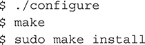
7. After a successful run of bootstrap.sh, issue the following commands:
8. Another way of installing Yara is by issuing the following command line:
![]()
9. Type the following command line to check whether Yara was installed successfully:
![]()
10. If the help section of Yara is displayed, you now have Yara successfully installed on your system.
In this lab, you will create your first Yara rule.
What You Need:
![]() System running Ubuntu 14.04.1
System running Ubuntu 14.04.1
![]() Yara
Yara
![]() Calc.EXE from Windows
Calc.EXE from Windows
Steps:
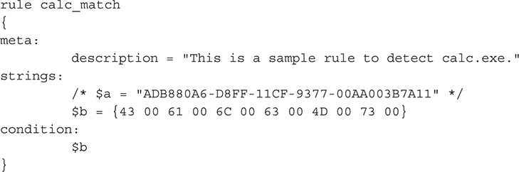
1. Create a new text file and type the following:

2. The previous strings make up the file’s CLSID found in file offset 0x9A7. It might be different from the CLSID that your Calc.EXE has. To check, run the following command line, browse to the mentioned offset, and adjust the rule appropriately. It is also possible that the CLSID is found in a different offset.
![]()
3. Save the text file as yara_rule.txt.
4. Issue the following command:
![]()
The first argument is the rule file, and the second argument is the file to be scanned.
5. If the strings match what is in the file, the following output is displayed:
![]()
calc_match is the name of the rule, and calc.exe is the file that matches it.
6. Open the yara_rule.txt file and add another string from file offset 0x6F0. But instead of using its text equivalent, use hex values representing the string. Change the condition to $b, which means that the rule will use only $b as the matching string. Comment out the $a string using /* and */ and then save the file.
7. Run Yara to check for a match. If the strings are written correctly, there will be a positive match.
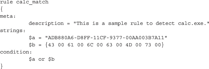
8. Open the yara_rule.txt file, uncomment the $a string, and modify the condition to $a or $b. This means that if any of the strings are present in the file, it will be a positive match. The final rule will look like this:
9. For more about Yara writing rules, visit http://yara.readthedocs.org/en/v3.3.0/writingrules.html.
In this lab, you will install Yara support for Python so you can utilize it in a Python script.
What You Need:
![]() System running Ubuntu 14.04.1
System running Ubuntu 14.04.1
![]() Yara
Yara
![]() Python
Python
Steps:
1. Install python-dev using the command line in a terminal window.
![]()
2. Build and install the yara-python extension. From the terminal window, go to the folder where Yara was extracted. From Lab 13-1, the folder is yara-3.3.0. The folder name changes based on the version of Yara you downloaded. As of this writing, the latest is 3.3.0. From inside the yara-3.3.0 folder, issue the following commands:

3. To avoid an ImportError in Ubuntu, add the path /usr/local/lib to the loader configuration file by issuing the following command line:
![]()
4. If the command line is not letting you make the necessary changes to /etc/ld.so.conf, you can use gedit as an alternative. From a terminal window, issue the following commands:
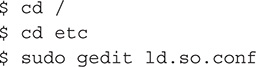
5. Add the line /usr/local/lib without the quotes at the end of the file.
6. Save and close the file.
7. In the terminal window, run the command to load the config file.
![]()
8. To check for successful installation, run the Python development environment by issuing the following command line:
![]()
9. In the development environment, issue the following command:
![]()
10. If there are no errors, this means that the installation is successful. Type exit() to exit the development environment.
![]()
In this lab, you will create a Python script that utilizes Yara rules to classify files.
What You Need:
![]() System running Ubuntu 14.04.1
System running Ubuntu 14.04.1
![]() Yara
Yara
![]() Python
Python
![]() Calc.EXE from Windows
Calc.EXE from Windows
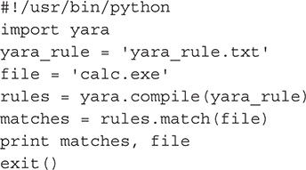
1. Create a Python script file and write the following code:
2. After creating the Python script, change it to executable mode by issuing the following command:
![]()
3. Execute your script. Make sure that yara_rule.txt and calc.EXE are in the same folder as your script.
![]()
4. The output will look like the following:
![]()
5. You can find more about using Yara with Python at http://yara.readthedocs.org/en/v3.3.0/yarapython.html.
Cygwin
Cygwin is a tool that gives you that Linux feeling in Windows. Cygwin is a large collection of GNU and open source tools that provide functionality similar to a Linux distribution in Windows. But it is not a way to run native Linux apps on Windows nor is it a way to magically make Windows programs aware of Unix functionalities. Instead, Cygwin is a DLL that provides substantial POSIX application programming interface (API) functionality.2 The Cygwin DLL is cygwin1.dll.
Cygwin provides a quick and easy way for analysts to have access to some GNU command lines from Windows without switching operating systems.
In this lab, you will install Cygwin in a Windows box, specifically Window 7.
What You Need:
![]() System running Windows 7
System running Windows 7
![]() Cygwin
Cygwin
Steps:
1. Download Cygwin from https://www.cygwin.com. For this purpose, you will be downloading the 64-bit version. The downloaded file is setup-x86_64.exe.
2. Install Cygwin and follow the prompts. Figure 13-2 shows the installation window of Cygwin. Click Next.

Figure 13-2 Cygwin installation window.
3. In the next window, choose Install From Internet. This is the default. Click Next.
4. Choose the root directory of Cygwin. For this purpose, you will stick with the default, which is C:cygwin64. You will also install for All Users, which is the default. Click Next.
5. Choose where to put the local package. This stores all the installation files for future use. Click Next.
6. Select the appropriate Internet connection for download. A direct connection is the default connection. Click Next.
7. Choose a download site. If you have your own user uniform resource locator (URL) such as from your university or work that hosts Cygwin, it is advisable to use that one. Click Next.
8. The installer will parse the mirror for packages. If the speed is slow, you can always cancel the installation, restart it, and choose a different download site.
9. Once parsing is complete and available packages have been identified, you will be asked to choose the packages you want to install. Installing all packages is the default. Simply remove the packages you don’t want. But for the purpose of this lab, you will install all packages. Click Next.
10. If there are dependencies needed by any of the packages, Cygwin will resolve them by installing the required packages to satisfy dependencies. Click Next.
11. The installer will begin downloading and installing the packages. This may take some time. Once this is done, click Next.
12. Choose whether you want to have icons on your desktop, Start menu, or both. Click Finish.
13. Installation is now complete. You now have Cygwin Terminal, as shown in Figure 13-3.

Figure 13-3 Cygwin Terminal window.
14. Treat Cygwin as you would have a terminal window in Linux-based systems.
15. For more information, read Cygwin’s documentation at https://cygwin.com/docs.html.
TIP
To update Cygwin, simply run the installer again.
Debuggers
In computer science, debugging is the process of finding errors or bugs in a program or a device. The tools that are used for debugging are called debuggers. In DOS, a reliable tool for this is Debug.COM, but the world of debuggers has come a long way after that.
In malware analysis, debugging is the process of tracing code to find out what it does. It is a step-by-step tracing of malware code to determine its true intention. This is why debugging is a critical ingredient of reverse engineering.
For the purpose of this book, debugging is a helpful process to determine whether a binary is encrypted, packed, or neither. Learning this skill is needed, especially if the packer or cryptor is new and no PEiD or Yara signature exists yet to detect it. Remember, any file that is encrypted or packed usually renders static analysis useless. But if a malware is unpacked or decrypted through the use of tools, it will be easy to get information from it using static analysis; thus, you have more data to help you classify whether a file is malicious and even cluster it with its group or malware family for better identification.
The following are most common debuggers that are used in malware analysis:
![]() OllyDbg
OllyDbg
![]() Immunity Debugger
Immunity Debugger
![]() Windows Debuggers
Windows Debuggers
OllyDbg
OllyDbg is a classic tool that is still popular with malware analysts today. You can download it from http://www.ollydbg.de/. One great thing about OllyDbg, called Olly for short, is that there is a wealth of plug-ins available for download all over the Internet to make debugging easier. A search for OllyDbg plug-ins will yield lots of resources when it comes to useful plug-ins. But as with other things available freely on the Web, exercise caution when downloading and using them.
Immunity Debugger
Immunity Debugger is a debugger that boasts of features that are deemed friendly for security experts. You can download it from http://debugger.immunityinc.com/. On its main page, it is described as a powerful new way to write exploits, analyze malware, and reverse engineer binary files. It can also be extended by using a large and well-supported Python API.
Windows Debuggers
The most common Windows debuggers are WinDbg, KD, and NTKD. The one that encompasses all, at least in my humble opinion, is WinDbg. WinDbg is Microsoft’s own Windows debugger. It is part of the Windows Driver Kit, but it can also be downloaded as a stand-alone tool from https://msdn.microsoft.com/en-us/windows/hardware/hh852365.aspx.
WinDbg is thought to have an “inside” advantage compared to other debuggers because it is written specifically for Windows. It has the following features:
![]() Kernel mode debugging
Kernel mode debugging
![]() User mode debugging
User mode debugging
![]() Managed debugging
Managed debugging
![]() Unmanaged debugging
Unmanaged debugging
![]() Ability to attach to a process
Ability to attach to a process
![]() Ability to detach from a process
Ability to detach from a process
It basically covers all the bases of other Windows debuggers such as KD and NTKD. You can find more information about KD and NTKD from https://msdn.microsoft.com/en-us/library/windows/hardware/hh406279%28v=vs.85%29.aspx.
Disassemblers
A disassembler is a tool that breaks down a binary into assembly code. A disassembler is often used in tandem with a debugger. A debugger follows the assembly code in memory, and the output of the disassembler serves as a map or a good indicator whether the code being traced in memory is still in line with the disassembled code. Sometimes there will be differences, which means that either the debugging session is going to a dead end or the disassembled code is not as reliable probably because the malware has an anti-disassemble capability.
The most popular disassembler is IDA. It is also considered a debugger. IDA is a little pricey, but the good thing about it is that there is always a free version available that is for non-commercial use. You can download it from https://www.hex-rays.com/products/ida/support/download.shtml.
IDA is a powerful tool. I suggest downloading a free copy of it and playing around with it. There are lots of resources from its website that will help you get started. The more you use it, the better you will become at using IDA.
Memory Dumpers
Memory dumpers are tools that dump a running process from memory. There are a handful of process dumpers available such as Microsoft’s ProcDump, but the most useful tools, in my humble opinion, when it comes to malware analysis are LordPE and Volatility.
LordPE
LordPE is a tool that can dump a process from memory and has the ability to edit basic PE header information. You can download the tool from http://www.woodmann.com/collaborative/tools/index.php/LordPE.
Volatility Framework
Volatility is a free, useful memory dump analyzer. It is a single, cohesive framework that supports 32-bit and 64-bit Windows, Linux, Mac, and Android systems. It is a Python-based framework that allows users to analyze an OS environment from a static dump file. Being Python-based makes Volatility versatile. It can be programmed to do almost anything a memory dump analyzer can do. To get started on Volatility, visit https://code.google.com/p/volatility/wiki/VolatilityIntroduction.
PE Viewers
PE viewers are tools that provide a glimpse of a PE file. There are lots of PE viewers available depending on your needs. The following are some of them:
![]() Hiew
Hiew
![]() Heaventools PE Explorer
Heaventools PE Explorer
![]() PEview
PEview
![]() Dependency Walker
Dependency Walker
![]() Resource Hacker
Resource Hacker
Hiew
Hiew is a classic PE viewer. It has the ability to not only view and edit files of any length in text and hex but also disassemble a PE file. Some of the features are as follows:
![]() x86-64 disassembler and assembler
x86-64 disassembler and assembler
![]() View and edit physical and logical drive
View and edit physical and logical drive
![]() Pattern search in disassembler
Pattern search in disassembler
![]() Built-in simple 64-bit decrypt/crypt system
Built-in simple 64-bit decrypt/crypt system
![]() Block operations: read, write, fill, copy, move, insert, delete, crypt
Block operations: read, write, fill, copy, move, insert, delete, crypt
![]() Multifile search and replace
Multifile search and replace
![]() Unicode support
Unicode support
You can find more information about the tool at http://www.hiew.ru/.
Heaventools PE Explorer
PE Explorer has all the capabilities of a typical PE viewer. The following are the extra features it offers:
![]() API function syntax lookup
API function syntax lookup
![]() Dependency scanner
Dependency scanner
![]() Section editor
Section editor
![]() Unpacker support for UPX, Upack, and NsPack
Unpacker support for UPX, Upack, and NsPack
PE Explorer is not free, but it offers a 30-day trial version. You can download it from http://www.heaventools.com/overview.htm.
PEview
PEview, as stated on its website, provides a quick and easy way to view the structure and content of PE and COFF files. It displays header, section, directory, import table, export table, and resource information within EXE, DLL, OBJ, LIB, DBG, and other file types. You can download it from http://wjradburn.com/software/.
Dependency Walker
Dependency Walker, as discussed in previous chapters, is a free utility that scans any 32-bit or 64-bit Windows module and builds a hierarchical tree diagram of all dependent modules.
You can download Dependency Walker from http://www.dependencywalker.com/.
Resource Hacker
Resource Hacker is a freeware utility to view, modify, rename, add, delete, and extract resources in 32-bit and 64-bit Windows executables and resource files. It incorporates an internal resource script compiler and decompiler and works on all Windows operating systems, at least up to Windows 7.
You can download Resource Hacker from http://www.angusj.com/resourcehacker/.
PE Reconstructors
PE reconstructors are tools that have the ability to reconstruct a portable executable file from memory or from a dump file given that these tools have all the information they need such as the entry point, relative virtual address, and size. The most common PE reconstructor used in malware analysis is ImpREC by MackT. It has the ability to rebuild the import address table (IAT) from a memory dump. You can download the tool from http://www.woodmann.com/collaborative/tools/index.php/ImpREC.
The tools discussed so far are stand-alone, and each has their own purpose. Combining their use to solve a malware analysis problem or use case is not a foreign idea. For example, manually unpacking a malware is one problem that all malware analysts and researchers have faced throughout the years. The right combination of tools can help a malware analyst and researcher break a packed or encrypted malware.
In this lab, you will use the different tools discussed so far to manually unpack a packed malware. The malware that you will use specifically for this lab has the following characteristics:
![]() MD5 c0c9c7ea235e4992a67caa1520421941
MD5 c0c9c7ea235e4992a67caa1520421941
![]() SHA1 da39a3ee5e6b4b0d3255bfef95601890afd80709
SHA1 da39a3ee5e6b4b0d3255bfef95601890afd80709
![]() SHA256 e3b0c44298fc1c149afbf4c8996fb92427ae41e4649b-934ca495991b7852b855
SHA256 e3b0c44298fc1c149afbf4c8996fb92427ae41e4649b-934ca495991b7852b855
What You Need:
![]() Debuggers
Debuggers
![]() Disassemblers
Disassemblers
![]() Static analysis tools
Static analysis tools
![]() Dynamic analysis tools
Dynamic analysis tools
![]() System running Windows
System running Windows
![]() Packed malware
Packed malware
Steps:
1. The first thing to do is to use PEiD to determine whether it is packed.
2. Figure 13-4 shows the output of PEiD. As you can see, PEiD did not detect anything. Even its Entropy shows that the file is not packed.

Figure 13-4 PEiD output.
3. Let’s try PEView. Figure 13-5 shows the output. You can see in the IAT that there are many imports, which oftentimes depict that the file is unpacked and everything looks normal.
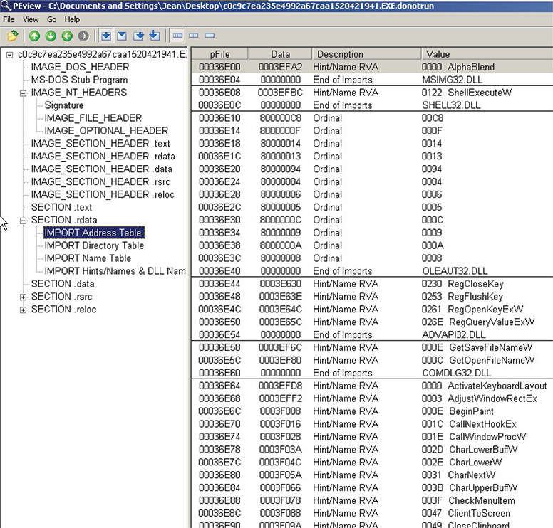
Figure 13-5 PEView output.
4. Let’s try IDA. Figure 13-6 shows the output. From here, you can see that there is only one function, the start function. Close to the end of the start function there is a CALL instruction to a value stored in the stack. The value is the return value of the function InverRect that was called before, and its return value plus 27C8Ah was stored on the stack. With this information, you come into the conclusion that this file is packed after all, even if PEiD and PEView say otherwise.

Figure 13-6 IDA output.
5. At this point, you need to drop the file into a debugger, look at the assembly instructions, and attempt to unpack the file.
6. In this lab, you will be using Immunity Debugger. Figure 13-7 shows the debugging session of the packed file in Immunity Debugger.

Figure 13-7 Immunity Debugger session.
The general approach with unpacking is to step over calls and not step into function calls unless you have a good reason to do it. Also, make a lot of snapshots every time you are stepping over a call you are not sure about. This will allow you to revert to your last position in an instant when needed.
7. In Immunity Debugger, you start off at the entry point. Scrolling down a bit reveals some calls to legitimate functions such as GetConsoleOutputCP, GetDriveTypeW, InvertRec, and GlobalAddAtomW.
8. Step over the instructions by pressing F8 until you get a CALL instruction at <ModuleEntryPoint> + 196, which calls to an address that is stored in the local variable EBP-68 in the stack. Figure 13-8 shows this session.
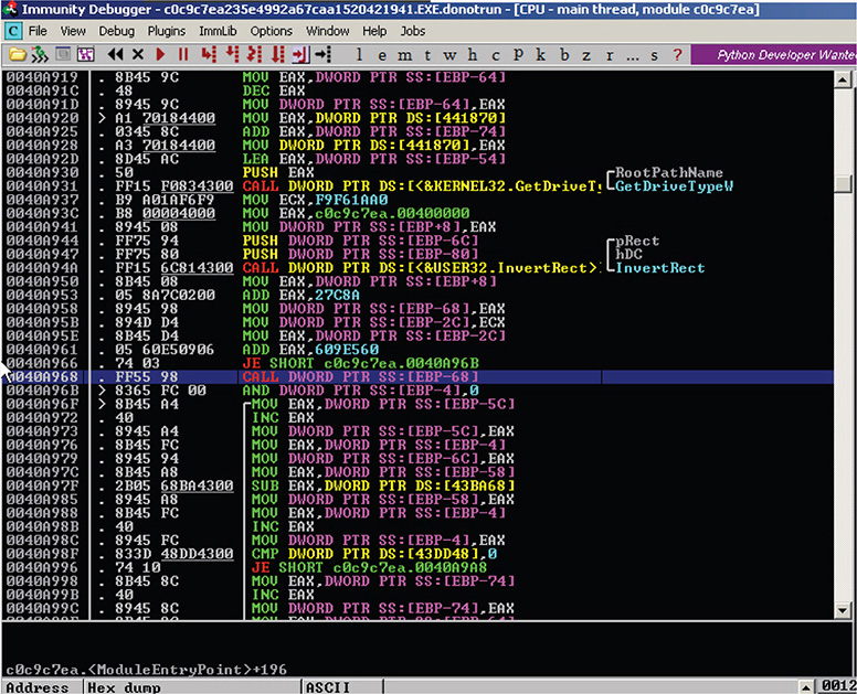
Figure 13-8 Immunity Debugger session reaching desired CALL instruction.
9. In this specific case, the address points to 0x00427C8A, but this is not necessarily the same address every time the binary is loaded. This is where you left your sample in IDA. Step into this CALL by pressing F7. Figure 13-9 shows the resulting session.

Figure 13-9 Immunity Debugger session in address 0x427C8A.
10. After stepping in, what you see (Figure 13-9) looks like obfuscated or scrambled code, which is common with packed files.
11. Following the jump brings you to the session shown in Figure 13-10.
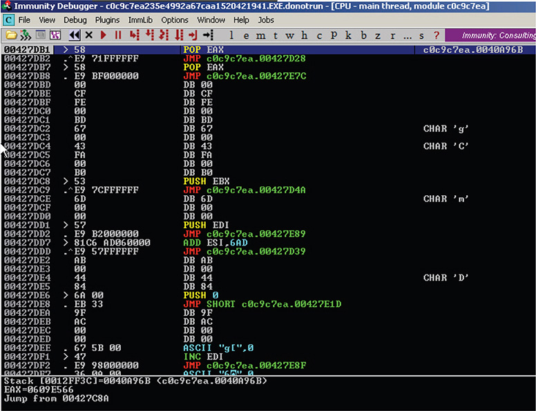
Figure 13-10 Immunity Debugger session following the JMP instruction.
12. After stepping over JMP and PUSH instructions, you will reach a CALL EAX instruction, as shown in Figure 13-11. The instructions are generally suspicious, and in some cases you will want to step in, but in this case, this is actually a dynamic call to VirtualProtect, which is used to conceal its true purpose. The permissions of the sections in the addresses 0x00400000–0x00442000 (PE Headers + .text section) is changed to RWE (Read Write Execute) so that the binary will be able to change its own code by writing a new “unpacked” version of itself to the .text section.
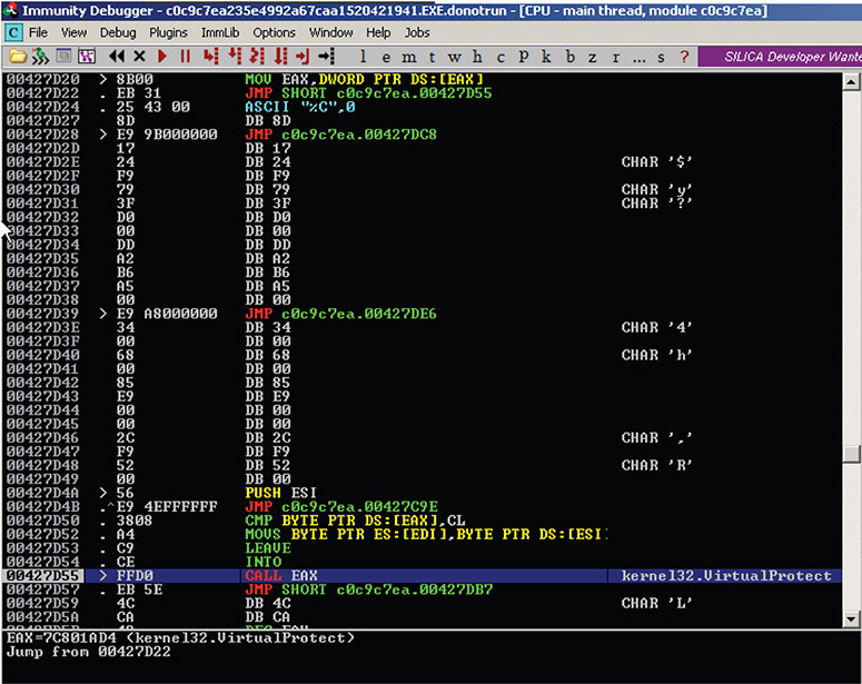
Figure 13-11 Immunity Debugger session reaching CALL EAX instruction.
13. The memory map shown in Figure 13-12 displays the current permissions of each section in memory.

Figure 13-12 Memory map.
14. Continue stepping over more JMP instructions. You can also use the animate over (CTRL+F8) feature for this purpose but not before making a snapshot.
15. After trying to animate over, you will notice the JMPs make it too difficult to follow, and thus a new approach is needed. You may have noticed that you stumbled upon the same CMP ECX, ESI instruction quite a few times while stepping over, so it seems that this is obfuscated code that might repeat itself in a loop 2,950 times. The number 2,950 comes from the hex value B86, which is the value of ESI, as shown in Figure 13-13.
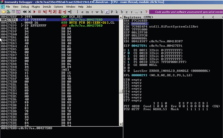
Figure 13-13 Immunity Debugger session showing ESI value.
16. To skip doing the stepping over 2,950 times, you will be setting a conditional breakpoint (CTRL+T) and use a trace over (CTRL+F12), as shown in Figure 13-14. You set the value of ECX to B86.

Figure 13-14 Conditional breakpoint and trace over.
17. Once ECX reaches the value of B86, the resulting session is as shown in Figure 13-15.
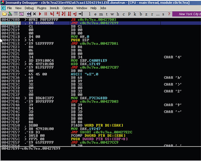
Figure 13-15 Immunity Debugger session after the breakpoint.
18. Take the JMP instruction to reach a new section in the code, as shown in Figure 13-16.
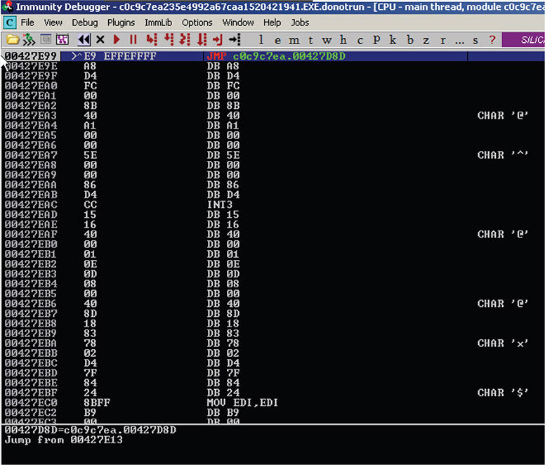
Figure 13-16 Immunity Debugger session after taking the JMP instruction.
19. Keep stepping over the instructions until you reach a JMP EAX instruction, as shown in Figure 13-17.
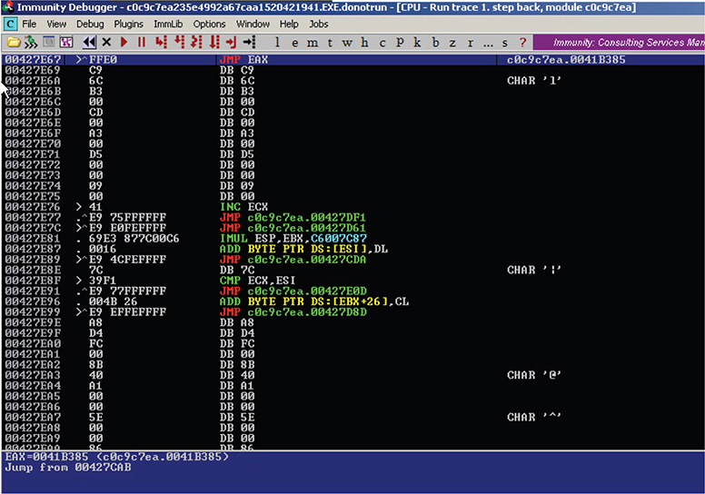
Figure 13-17 Immunity Debugger session reaching JMP EAX.
20. There is an alternative strategy to reaching this JMP EAX instruction. Assuming that the packer is trying to hide any JMP to the deobfuscated code, a good bet is that it will call a function using a CALL EAX/JMP EAX instruction. With that logic in mind, you can search (CTRL+F) for a CALL EAX/JMP EAX instruction and set a breakpoint (F2) on that instruction. Before pressing F9 to run, make sure you create a snapshot.
21. The JMP EAX takes you to 0x0041B385, as shown in Figure 13-18.

Figure 13-18 Immunity Debugger session reaching address 0x0041B385.
22. At this point, you click the current instruction and then choose Analysis | Analyse Code (CTRL+A), as shown in Figure 13-19.
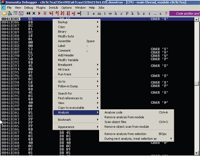
Figure 13-19 Immunity Debugger Analyse Code menu option.
23. The result, as shown in Figure 13-20, looks like a function prologue setting up the stack frame. The code looks readable. Could this be the original entrypoint (OEP) of the original packed binary?
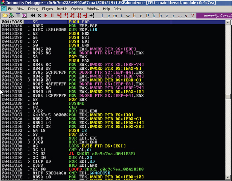
Figure 13-20 Immunity Debugger result from Analyse Code function.
24. Keep stepping over to find out. Whenever you hit a loop, set a breakpoint (F2) right after it, press F9 (Run) until the breakpoint (BP), take the BP off, and keep stepping over instructions. Figure 13-21 shows this session.

Figure 13-21 Immunity Debugger session hitting a loop.
25. When you scroll down, you will see function names as strings in the code, as shown in Figure 13-22.
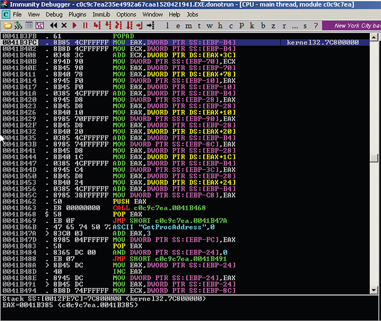
Figure 13-22 Function names as strings in the code.
26. At this point, you come to the conclusion that this is still the packer code. Or is it the unpacker code? It looks like the packer is a string pointer to function names in the KERNEL32.DLL library by using GetProcAddress. This is done by the packer so it won’t have to call these functions explicitly and there will be no trace of these functions in the IAT.
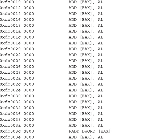
Specifically, the following instructions get string pointers to the function names embedded in the code:

In this snippet, the CALL instruction pushes the next instruction’s address, which is found in the EIP to the stack, and jumps to the function’s address, which in this case is the address of the next instruction, POP EAX. After executing the next instruction POP EAX, EAX will contain the address of the POP EAX instruction, which is just 3 bytes before the string that contains a function name. The next instruction is an unconditional jump instruction (JMP) that jumps over the string. The next instruction that will be executed is ADD EAX, 3. After the execution of this instruction, EAX will be pointing to a null-terminated string containing the function name.
This technique is repeated in a loop for many functions that are actually used by the malware but were hidden by the packer such as GetModuleHandleA, GetOutputDebugString, and so on. The function names are saved in local variables so they can be accessed later when the IAT is reconstructed in memory.
Figure 13-23 shows this whole thing in the session.
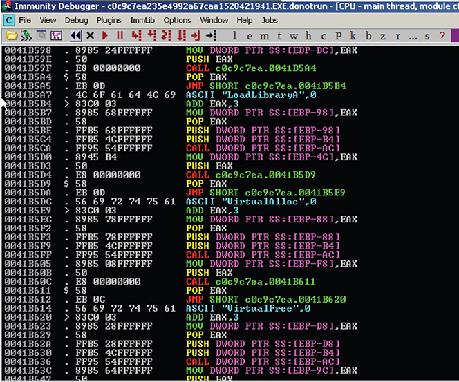
Figure 13-23 Immunity Debugger session showing string pointer technique.
27. Continue stepping over the instructions until you hit JMP EAX, as shown in Figure 13-24.

Figure 13-24 Immunity Debugger session showing JMP EAX being reached.
28. After the JMP, you come across the same technique once again, but this time the string containing the function name is hidden better. Also, notice that the JMP instruction is jumping to an unaligned address. This means that the code will get a different meaning after the jump. Figure 13-25 shows this session.

Figure 13-25 Immunity Debugger session showing the same technique but in an unaligned address.
29. Keep going until instruction ADD EAX, 3 is revealed, as shown in Figure 13-26.
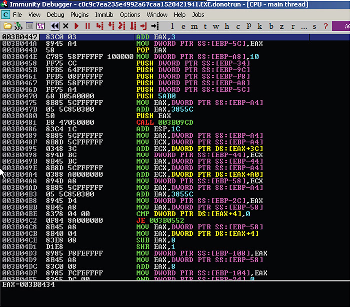
Figure 13-26 Immunity Debugger session after the ADD EAX, 3 instruction is revealed.
30. Keep stepping over until you reach the infamous technique’s set of instructions again.
The session in Figure 13-27 shows the sets of instructions.

Figure 13-27 Immunity Debugger session showing the infamous technique.
31. After the jump, you should see the instruction ADD EAX, 3; also, the “magic jump” JMP EAX should be revealed. Figure 13-28 shows this session.
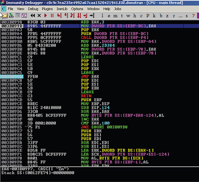
Figure 13-28 Immunity Debugger session showing ADD EAX, 3 and JMP EAX.
32. But just before you reach the magic jump, you might have one last obstacle, a CALL to OutputDebugStringA, as shown in Figure 13-29. OutputDebugStringA is sometimes used as an anti-debugging technique.
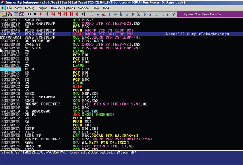
Figure 13-29 Immunity Debugger session showing CALL to OutputDebugStringA.
33. The actual function is typically used to output a string value to the debugging data stream, which will then display the debugger. OutputDebugString() acts differently based on the existence of a debugger on the running process. If a debugger is attached to the process, the function will execute normally, and no error state will be registered. However, if there is no debugger attached,
LastError will be set by the process, letting you know that you are debugger free. Malware authors can use this to change the execution flow of the malware if a debugger is detected. For the malware author to do this, she would typically use the following implementation:
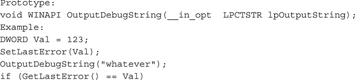

Luckily for you, it was not implemented correctly as an anti-debugging mechanism, and there is no distinction between the two cases, debugger attached or not.
34. You take the jump and get to a new section, as shown in Figure 13-30.
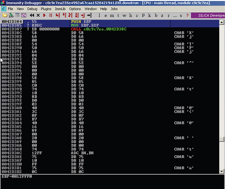
Figure 13-30 Immunity Debugger session after taking the jump.
35. Analyze the code, as shown in Figure 13-31.
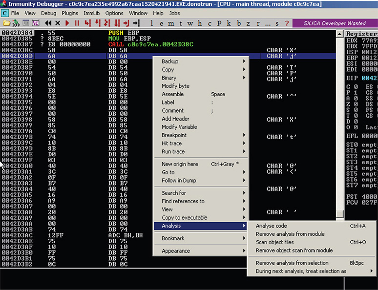
Figure 13-31 Analyze the code in Immunity Debugger.
36. The OEP is found, as shown in Figure 13-32.

Figure 13-32 OEP found in Immunity Debugger.
37. At this point, you need to dump the memory so you can get the unpacked image of the binary. For this purpose, you will use LordPE. For LordPE to be able to attach to a process, it must be run in administrator mode, and then you pick the process that you would like to dump.
38. Once you find the process that you would like to dump, right-click it, choose Dump Full, and choose a location where to save it. See Figure 13-33 showing this process.
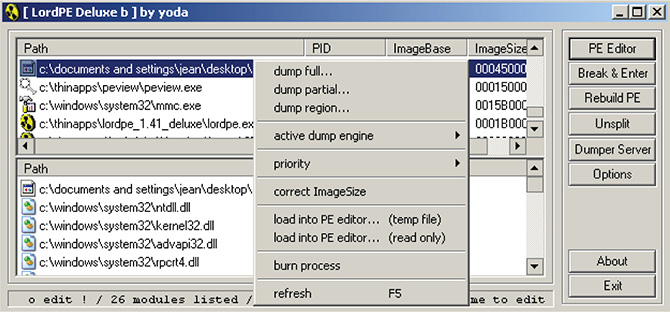
Figure 13-33 LordPE dumping a desired process.
39. After dumping the process, you can use LordPE’s PE Editor to overwrite the entry point and other PE headers depending on the sample. The button to invoke PE Editor is in the upper-right corner of LordPE. PE Editor will need you to choose a valid PE file to work on. Choose the file you saved while dumping the process from memory. Figure 13-34 shows the result when the file is loaded using LordPE’s PE Editor.

Figure 13-34 Dumped process loaded into LordPE’s PE Editor.
40. Once the file is loaded successfully, overwrite the EntryPoint value, as shown in Figure 13-35, with the RVA of the OEP you found. The RVA of the OEP is 42D384 – 400000 = 2D384.

Figure 13-35 EntryPoint value modified to reflect RVA of OEP.
41. Check the sections were not corrupted by checking that their Virtual Offset (VOffset) and Virtual Size (VSize) values match their Relative Offset (ROffset) and Relative Size (RSize) values. As you can see in Figure 13-36, all the values match for each one of the sections.

Figure 13-36 Section table of the dumped process.
42. At this point, you will use ImpREC to rebuild the IAT. Execute ImpREC and attach the malware process, as shown in Figure 13-37.
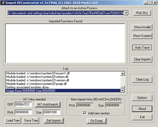
Figure 13-37 Malware process attached to ImpREC.
43. Change the OEP to the RVA of the OEP you found and click IAT AutoSearch. After this process, ImpREC tells you that it found the OEP, as shown in Figure 13-38.
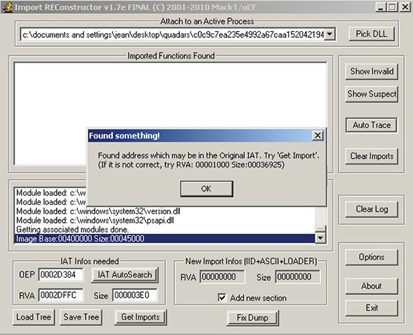
Figure 13-38 ImpREC found the OEP.
44. Click Get Imports. This will fill up the Imported Functions Found list. See whether there are invalid thunks by clicking Show Invalid. Figure 13-39 shows the output. From what is shown so far, everything looks good.
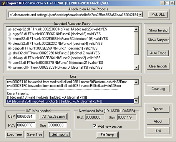
Figure 13-39 Imports found by ImpREC.
45. Once everything looks good and is completed, click Fix Dump and choose the file you dumped with LordPE. ImpREC will create a new file ending with .EXE. This is now your new unpacked binary.
46. Static analysis can now be done in this unpacked binary. You can now also disassemble and analyze it statically using IDA. Figure 13-40 shows the result in IDA.

Figure 13-40 Unpacked binary loaded in IDA.
Malcode Analyst Pack
Malcode Analyst Pack by David Zimmer is a package of utilities that helps in performing rapid malware code analysis. The package includes the following tools:
![]() Shell extensions, including the following:
Shell extensions, including the following:
![]() MD5 hash
MD5 hash
![]() Strings
Strings
![]() Query VirusTotal
Query VirusTotal
![]() Submit to VirusTotal
Submit to VirusTotal
![]() socketTool Manual TCP client for probing functionality
socketTool Manual TCP client for probing functionality
![]() MailPot Mail server capture pot
MailPot Mail server capture pot
![]() fakeDNS Spoofs DNS responses to controlled Internet Protocol (IP) addresses
fakeDNS Spoofs DNS responses to controlled Internet Protocol (IP) addresses
![]() sniff_hit HTTP, IRC, and DNS sniffer
sniff_hit HTTP, IRC, and DNS sniffer
![]() sclog Shellcode research and analysis application
sclog Shellcode research and analysis application
![]() IDCDumpFix Aids in quick RE of packed applications
IDCDumpFix Aids in quick RE of packed applications
![]() Shellcode2Exe Embeds multiple shellcode formats in EXE husk
Shellcode2Exe Embeds multiple shellcode formats in EXE husk
![]() GdiProcs Detect hidden processes
GdiProcs Detect hidden processes
![]() Finddll Scan processes for loaded DLL by name
Finddll Scan processes for loaded DLL by name
![]() Virustotal Virus reports for single and bulk hash lookups
Virustotal Virus reports for single and bulk hash lookups
You can download Malcode Analysis Pack from http://www.woodmann.com/collaborative/tools/index.php/Malcode_Analysis_Pack.
Rootkit Tools
Finding a rootkit is tricky. It takes a lot of patience to uncover one. Couple that with the right combination of tools, and a rootkit can be revealed. One of my favorite tools that helps in analyzing malware with rootkit capabilities is Rootkit Unhooker. It’s a classic tool, but it is still useful.
Some of its capabilities include the following:
![]() SSDT hooks detection and restoration
SSDT hooks detection and restoration
![]() Shadow SSDT hooks detection and restoration
Shadow SSDT hooks detection and restoration
![]() Hidden processes detection, termination, and dumping
Hidden processes detection, termination, and dumping
![]() Hidden drivers detection and dumping
Hidden drivers detection and dumping
![]() Hidden files detection, copying, and deletion
Hidden files detection, copying, and deletion
![]() Code hooks detection and restoration
Code hooks detection and restoration
You can download Rootkit Unhooker from http://www.antirootkit.com/software/RootKit-Unhooker.htm.
Rootkit Revealer is another classic rootkit tool. Unfortunately, Microsoft has discontinued it, but it can still be downloaded from different file hosting sites. Just be careful when downloading this file from non-Microsoft sources; it might come with some extra “bonus content.” But if you are adventurous, one site you can download this from is http://download.cnet.com/RootkitRevealer/3000-2248_4-10543918.html.
Network Capturing Tools
A malware’s network communication can reveal a lot about malware, the most important of which is what data is being exfiltrated out. It also reveals the malware’s network resources, such as its command and control if it is part of a botnet, its domain or IP drop zone if it is an information stealer, and its malware-serving domain or IP address if it has the capability to update itself on a regular basis. It is therefore important to capture any network communication a malware makes while it is executing in a controlled environment.
The following are the three most common network capturing tools used in malware analysis:
![]() Wireshark
Wireshark
![]() TCPDump
TCPDump
![]() TCPView
TCPView
Wireshark
Wireshark is a popular, versatile, and easy-to-use tool when it comes to capturing network traffic, as demonstrated in Lab 12-6 in the previous chapter.
You can download Wireshark from https://www.wireshark.org/.
TCPDump
TCPDump is a command-line packet analyzer tool. It is an open source tool commonly used for monitoring or sniffing network traffic. It captures and displays packet headers and everything that you need to know to understand a target file’s network communication.
You can download TCPDump from http://www.tcpdump.org/.
TCPView
TCPView is part of Sysinternals Suite. It is a tool that shows detailed listings of all Transmission Control Protocol (TCP) and User Datagram Protocol (UDP) endpoints on your system, including the local and remote addresses and the state of TCP connections.3
Lab 12-5 in the previous chapter shows how to use TCPView.
You can download TCPView from https://technet.microsoft.com/en-us/sysinternals/bb897437.aspx.
As previously stated, combining the use of different tools to solve a malware analysis problem or use case is not a foreign idea. In the previous lab, you manually unpacked a packed malware. This is a problem every malware analyst and researcher has faced, but there is one more that proves to be equally or even more of a headache than packed malware. It’s a malware with rootkit capabilities. The right combination of tools can help a malware analyst and researcher reveal the presence of a rootkit in an infected system. This is made possible if you know what to look for and how to correctly analyze a rootkit.
In this lab, you will perform a complete analysis of a user-mode rootkit using the tools discussed in this book. You will look at the different indicators of a rootkit and how to find them.
The malware that you will use specifically for this lab has the following characteristics:
![]() MD5 b4024172375dca3ab186648db191173a
MD5 b4024172375dca3ab186648db191173a
![]() SHA1 da39a3ee5e6b4b0d3255bfef95601890afd80709
SHA1 da39a3ee5e6b4b0d3255bfef95601890afd80709
![]() SHA256 e3b0c44298fc1c149afbf4c8996fb92427ae41e4649b-934ca495991b7852b855
SHA256 e3b0c44298fc1c149afbf4c8996fb92427ae41e4649b-934ca495991b7852b855
What You Need:
![]() Static analysis tools
Static analysis tools
![]() Dynamic analysis tools
Dynamic analysis tools
![]() Sysinternals Suite
Sysinternals Suite
![]() PE viewers
PE viewers
![]() Network capturing tools
Network capturing tools
![]() System running Windows
System running Windows
![]() Rootkit malware
Rootkit malware
1. You will perform basic static analysis on the file before you do anything else.
2. You start by calculating the file’s hashes. Hashes are often used as unique identifiers of files. The following are the resulting hashes:
![]() MD5 b4024172375dca3ab186648db191173a
MD5 b4024172375dca3ab186648db191173a
![]() SHA1 da39a3ee5e6b4b0d3255bfef95601890afd80709
SHA1 da39a3ee5e6b4b0d3255bfef95601890afd80709
![]() SHA256 e3b0c44298fc1c149afbf4c8996fb92427ae41e4649b-934ca495991b7852b855
SHA256 e3b0c44298fc1c149afbf4c8996fb92427ae41e4649b-934ca495991b7852b855
![]() SHA512 cf83e1357eefb8bdf1542850d66d8007d620e4050b5715dc-83f4a921d36ce9ce47d0d13c5d85f2b
SHA512 cf83e1357eefb8bdf1542850d66d8007d620e4050b5715dc-83f4a921d36ce9ce47d0d13c5d85f2b
![]() 0ff8318d2877eec2f63b931bd47417a81a538327af927da3e
0ff8318d2877eec2f63b931bd47417a81a538327af927da3e
![]() SSDeep 12288:tcJkcAWoVBMRLuDHt9pH4jZ/6v5hLl4sk8rEvCV1MK SK:gTr+OpuDH8N4Xw8AKfnSK
SSDeep 12288:tcJkcAWoVBMRLuDHt9pH4jZ/6v5hLl4sk8rEvCV1MK SK:gTr+OpuDH8N4Xw8AKfnSK
![]() ImpHash ef471c0edf1877cd5a881a6a8bf647b9
ImpHash ef471c0edf1877cd5a881a6a8bf647b9
MD5 has been an industry standard for a long time, but because of MD5 collisions, it is always better to get more hashes. ImpHash is a relatively new hash that was created from the import table rather than the raw data of the file. ImpHash is only for PE files.
3. Aside from hashes serving as unique identifiers, it will also allow you to look for this sample in publicly available malware databases such as VirusTotal and even look at publicly available sandboxes to see whether it has been analyzed already. Remember that all the information you get helps you in analyzing malware, especially if you are struggling.
4. Check the file type. Usually, when you get a sample, it is always assumed that it is a PE file, but this is not always the case. Also, using the different file type checkers in your arsenal such as PEiD and a Python script powered with Yara will help you identify not only the file type but also whether the file is packed, encrypted, or neither.
5. For this file, you will use the easiest way to determine the file type. You will use GNU file command.

The output tells you that this file is UPX compressed. You will find out later if it is indeed UPX compressed.
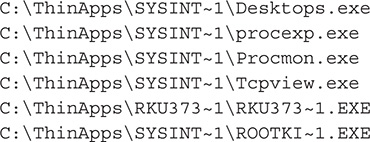
6. Get the strings present in the file. You can do this by using the GNU command strings or SysInternals strings.exe in Windows. Here is a partial list of the strings found in the file:

7. From the strings output, notice the following strings: UPX0, UPX1, UPX!, and AutoIt. The first three are indicators that the file is packed by UPX, and the fourth string indicates that there might be an AutoIt script embedded in the file, which might be a second packer.
8. Investigate the file’s PE characteristics. You can do this using PEView. Figure 13-41 shows the file’s compile time. The compile time is found inside the PE structure as a member called TimeDateStamp in the NT headers. The compile time value should be taken into limited consideration because this value can be faked easily.
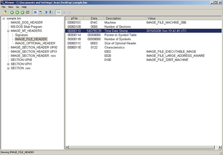
Figure 13-41 PEView showing the compile time of the file.
9. Figure 13-42 shows the file’s machine value. The machine value is a member in the NT headers structure, and it can have one of two values: 0x014C, which indicates a 32-bit Windows PE file, or 0x8664, which indicates a 64-bit Windows PE file.

Figure 13-42 PEView showing the file’s machine value.
10. Looking at the PEView windows, it is easy to notice one section name. Sometimes the PE section name can give you some information about the file. In this example, the PE section names that can be seen are UPX0, UPX1, and .rsrc, as shown in Figure 13-43. UPX0 and UPX1 indicate that the file has been packed with UPX. PEView is the third tool that confirms the file is packed with UPX. The first two are the GNU file and strings command line.

Figure 13-43 PEView showing UPX section.
11. The section named .rsrc suggests that the file contains a resource section. This is a good place to extract some useful information. For this purpose, you will use Resource Hacker, which allows you to look at the resources embedded into the binary, as shown in Figure 13-44. Notice the suspicious little resource SCRIPT that is under RCDATA. This may be the AutoIt script in an encrypted format.
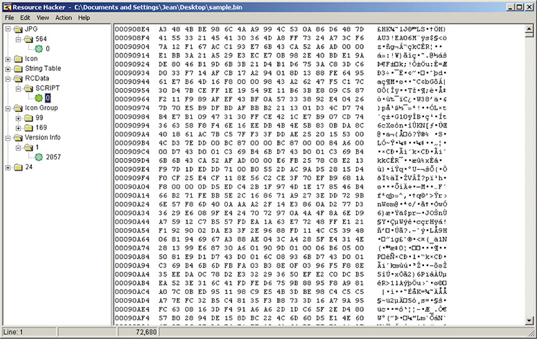
Figure 13-44 Resource Hacker view of .rsrc.
12. Get Imports/Exports information. A great tool for this specific purpose is Dependency Walker. This tool shows all the libraries imported by the binary and which functions are imported from each library (green) as well as all the exported functions of each library and the binary, if any. Figure 13-45 shows this.

Figure 13-45 Dependency Walker.
13. Some of the information including the MD5 hash, strings, size, and compile time can be collected using Malcode Analyst Pack. This also enables you to submit the file to VirusTotal or simply run a query to check whether security products already detect the file.
14. You can now proceed to dynamic analysis. You will be using a clean malware analysis system that you built from previous labs. For this example, you will be using a virtual machine.
15. Run Process Explorer, Process Monitor, and TCPView in the malware analysis system (guest OS) or sandbox. Doing this will start their monitoring functionality.
Having these tools run in clean systems makes you familiar with the output of these tools in a clean system, which is good for baselining. Doing this will give you experience spotting something out of the ordinary in case you are using these tools to determine a possible infection and not for analyzing a specific malware sample.
16. Run Wireshark in promiscuous mode on the host OS. Make sure you are capturing communication traffic on the network adapter that the VM is connected to. In this lab, the name of the interface is vmnet8.
17. Once everything is set, run the malware sample.
18. Watch closely and take notes on both TCPView’s and Process Explorer’s windows. In Process Explorer, look for any new processes/children exiting and dying. New sessions/processes are green, and those that are killed are red. In TCPView, look for any network sessions being created and dropped. See Figures 13-46, 13-47, and 13-48.
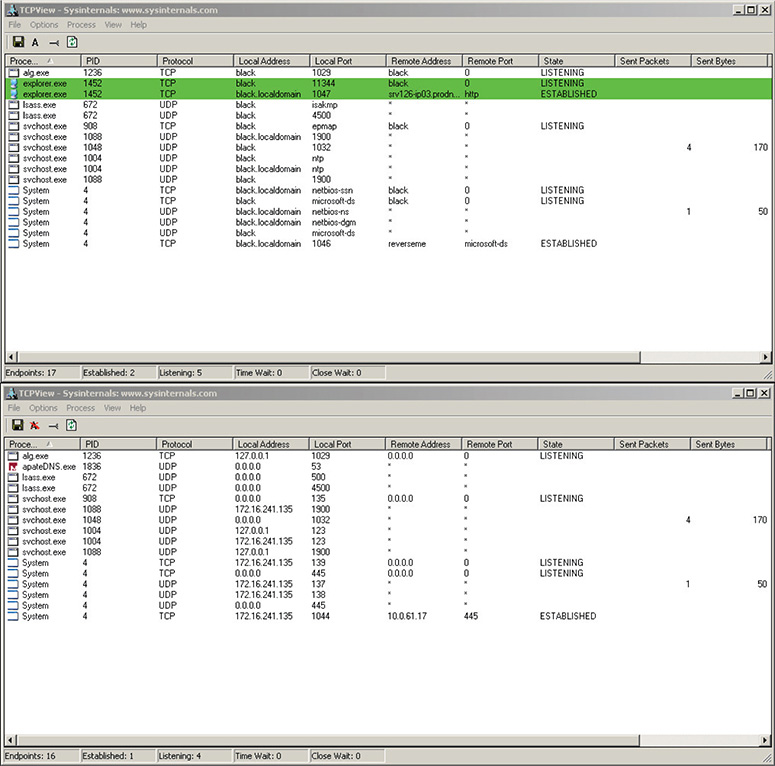
Figure 13-46 Two instances of TCPView output.
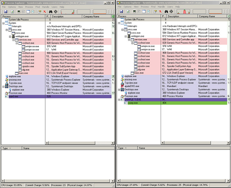
Figure 13-47 Two instances of Process Explorer output.

Figure 13-48 Two instances of Process Monitor output.
19. Take notes of all these traces. It will give you some insight later during analysis.
20. Check out the output of Wireshark running in the host OS. Figure 13-49 shows this.
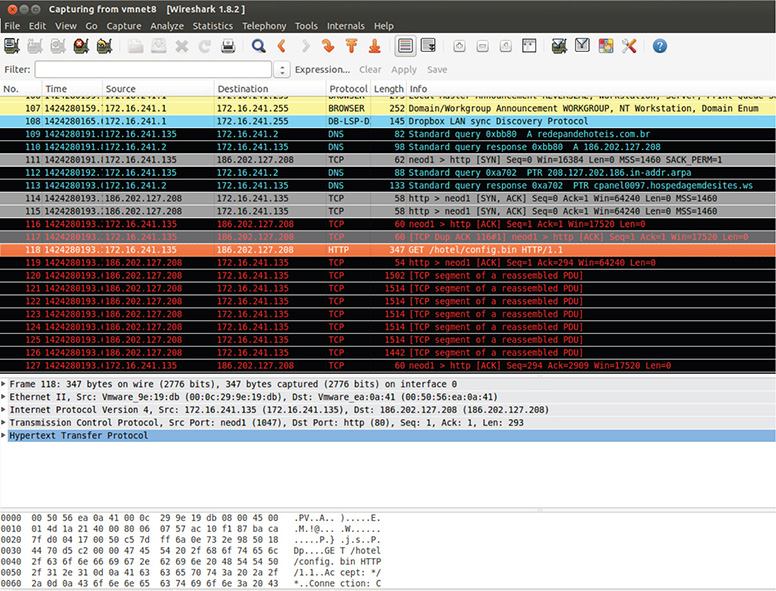
Figure 13-49 Wireshark output.
21. Let the sample run for a few minutes.
22. After letting the sample run for a few minutes, stop the captures on both Process Monitor and Wireshark. Save the capture log from Process Monitor and save the pcap capture from Wireshark.
24. Let’s analyze the pcap capture from Wireshark. You should be able to see a few Domain Name System (DNS) queries followed by an HTTP GET request downloading a file called config.bin, as shown in Figure 13-50. Take note of the filter.

Figure 13-50 HTTP GET request in Wireshark.
25. Follow the TCP stream of the HTTP GET request. Figure 13-51 shows the result. Take note of the address redepandehoteis.com.br/hotel/config.bin. You got redepandehoteis.com from the Host section and /hotel/config.bin from the GET request.

Figure 13-51 HTTP GET TCP stream.
26. Next you see a few HTTP POST requests to the same server, as shown in Figure 13-52. Take note of the address redepandehoteis.com.br/hotel/gate.php.
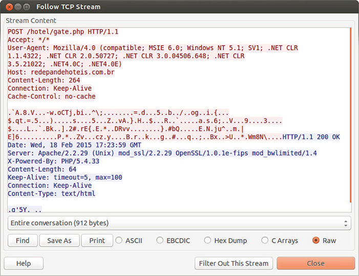
Figure 13-52 HTTP POST TCP stream.
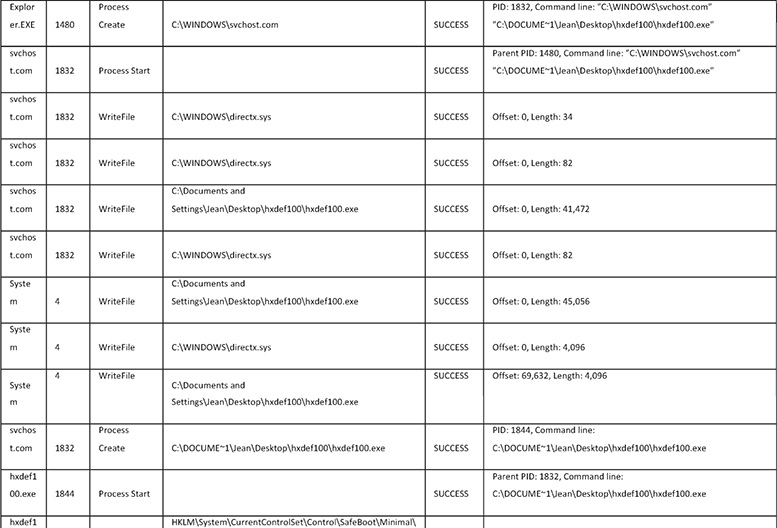
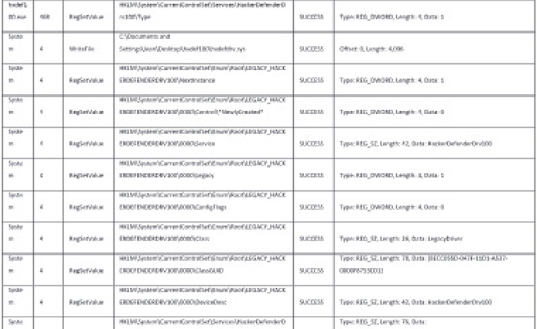
27. Let’s go to the capture log from Process Monitor. Process Monitor captures the file’s activity in the following: processes, the registry, and files. For the purpose of this lab, you will group the file activities by deployment process, persistency mechanism, browser settings, and malicious activity. This means you will identify which of the malware activities in the processes, the registry, and files have contributed to the deployment process, persistency mechanism, browser settings, and malicious activity.
The following are the tables for the deployment process.
Here is the table for processes:


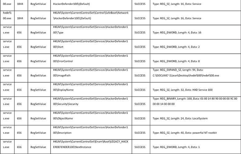
The following tables relate to the persistency mechanism.
Here is the table for the registry:
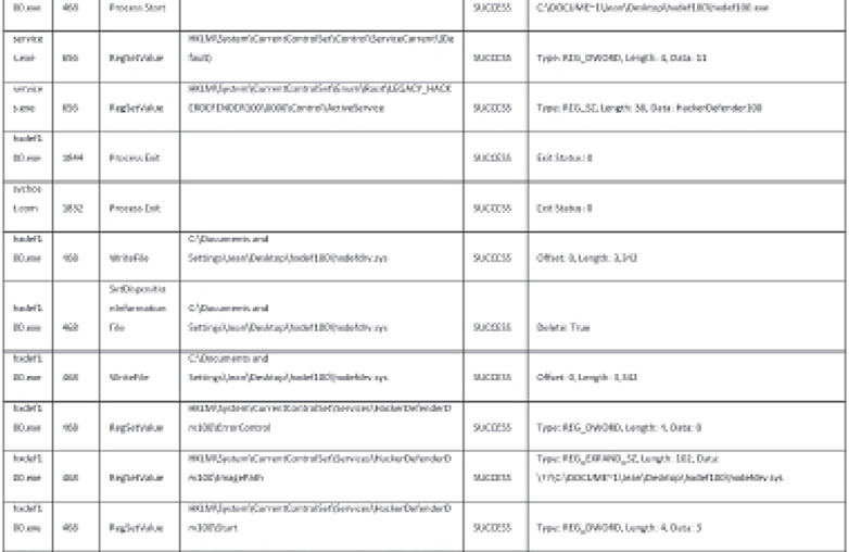
Here is the table for the files:
![]()
The following tables relate to browser settings.
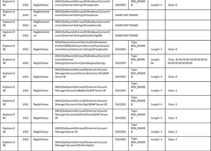
Here is the table for the registry:


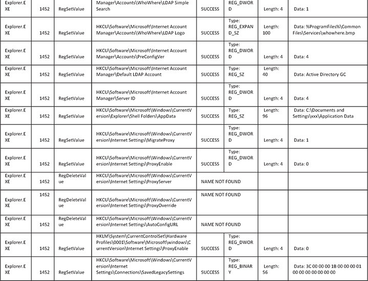
Here is the table for the files:
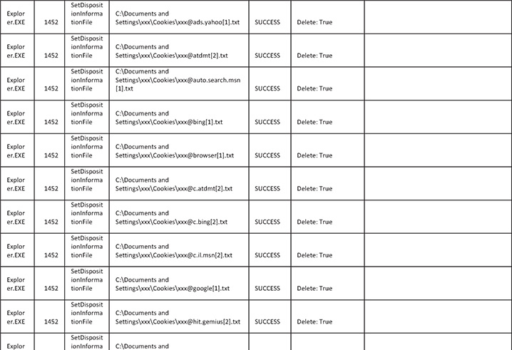
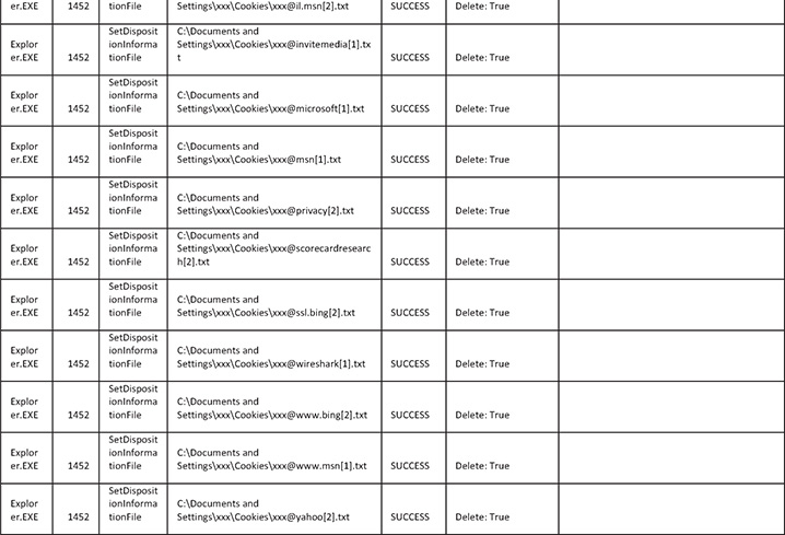
Here is the malicious activity for files:
![]()
28. Regarding browser settings, from the logs you can see that the malware is overwriting a lot of the system’s browser settings as well as deleting cookies and proxy settings. The reason for this is that the malware does not want any interference with its operation and is eliminating potential interferences by doing that. Another reason for cookie deletion and emptying different caches is that the malware wants the user to log in to websites so the credentials can be stolen.
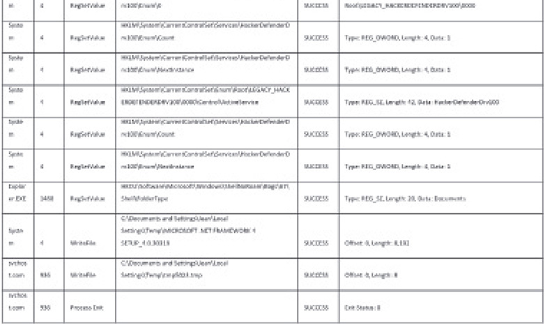
29. Regarding deployment, the logs reveal that the malware copies itself to the C:Documents and Settings folder and eventually runs a batch file that creates and runs qyecy.EXE.
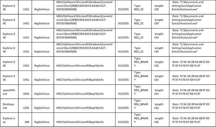
30. Regarding the persistency mechanism, the malware creates a registry key under HKCUSoftwareMicrosoftWindowsCurrentVersionRun, which is a known registry location to execute files during startup. The key name is {9EBEC959-DCC9-EA18-5427-D5C9258D0AD8}, and it contains the path to the malware’s file location, which is C:Documents and Settingsxxx Application DataUlkuasoul.exe.
31. Also notice that the following registry event repeats itself every few seconds. This will re-create the malware’s persistency in case someone intentionally deletes it. The malware also saves some encrypted configuration data at HKCUSoftwareMicrosoftRupeKatifa.
![]()
32. Regarding malicious activity, at first glance it might seem that the file C: Windowsdirectx.sys dropped by the malware is a driver and that the malware has kernel mode capabilities, but this is not the case. The filename was carefully picked in order for it to blend in with the rest of the files in that folder. If you look at the contents of the file, you will see clear text separated by newline characters.
This file is where the malware keeps a list of currently running processes.
33. You may have noticed that most suspicious registry events were initiated by a process named Explorer.EXE, which was running even before you ran the malware on the machine and is actually a legitimate Windows process that is responsible for Windows’ graphical user interface (GUI) environment. Also, you may have noticed that some suspicious events happened more than once and were sometimes initiated by a few different processes that are also legitimate and were running before you infected the machine. The simple explanation for this is that this malware is creating a thread that runs the malware inside all processes that are already running on the machine. This process is called code injection or thread injection. When malware is injecting itself into a process, it is doing it to hide its process from showing when process listing occurs. This technique is usually utilized by a user mode rootkit.
34. Aside from code injection, another technique that is commonly used by user mode rootkits is hooking. User mode hooks are implemented in many creative ways; the most common techniques are IAT modification and inline patching.
In IAT modification, the malware changes the IAT of each binary that is loaded by the OS in memory and changes the imported libraries and functions to their own malicious version of the same library containing the same functions with “extra functionality.”
With inline patching, the malware will patch the code of the library in memory in a way that prior to the execution of the function, it will jump to the malware’s code, and after executing the malicious code, it will jump back to the original function and continue with the original function’s execution flow.
Both methods will not be detected by checking whether any of the operating system’s file integrity was compromised because the malware is doing all its work in memory. As a result, no traces will be found in the original files in the file system.
NOTE
Hooking techniques such as IAT modification and inline patching are also used by legitimate applications/programs; therefore, the existence of hooks does not necessarily mean that the machine is infected with malware.
35. To check for hooks, you will scan the machine using Rootkit Unhooker. At this point, you should resume the VM and run Rootkit Unhooker. To scan for user mode hooks, go to the Code Hooks tab and click the Scan button. If there are code hooks on the infected system, it should look like Figure 13-53.

Figure 13-53 Rootkit Unhooker output.
36. Save the output by going to the Report tab and clicking the Scan button. Uncheck all boxes except Code Hooks and click OK. Once the report is done, copy the text and save it to a file.
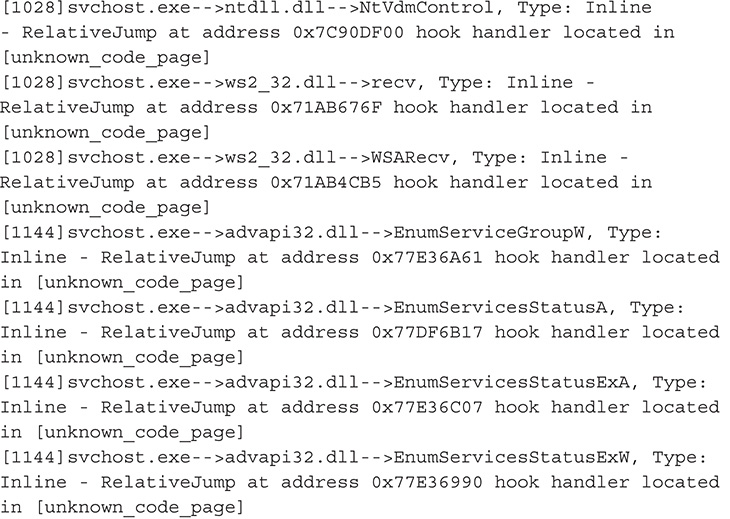
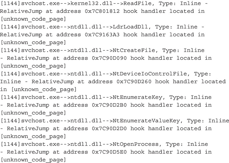
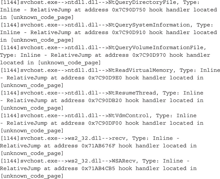
37. The complete output with the result is shown here:

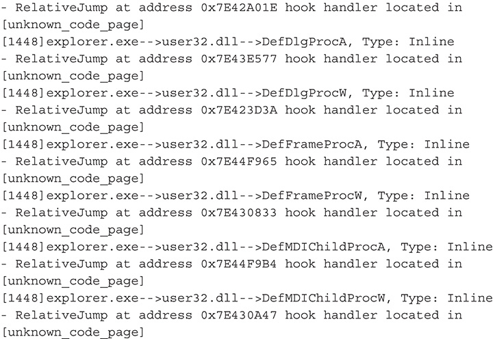
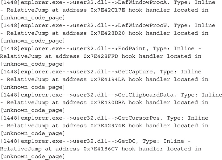
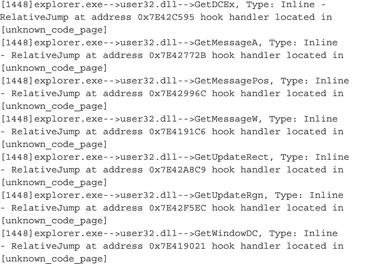
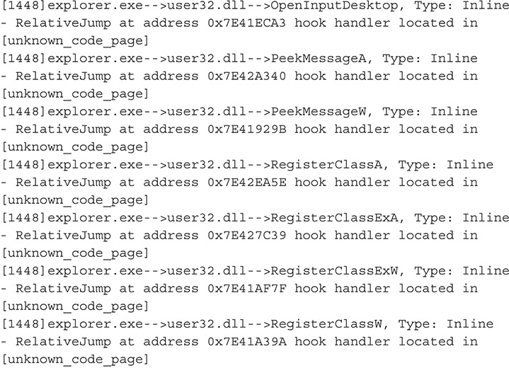


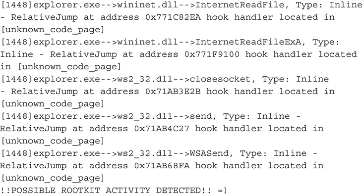
38. From this output, you can definitely say that you are dealing with a user mode rootkit. Also based on this output, this malware hooks functions in wininet.DLL and ws2_32.dll, which are libraries that deal with network communications and Hypertext Transfer Protocol (HTTP). By hooking functions in these libraries, the malware may be able to tamper with network traffic and set up a man-in-the-middle attack.
39. Next is dump analysis. This is done by taking a memory dump of the malicious process. In this case, the malware injected itself into each one of the running processes, with Explorer.EXE being the most significant. You will therefore pick Explorer.EXE as your memory dump’s target. You can use either Process Explorer or Rootkit Unhooker to take a memory dump.
40. Dump a process with Process Explorer. Right-click the target process, which is Explorer.EXE, and go to Create Dump | Create Full Dump; then save the dump file. You can name the file MEMORY.DMP. See Figure 13-54.

Figure 13-54 Taking a memory dump using Process Explorer.
41. Dump a process with Rootkit Unhooker. Go to the Processes tab. Right-click the target process, which is Explorer.EXE. Click Dump All Process Memory and save to a file. You can name the file MEMORY.DMP. See Figure 13-55.

Figure 13-55 Taking a memory dump using Rootkit Unhooker.
42. Once you have the memory dump, you can proceed to analyze it using the different tools you have in your disposal. A basic analysis can start with the strings GNU command line or Sysinternals Strings.EXE.
43. In this lab, you will use the GNU strings command line and save the file to a text file named memory_dmp_strings.txt.
![]()
TIP
The output of strings is really huge; it’s always a good idea to redirect the output to a file and review it with a text editor.
44. The following is the output from strings:

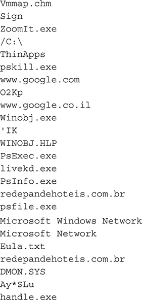
45. Grep for specific patterns such as http. You can do this together with strings by using a pipe.
![]()
46. The following is the output:

47. Notice the last three from the output; these strings are part of the config file that was downloaded at the beginning of the malware’s execution.
48. What you have done is a basic dump analysis. There is a more advanced way of doing this. For this purpose, you will use the Volatility framework. As previously discussed, Volatility is a Python-based framework that allows a user to analyze the OS environment from a static dump file. It has many plug-ins that are useful when it comes to memory analysis. You can find a list of its basic plug-ins in Appendix C.
Volatility analyzes .VMEM files created by VMware. Volatility also supports other virtualization products such as VirtualBox.
To get started, you need to suspend the VM prior to analyzing the .VMEM.
49. Once the VM is suspended, copy the .VMEM file to your working folder. Let’s assume your .VMEM file is Sandbox.VMEM.
50. Find API hooks (user mode hooks) using Volatility. For this purpose, you will use the apihooks plug-in.
![]()
51. The following is the output:
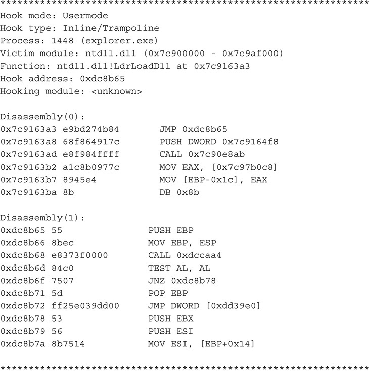

52. As shown in the output, the plug-in shows you each function that is hooked, what type of hook is used, and the original code versus the tampered code.
53. Find arbitrary malicious pieces of code. To do this, you will use the malfind plug-in, which allows you to find where exactly in a process memory the malware’s injected code is.
![]()
54. The following is the output:
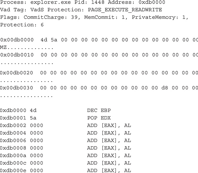
55. As shown in the output, the plug-in shows you the injected malware in the process Explorer.EXE.
56. Feel free to experiment some more on the different plug-ins offered by Volatility to see whether you can gather more information from the .VMEM file that will help you paint a clearer picture of the malware.
57. Once you have all the information you need from the tools discussed in this lab, you can write a detailed report about the rootkit capability of this malware.
In this lab, you will perform a complete analysis of a kernel mode rootkit using the tools discussed in this book. The sample used for this lab is Hacker Defender version 1.00.
What You Need:
![]() Static analysis tools
Static analysis tools
![]() Dynamic analysis tools
Dynamic analysis tools
![]() Sysinternals Suite
Sysinternals Suite
![]() PE viewers
PE viewers
![]() Network capturing tools
Network capturing tools
![]() OSR driver loader
OSR driver loader
![]() System running Windows
System running Windows
![]() Rootkit malware
Rootkit malware
Steps:
1. You begin with basic dynamic analysis of the sample by running it in a virtual environment malware analysis system and monitoring all processes, the registry, and the file system by using the techniques discussed in Lab 13-7. Take note that the username of the analysis system is Jean, so you will see this in the output of the tools and some screenshots in this lab.
2. After infecting the VM, you monitor the following events in Process Monitor.

3. The following are some things that are noticeable in the dynamic analysis session:
![]() A file named hexdefdrv.sys was written in C:Documents and Settings<User>Desktophxdef100.
A file named hexdefdrv.sys was written in C:Documents and Settings<User>Desktophxdef100.
![]() A service named HackerDefender100 was created by writing values to the registry.
A service named HackerDefender100 was created by writing values to the registry.
This tells you that the malware is possibly installed as a kernel mode driver on the system, which is used to gain kernel rootkit capabilities.
4. Notice that all the files related to the malware have vanished. In Figure 13-56, you can see that the listed directory in the File Explorer doesn’t actually exist on the desktop.
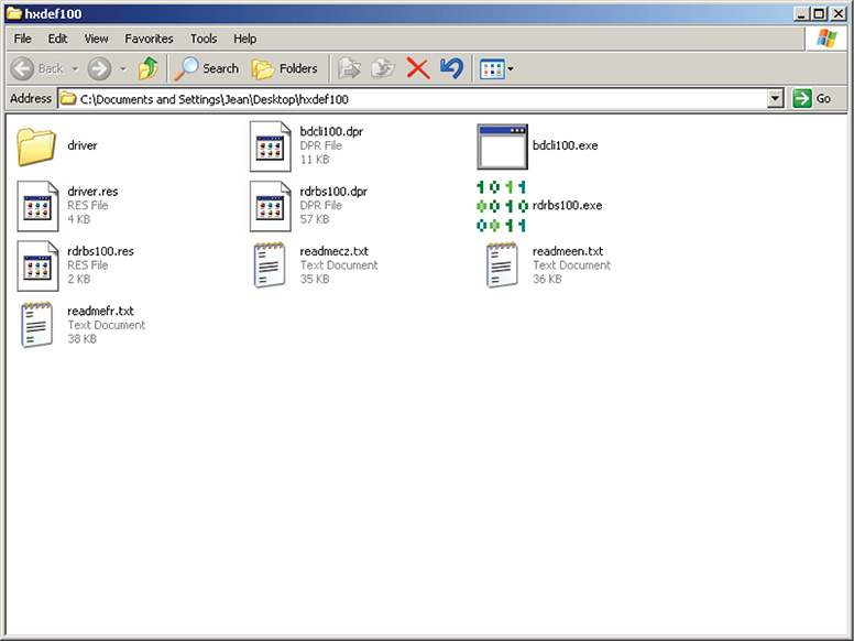
Figure 13-56 File listing of hxdef100.
5. When you try to find the newly installed service in the Services snap-in by going to Run, typing services.msc, and clicking Enter, you will not be able to find it in the listing, as shown in Figure 13-57.
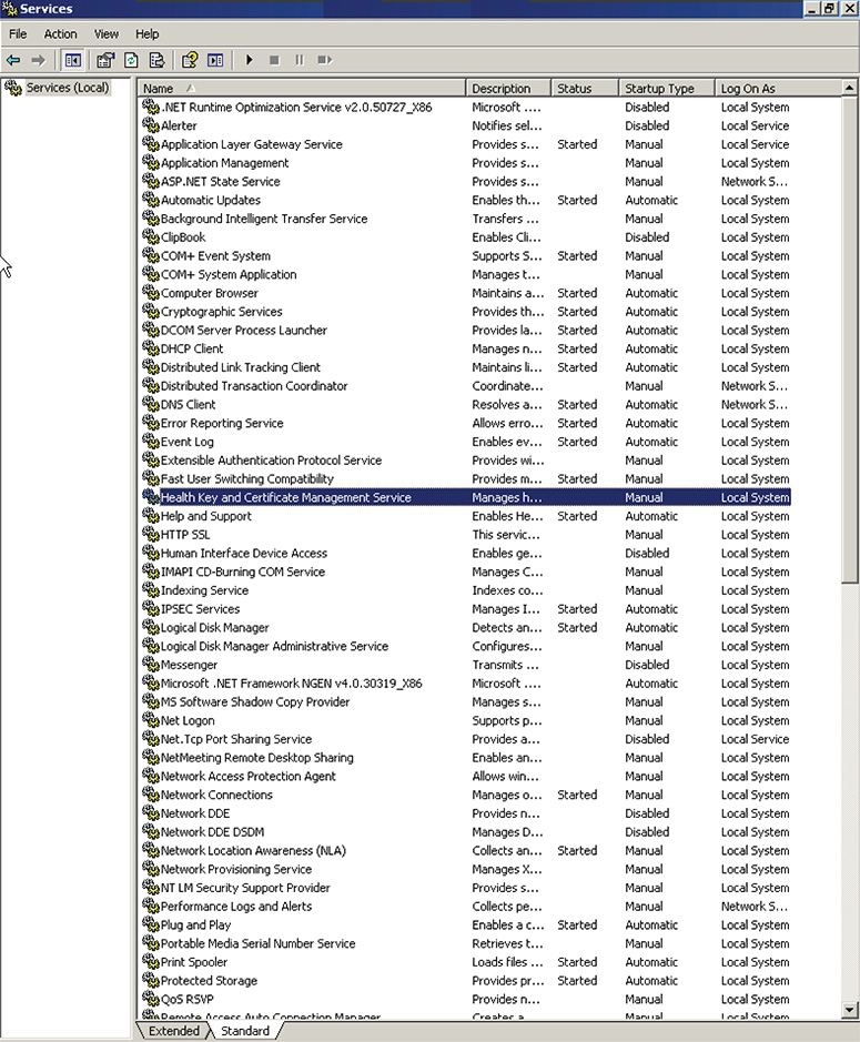
Figure 13-57 Running services in the local machine.
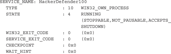
6. Another way to check the service status and parameters is through the command line by running the following command:
![]()
7. In this case, you want to check about a service named HackerDefender100. You know this through the output of Process Monitor.
![]()
8. The following output reveals that the service exists, but it is hidden from any user mode application that tries to list the system’s services:
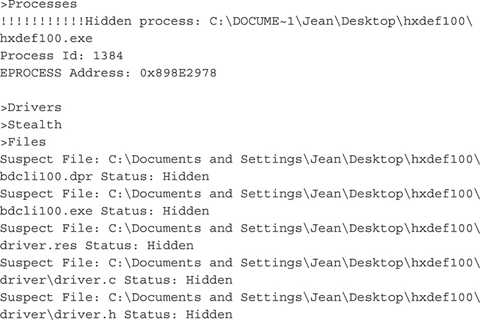
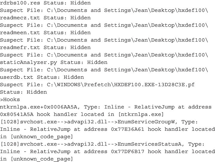
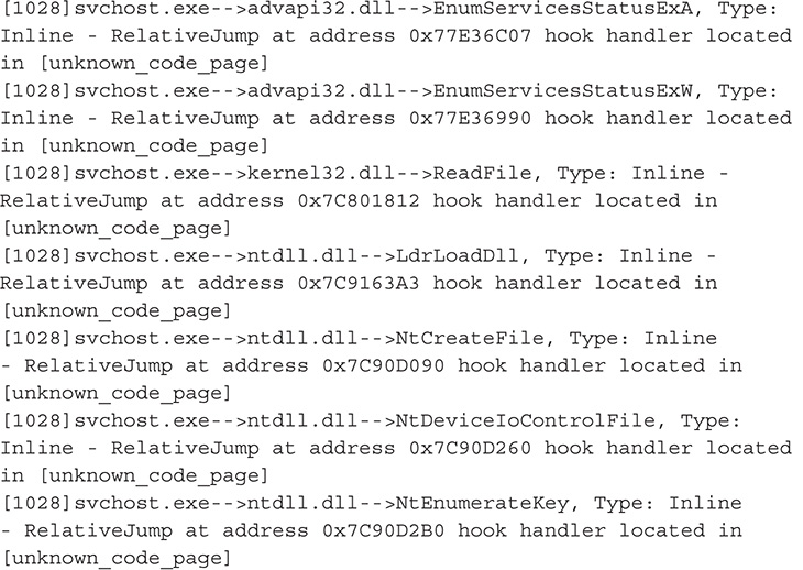
9. A scan with Rootkit Revealer should confirm these suspicions.
10. Here is the rootkit revealer output:


11. After your initial analysis, you should have a picture of what kind of malware you are dealing with. You know that it installs a driver and that it hides certain files. You should now try to analyze the driver itself.
12. At this point, you should revert the machine to its original state before the infection so you can use a kernel debugger to see what the driver is actually doing and to extract the driver’s files.
TIP
It is always wise to save a snapshot of your dynamic analysis session so you can come back to it when needed without going through the whole process of infection again.
13. Let’s set up your debugger and debuggee machine. The debugger machine is where WinDbg will be, and the debuggee machine is where the malware will run. This can be the VM you just reverted to its original state. Both these machines are virtual environments. You will set up the environment using VMware hosted on a Linux machine.
14. The first VM, which is the debuggee or debugged machine, is running Windows XP SP3. As mentioned, this is where you will run the malware. The second VM, which is the debugger machine, is running Windows 7 (XP can also be used). As mentioned, this machine will run WinDbg attached to the other VM via the serial port (COM port).
15. The first thing you have to do is add a serial port to both VMs. This is the medium to form a link between the debugger running on the debugger machine to the debuggee or debugged machine. The next steps of adding a serial port must be done for both VMs.
16. To add a serial port, turn off the virtual machine; then go to Virtual Machine Settings, as shown in Figure 13-58.
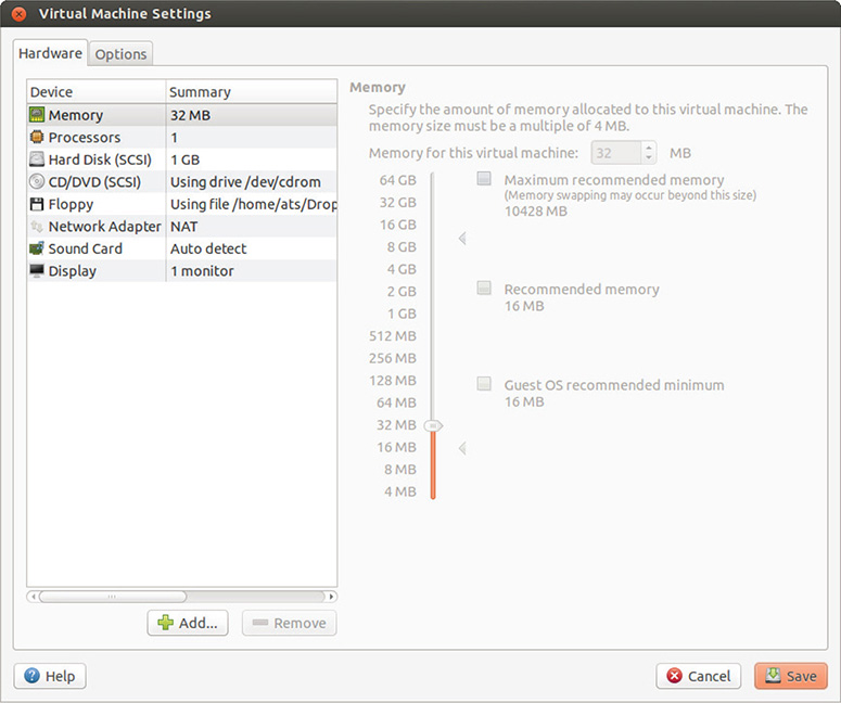
Figure 13-58 VMWare Virtual Machine Settings.
17. Click + Add, choose Serial Port, and click Next, as shown in Figure 13-59.

Figure 13-59 VMWare Add Hardware Wizard.
18. Choose Output To Socket and then click Next, as shown in Figure 13-60.

Figure 13-60 Serial Port Type.
19. Since you are using a Linux host, the following applies. On both machines, enter the socket name /tmp/<socket>. <socket> should be replaced with a short string (for instance, debugport0) and should be the same on both virtual machines.
20. On the debugged VM or debuggee, set From to Server and set To to A Virtual Machine, as shown in Figure 13-61.

Figure 13-61 From server to a virtual machine.
21. On the debugger VM, set From to Client and set To to A Virtual Machine, as shown in Figure 13-62.
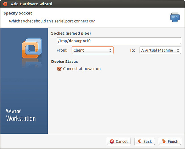
Figure 13-62 From client to a virtual machine.
22. Just in case you want to use a Windows machine to host the two virtual machines, the process is the same except for the Socket (Named Pipe) path. It should follow the Windows path and should look like this: \. pipe<namedpipe>.
23. After creating the serial ports on both machines, the next step is to boot into Windows in Debug mode on the debuggee.
24. To boot Windows in Debug mode, edit the Boot.INI file located in C:. This is usually the case unless your boot partition is in another drive.
25. Start the debuggee and open Boot.INI using a text editor.
26. Assuming you have only one OS installed on your VM, the default should look like the following:

27. Add a second line under [operating systems]. The second line is the same as the first line plus the parameters for debugging. The resulting Boot.INI file should look like the following:
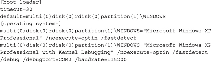
28. Pay attention to the /debugport=COM? and replace it with the right COM port number for the serial port you added earlier to the debugged machine. In the setup used to create this lab, it is COM2.
29. Reboot the debugee and use the second option in the BootLoader: Microsoft Windows XP Professional With Kernel Debugging.
30. Once this is done, you can run WinDbg on the debugger machine. But before you attach to the debugee, you need to configure the symbols in WinDbg.
31. Choose File | Symbol File Path or simply press CTRL+S. Set the search path to SRV*<your_symbol_path>*http://msdl.microsoft.com/download/symbols. The <your_symbol_path> should be replaced in your VM with the path to your symbols. In the VM you used to make this lab, it is C: WebSymbols.
32. Attach to the debuggee. Choose File | Kernel Debug or simply press CTRL+K.
33. Set the baud rate to 115200 and set the COM port to the same port number as configured for the debugger machine, as shown in Figure 13-63. Then click OK. You are now ready to do some kernel debugging.
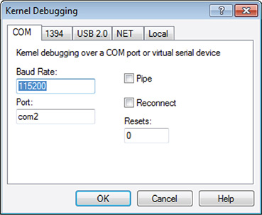
Figure 13-63 Kernel Debugging COM tab.
34. After clicking the OK button, you should get the screen shown in Figure 13-64.
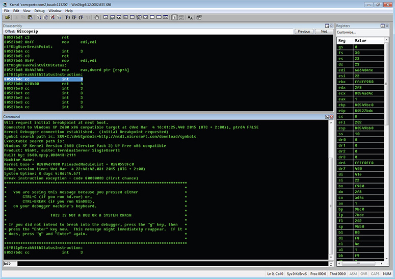
Figure 13-64 Debugging window.
35. In case your screen keeps saying “Debuggee not connected” at the bottom left, you can try to remedy this by choosing Debug | Kernel Connection | Resynchronize or by pressing CTRL+ALT+B and waiting for a few seconds. If this does not help, check the machine configurations and check whether you got all the COM port numbers right.
36. Once a connection is established successfully, you can proceed.
37. At this point, you established the connection to the debuggee and broke into a random address in the OS code. This is irrelevant for your analysis. This is a side effect of you breaking into the debugged machine. There is unresponsiveness to any input/output (I/O) operation until you continue the execution of the OS code.
38. Before you continue the execution of the OS and infect the machine, choose Debug | Event Filters and then set the Load module to enabled and handled, as shown in Figure 13-65.
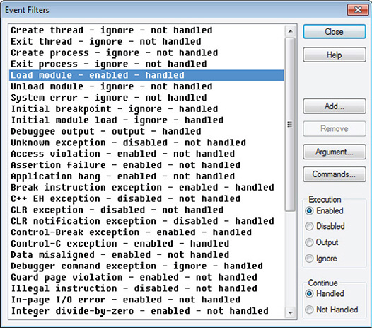
Figure 13-65 Event filters.
39. Since you need some interaction with the debugged machine in order to infect the machine prior to your analysis, you will continue the execution by pressing F5 or typing g (an abbreviation for go) and pressing Enter at the WinDbg command prompt.
![]()
40. After continuing the execution, WinDbg should show “Debuggee is running…” on the console line.
41. At this point, you should infect the debugged machine by running the malware. This time you will break once the driver module is loaded. Figure 13-66 shows what the WinDbg window should look like once you break into DriverEntry.

Figure 13-66 Breaking into DriverEntry.
42. Typing lmf at the command prompt reveals that the driver module was loaded successfully, as shown in Figure 13-67.

Figure 13-67 Rootkit driver loaded.
43. Type dd $iment(hxdefdrv) to check the driver’s entry point and then put a breakpoint in that address by typing bp <entry_point_address>. In the current setup when this lab was being created, the address is 0xBAFA3718.
44. Continue the execution by pressing F5 or typing g in the console until you hit the driver’s entry point. Figure 13-68 shows the whole session.
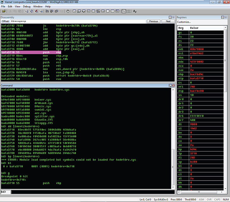
Figure 13-68 Revealing the driver’s entry point.
45. Once you hit the driver’s entry point, you can start debugging it to see how it works by using the Step Over (F10) and Step Into (F11) functions. But it would be easier to dump the driver’s module and analyze it with IDA first.
46. To do this, you create a snapshot of the debugged machine so you can continue debugging later with WinDbg, and then you pause the virtual machine.
47. Use Volatility to see some of the kernel structures and dump the driver file. Refer to the previous Lab 13-7 for more information on using Volatility for this purpose.
48. You’ll start with checking the loaded modules, which includes drivers, by running the following command:
![]()
49. Among the list of modules produced, you can see your suspicious hxdefdrv. sys module, which is loaded in the address 0xBAFA300. Take note that this address might be different in your own experiment.
![]()
50. Now you can dump all of the loaded modules along with your malicious driver by running the following command, as shown in Figure 13-69:
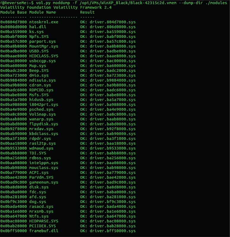
Figure 13-69 Volatility moddump results.
![]()
51. You should now have a directory full of .sys files in this format: driver.<address>.sys.
52. Since your driver was loaded in 0xBAFA3000, you should look for driver. bafa3000.sys.
NOTE
Another thing that can be interesting is checking for any SSDT hooks by running vol.py ssdt –f <.vmem_path>. You did not do it for this lab because this specific malware is not using SSDT hooking.
53. Now you can take the dumped file and feed it in IDA for analysis.
54. Once it is loaded in IDA, you should land on DriverEntry, as shown in Figure 13-70.

Figure 13-70 Dumped file loaded in IDA.
55. After analyzing the code, you should also find the DriverUnload function, as shown in Figure 13-71.

Figure 13-71 DriverUnload function revealed.
56. Eventually, you will arrive at the function that contains the main functionality of the malware, as shown in Figure 13-72.
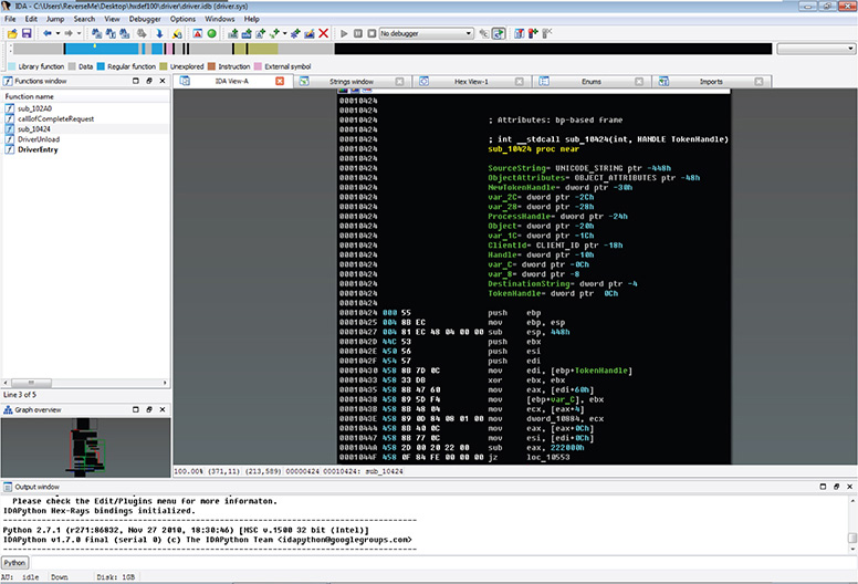
Figure 13-72 Main malicious functionality revealed.
57. Analysis of kernel mode rootkits requires familiarity with the kernel mode API. If you are not familiar with kernel mode API calls, please consult Microsoft TechNet and see the available documentation. Google is also your friend. The basic idea is that every Win32 API function encapsulates a kernel mode function and basically switches to kernel mode and calls the appropriate kernel mode function with the correct parameters.
58. After you are done with the dynamic analysis of the driver’s sys file, you can go back to the infected machine and keep debugging it by resuming the VM. Once the VM is running again, you can see the installed driver by continuing execution in WinDbg (F5 or typing g) and breaking again (CTRL+BREAK) after about 10 seconds and then pausing the machine again.
59. Now you can use Volatility again to analyze the VM’s kernel for Interrupt Request Procedure (IRP) drivers by running the following command. Figure 13-73 shows the result.
![]()
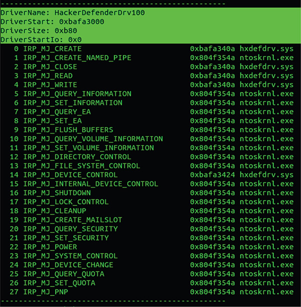
Figure 13-73 Volatility revealing IRP.
60. This reveals to you the driver’s IRP chain.
61. You have just analyzed a kernel mode rootkit.
62. Please feel free to experiment further with WinDbg. WinDbg allows you to investigate a lot of Windows structures. You can learn more about this in Microsoft TechNet and by Googling.
63. To continue your learning and to get a deeper level of understanding of rootkits and other techniques, please research further about the Windows kernel and Windows driver development.
Automated Sandboxes
In previous chapters, I discussed how to build your own malware analysis system. In this section, you will delve more into making an automated malware analysis system.
There are lots of automated sandboxes available. Some of them are software based, and some are hardware based. Some are free, while some cost a lot of money.
When it comes to open source automated sandboxes, my personal favorite is Cuckoo. It is completely open source, which means that aside from looking at its internals, you can modify and customize it as you want. Plus, you can use the skills you have learned in previous chapters to create the guest OS that will run the malware.
When Cuckoo processes a binary, it produces the following output:4
![]() Native functions and Windows API call traces
Native functions and Windows API call traces
![]() Copies of files created and deleted from the file system
Copies of files created and deleted from the file system
![]() Dump of the memory of the selected process
Dump of the memory of the selected process
![]() Full memory dump of the analysis machine
Full memory dump of the analysis machine
![]() Screenshots of the desktop during the execution of the malware analysis
Screenshots of the desktop during the execution of the malware analysis
![]() Network dump generated by the machine used for analysis
Network dump generated by the machine used for analysis
These outputs can be presented in the following formats to make it more consumable to end users:
![]() JavaScript Object Notation (JSON) report
JavaScript Object Notation (JSON) report
![]() Hypertext Markup Language (HTML) report
Hypertext Markup Language (HTML) report
![]() Malware Attribute Enumeration and Characterization (MAEC) report
Malware Attribute Enumeration and Characterization (MAEC) report
![]() MongoDB interface
MongoDB interface
![]() HPFeeds interface
HPFeeds interface
You can learn more about Cuckoo at http://www.cuckoosandbox.org/.
In this lab, you will install and configure Cuckoo 1.1 on a host running Ubuntu 14.04 LTS. It will also explain the process of installing a Cuckoo agent on a guest virtual machine running Windows XP with Service Pack 3.
This lab is divided into the following major steps:
1. Preparing the host
2. Installing Cuckoo
3. Preparing the guest
4. Installing the agent
5. Configuring Cuckoo
6. Running Cuckoo
What You Need:
![]() System running Ubuntu 14.04
System running Ubuntu 14.04
![]() Windows XP with SP3 virtual machine (you will be using VirtualBox as your virtualization software)
Windows XP with SP3 virtual machine (you will be using VirtualBox as your virtualization software)
Steps:
1. Prepare the host.
A. Install Python on your Ubuntu machine. This is necessary because all the components of Cuckoo are written in Python.
![]()
B. Install mongodb. This is needed to use the web interface.
![]()
C. Install SQLAlchemy and Python BSON packages.
![]()
D. Some dependencies used by modules and utilities within Cuckoo are optional, but their installation is recommended. For an explanation of the role of those dependencies, please refer to the requirements section of the Cuckoo sandbox documentation located at http://docs.cuckoosandbox.org/en/latest/installation/host/requirements/.

E. Install Yara by following Lab 13-1.
F. To add fuzzy hashing capabilities to your sandbox, first you need to download and install ssdeep. Get the latest source from http://ssdeep.sourceforge.net/. As of this writing, the latest version is ssdeep-2.12.
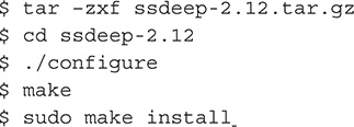
G. Download and install pydeep. Get the latest source from https://github.com/kbandla/pydeep/archive/master.zip._

H. If you encounter an error while building pydeep, make sure to install the necessary libraries for python-dev using the following command:
![]()
I. A network sniffer such as tcpdump is necessary to capture the network traffic while malware is running.
![]()
J. Set Linux capabilities to tcpdump to avoid running it as root.
![]()
A. Start by creating a new user dedicated to your sandbox. Make sure to add the new user to the group of users running VirtualBox. In this lab, you will make the user cuckoo and the group vboxusers.
![]()
B. Add the new user to the list of sudoers on the host. The visudo tool lets you edit the /etc/sudoers file.
![]()
C. Once the sudoers file is opened, add the following line at the end:
![]()
D. Save your changes to /etc/sudoers and quit.
E. Log out and then log in as the newly created user. This is important because the guest VM has to be created under the new user account so the sandbox can have access to it.
F. After logging in, extract Cuckoo.
![]()
3. Prepare the guest.
A. Install Oracle VirtualBox in Ubuntu by following the instructions in Lab 8-3.
B. Create a Windows XP SP3 virtual machine. It is important that the VM has to be created while you are logged in as the newly created cuckoo user.
C. It is advisable to enable sharing between the host and the guest VM to move the necessary files between the two machines. To enable sharing, you need first to install the Guest Additions on the guest VM. To do so, from the VM menu, choose Devices | Insert Guest Additions CD Image and then follow the wizard. See Figure 13-74.

Figure 13-74 Install guest additions in VirtualBox.
D. Next create a shared directory on your host. In your lab, you will name the directory sharedvb.
![]()
E. From the guest VM settings, choose Shared Folders. Right-click Machine Folders and select the option to add shared folder. Click OK to exit the wizard and restart the guest VM. See Figure 13-75.

Figure 13-75 Shared Folders settings.
F. Python 2.7 or later is required on the guest VM for the analyzer component of Cuckoo to run properly. Since you are using Windows, download the Python installer from https://www.python.org/downloads/windows/.
G. You can also install the Python Imaging Library from http://www.pythonware.com/products/pil/. This is used to take screenshots of the Windows desktop during the analysis process. Install the library that matches the Python version you installed on the guest VM.
H. Make sure to disable the Windows firewall and automatic updates on your guest VM. This is necessary to get the most of your malware analysis and reduce the noise in your network dump. You can turn off those features from Windows Control Panel and then click Security Center. Within the Windows Security Center, there are options to modify the settings.
I. Check out Chapter 8 on how to make your host malware friendly to increase the success of malware running in the guest VM.
J. Configure the network for your Ubuntu host and the guest VM. The goal is to create a host-only network between the host and the guest VM and then to give Internet access to the guest through the host. From the VirtualBox menu on Ubuntu, choose File | Preferences | Network and then select the Host-Only Networks tab. Make sure that the virtual interface is listed on this tab. If it is not already there, then click the little plus (+) button on the top-right side. The virtual interface will show up automatically. Click OK to exit the wizard. See Figure 13-76.
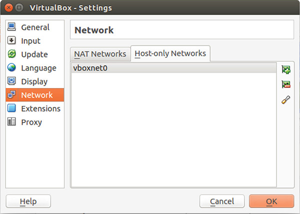
Figure 13-76 VirtualBox network settings.
K. Go to your guest VM setting and choose Network. Change the network settings to Host-Only Adapter, as shown in Figure 13-77. Click OK to close the wizard.
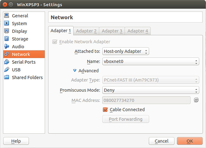
Figure 13-77 Guest VM network settings.
L. Check the IP address assigned to the virtual interface on the host machine by running ifconfig, as shown in Figure 13-78.
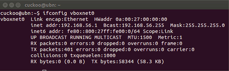
Figure 13-78 Check the IP address by running ifconfig.
M. Assign a static IP address to your guest VM so it belongs to the same subnet mask as the host, as shown in Figure 13-79.

Figure 13-79 TCP/IP properties.
N. You can test the connectivity between the host and the guest CM by making them ping each other, for example.
O. To give the guest VM Internet access through the host, you need to modify the iptables on the host. Assuming the host has a physical interface eth0 and a virtual interface vboxnet0 with subnet mask 192.168.56.0/24, add the following rules to your iptables:
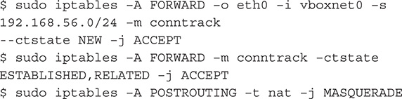
P. Finally, add IP forwarding.
![]()
Q. Your guest VM now has Internet access. Test it by browsing to a popular search page.
A. Copy the file cuckoo/agent/agent.py from the host to the guest VM. You can do so using the established shared folder.
![]()
B. Copy the agent.py file to the Startup folder on your guest VM. On a Windows XP machine, the location of the Startup folder is typically at C:Documents and Settings<user>Start MenuProgramsStartup. This will ensure that the agent is launched every time the guest VM is booted. When you execute the file, it spawns a Python window informing you that the agent started on the guest VM, as shown in Figure 13-80.

Figure 13-80 Cuckoo agent running in the guest VM.
C. Now is a good time to take a snapshot of the guest VM and to make a backup of the whole virtual machine.
5. Configure Cuckoo.
A. Before running Cuckoo, you need to configure some files on the host machine. All the configuration files are located under cuckoo/conf, and they are self-explanatory. You need to review the following files and make sure the settings match your environment:
![]() cuckoo.conf
cuckoo.conf
![]() auxillary.conf
auxillary.conf
![]() machinery.conf
machinery.conf
![]() reporting.conf
reporting.conf
B. For this installation, the configuration settings are as follows:
![]() Here is cuckoo.conf:
Here is cuckoo.conf:
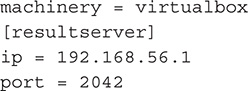
If you do not plan on using the default SQLite DBMS, you need to specify the connection string to your database in cuckoo.conf. For example, if you have MySQL installed on your host, your string will look like this:
![]()
where:
cuckooDB is the database name.
cuckoo is a user who has full privileges on cuckooDB.
{pass} is the password for the previous user.
![]() Here is auxillary.conf:
Here is auxillary.conf:

![]() Here is virtualbox.conf:
Here is virtualbox.conf:

WinXP is the name given to the guest VM, and 192.168.56.2 is its static IP address.
![]() Here is reporting.conf:
Here is reporting.conf:
![]()
This is important for the web interface to be able to pull data from the Mongo database.
C. As for the rest of the configuration files, there are no changes necessary.
6. Run Cuckoo.
A. Start Cuckoo by navigating to its directory on the host machine and running the following command:
![]()
B. You can submit a file for analysis using the following command line:
![]()
C. The submission Python script has many options. Please refer to the Cuckoo documentation to get more information on the usage of the submission tool.
D. For every file analyzed by the sandbox, Cuckoo assigns a task ID to it. Analysis reports are saved in cuckoo/storage/analysis. Use the task ID to find the corresponding subdirectory of the analysis files.
E. You can also submit samples using the web interface. First you will need to start the web server.
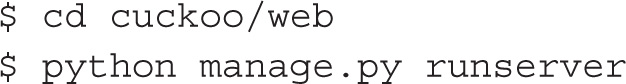
F. Now open a browser and navigate to http://localhost:8000/. The dashboard, as shown in Figure 13-81, gives you an overview of all the samples analyzed by the sandbox.

Figure 13-81 Cuckoo dashboard.
G. You can add more samples to the queue from the Submit page, as shown in Figure 13-82.

Figure 13-82 Cuckoo submit page.
H. To view the analysis report of a certain file on the web interface, you can use http://localhost:8000/analysis/<task_ID>/, where <task_ID> is the ID assigned by the analysis job upon file submission. Figure 13-83 shows an overview of an analyzed file.
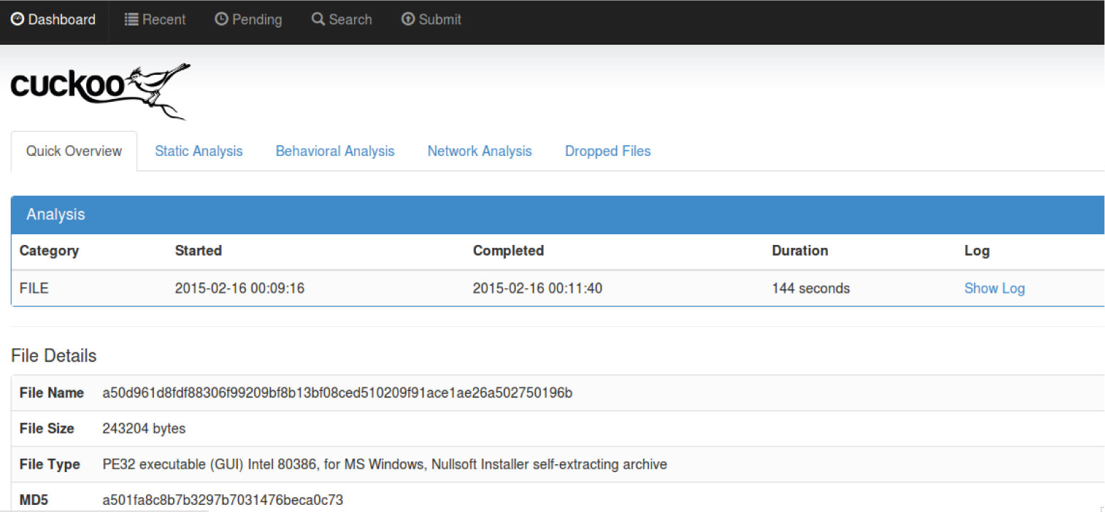
Figure 13-83 Cuckoo analysis overview.
7. Have fun playing with Cuckoo. You can also consult Cuckoo’s documentation for more features.
Free Online Automated Sandbox Services
Setting up your own sandbox requires a lot of effort, research, and trial and error, but once it is finished, the happiness and excitement you feel when you see your creation working is unmatched. But for those without the time and resources to set up their own sandbox, there are automated sandbox services that are offered online for free. Of course, there is a catch. Everything you submit may become property of these free services, so read carefully the terms of use and privacy policies of these services. Avoid sending files that may contain personally identifiable information (PII) or information that can be classified as intellectual property (IP). These services may also share this data with other third-party entities.
Free online automated sandbox services offer a quick and easy way to analyze a file. Some services will determine whether a file is malicious, while some will only give you a report, and it is up to you to deduce whether it is malicious.
The following are some of the more popular online automated sandbox services available for free:
![]() Anubis http://anubis.iseclab.org/
Anubis http://anubis.iseclab.org/
![]() Comodo Instant Malware Analysis http://camas.comodo.com/
Comodo Instant Malware Analysis http://camas.comodo.com/
![]() Comodo Valkyrie http://valkyrie.comodo.com/
Comodo Valkyrie http://valkyrie.comodo.com/
![]() EUREKA Malware Analysis Internet Service http://eureka.cyber-ta.org/
EUREKA Malware Analysis Internet Service http://eureka.cyber-ta.org/
![]() Malwr https://malwr.com/submission/
Malwr https://malwr.com/submission/
![]() MalwareViz https://www.malwareviz.com/
MalwareViz https://www.malwareviz.com/
![]() Payload Security https://www.hybrid-analysis.com/
Payload Security https://www.hybrid-analysis.com/
![]() ThreatExpert http://www.threatexpert.com/submit.aspx
ThreatExpert http://www.threatexpert.com/submit.aspx
![]() ThreatTrack Public Malware Sandbox http://www.threattracksecurity.com/resources/sandbox-malware-analysis.aspx
ThreatTrack Public Malware Sandbox http://www.threattracksecurity.com/resources/sandbox-malware-analysis.aspx
![]() VICheck https://www.vicheck.ca/
VICheck https://www.vicheck.ca/
NOTE
MalwareViz is used in tandem with Malwr. MalwareViz accepts malwr analysis link as its input.
Experiment on these different automated sandbox services and compare each of their outputs. You can see that some of them offer more information than others. Compare them also to the output of your Cuckoo sandbox. These free online automated services can be your benchmark when it comes to the effectiveness of your own sandbox implementation.
TIP
Do not limit yourself to one sandbox implementation. Always collect information about a malware from other sandboxes and combine them to paint an accurate picture of the malware.
Recap
In this chapter, I discussed the common malware analysis use cases and how they should determine what goes inside a malware analyst’s toolbox.
I also noted that regardless of the use case a malware analyst is trying to satisfy, there are tools that are considered indispensable when it comes to malware analysis. I call them tools of the trade. They are as follows:
![]() Sysinternals Suite
Sysinternals Suite
![]() Yara
Yara
![]() Cygwin
Cygwin
![]() Debuggers
Debuggers
![]() Disassemblers
Disassemblers
![]() Memory dumpers
Memory dumpers
![]() PE viewers
PE viewers
![]() PE reconstructors
PE reconstructors
![]() Malcode Analyst Pack
Malcode Analyst Pack
![]() Rootkit tools
Rootkit tools
![]() Network capturing tools
Network capturing tools
![]() Automated sandboxes
Automated sandboxes
![]() Free online automated sandbox services
Free online automated sandbox services
Combining these tools the right way gives analysts and researchers a potent weapon in tackling the most difficult malware. In this chapter, you combined these tools to solve the most challenging use cases analysts and researchers always face. They are as follows:
![]() Manually unpacking a packed malware
Manually unpacking a packed malware
![]() Analyzing a user mode rootkit
Analyzing a user mode rootkit
![]() Analyzing a kernel mode rootkit
Analyzing a kernel mode rootkit
It is important to note that there are more tools out there; the main thing is to find a tool that you are comfortable with and that satisfies your use cases.
Tools
![]() Sysinternals Suite https://technet.microsoft.com/en-us/sysinternals/bb842062.aspx
Sysinternals Suite https://technet.microsoft.com/en-us/sysinternals/bb842062.aspx
![]() Yara https://github.com/plusvic/yara
Yara https://github.com/plusvic/yara
![]() Cygwin https://www.cygwin.com
Cygwin https://www.cygwin.com
![]() Debuggers
Debuggers
![]() OllyDbg http://www.ollydbg.de/
OllyDbg http://www.ollydbg.de/
![]() Immunity Debugger http://debugger.immunityinc.com/
Immunity Debugger http://debugger.immunityinc.com/
![]() Windows debuggers
Windows debuggers
![]() WinDbg https://msdn.microsoft.com/en-us/windows/hardware/hh852365.aspx.
WinDbg https://msdn.microsoft.com/en-us/windows/hardware/hh852365.aspx.
![]() KD and NTKD https://msdn.microsoft.com/en-us/library/windows/hardware/hh406279%28v=vs.85%29.aspx
KD and NTKD https://msdn.microsoft.com/en-us/library/windows/hardware/hh406279%28v=vs.85%29.aspx
![]() Disassembler
Disassembler
![]() IDA https://www.hex-rays.com/products/ida/support/download.shtml
IDA https://www.hex-rays.com/products/ida/support/download.shtml
![]() Memory dumpers
Memory dumpers
![]() LordPE by y0da http://www.woodmann.com/collaborative/tools/index.php/LordPE
LordPE by y0da http://www.woodmann.com/collaborative/tools/index.php/LordPE
![]() Volatility Framework https://code.google.com/p/volatility/wiki/VolatilityIntroduction
Volatility Framework https://code.google.com/p/volatility/wiki/VolatilityIntroduction
![]() PE viewers
PE viewers
![]() Hiew http://www.hiew.ru/
Hiew http://www.hiew.ru/
![]() Heaventools PE Explorer http://www.heaventools.com/overview.htm
Heaventools PE Explorer http://www.heaventools.com/overview.htm
![]() PEview http://wjradburn.com/software/
PEview http://wjradburn.com/software/
![]() Dependency Walker http://www.dependencywalker.com/
Dependency Walker http://www.dependencywalker.com/
![]() Resource Hacker http://www.angusj.com/resourcehacker/
Resource Hacker http://www.angusj.com/resourcehacker/
![]() ImpREC by MackT http://www.woodmann.com/collaborative/tools/index.php/ImpREC
ImpREC by MackT http://www.woodmann.com/collaborative/tools/index.php/ImpREC
![]() Malcode Analyst Pack http://www.woodmann.com/collaborative/tools/index.php/Malcode_Analysis_Pack
Malcode Analyst Pack http://www.woodmann.com/collaborative/tools/index.php/Malcode_Analysis_Pack
![]() Rootkit tools
Rootkit tools
![]() Rootkit Unhooker http://www.antirootkit.com/software/RootKit-Unhooker.htm
Rootkit Unhooker http://www.antirootkit.com/software/RootKit-Unhooker.htm
![]() Rootkit Revealer http://download.cnet.com/RootkitRevealer/3000-2248_4-10543918.html
Rootkit Revealer http://download.cnet.com/RootkitRevealer/3000-2248_4-10543918.html
![]() Network capturing tools
Network capturing tools
![]() Wireshark https://www.wireshark.org/
Wireshark https://www.wireshark.org/
![]() TCPDump http://www.tcpdump.org/
TCPDump http://www.tcpdump.org/
![]() TCPView https://technet.microsoft.com/en-us/sysinternals/bb897437.aspx
TCPView https://technet.microsoft.com/en-us/sysinternals/bb897437.aspx
![]() OSR driver loader http://www.osronline.com/article.cfm?article=157
OSR driver loader http://www.osronline.com/article.cfm?article=157
![]() Automated sandboxes
Automated sandboxes
![]() Cuckoo http://www.cuckoosandbox.org/
Cuckoo http://www.cuckoosandbox.org/
![]() Free online automated sandbox services
Free online automated sandbox services
![]() Anubis http://anubis.iseclab.org/
Anubis http://anubis.iseclab.org/
![]() Comodo Instant Malware Analysis http://camas.comodo.com/
Comodo Instant Malware Analysis http://camas.comodo.com/
![]() Comodo Valkyrie http://valkyrie.comodo.com/
Comodo Valkyrie http://valkyrie.comodo.com/
![]() EUREKA Malware Analysis Internet Service http://eureka.cyber-ta.org/
EUREKA Malware Analysis Internet Service http://eureka.cyber-ta.org/
![]() Malwr https://malwr.com/submission/
Malwr https://malwr.com/submission/
![]() MalwareViz https://www.malwareviz.com/
MalwareViz https://www.malwareviz.com/
![]() Payload Security https://www.hybrid-analysis.com/
Payload Security https://www.hybrid-analysis.com/
![]() ThreatExpert http://www.threatexpert.com/submit.aspx
ThreatExpert http://www.threatexpert.com/submit.aspx
![]() ThreatTrack Public Malware Sandbox http://www.threattracksecurity.com/resources/sandbox-malware-analysis.aspx
ThreatTrack Public Malware Sandbox http://www.threattracksecurity.com/resources/sandbox-malware-analysis.aspx
![]() VICheck https://www.vicheck.ca/
VICheck https://www.vicheck.ca/
1 Yara: https://plusvic.github.io/yara/.
2 Cygwin: https://www.cygwin.com/.
3 Microsoft Technet: http://technet.microsoft.com/en-US/.
4 Cuckoo Sandbox: http://www.cuckoosandbox.org/.