
Chapter 5
Graphing Your Way to the Good Life
IN THIS CHAPTER
![]() Establishing the coordinate system
Establishing the coordinate system
![]() Using intercepts and symmetry to your advantage
Using intercepts and symmetry to your advantage
![]() Plotting lines on a graph
Plotting lines on a graph
![]() Reviewing the ten most common graphs in algebra
Reviewing the ten most common graphs in algebra
![]() Embracing technology with graphing calculators
Embracing technology with graphing calculators
An algebraic graph is a drawing that illustrates an algebraic relationship or equation in a two-dimensional plane (like a piece of graph paper). A graph allows you to see the characteristics of an algebraic statement immediately.
The graphs in algebra are unique because they reveal relationships that you can use to model situations. The graph of a mathematical curve has a ton of information crammed into an elegant package. (Okay, not everyone thinks that the graph of a parabola is elegant, but beauty is in the eye of the beholder.) For example, parabolas can model daily temperature, and a flat, S-shaped curve can model the number of people infected with the flu.
In this chapter, you find out how lines, parabolas, other polynomials, and radical curves all fit into the picture. I start off with a quick refresher on graphing basics. The rest of the chapter helps you become a more efficient grapher so you don’t have to plot a million points every time you need to create a graph. Along the way, I discuss using intercepts and symmetry and working with linear equations. I also provide you with a quick rundown of ten basic forms and equations you run into again and again in Algebra II. After you recognize a few landmarks, you can quickly sketch a reasonable graph of an equation. And to top it all off, you get some pointers on using a graphing calculator.
Coordinating Your Graphing Efforts
You do most graphing in algebra in the Cartesian coordinate system — a gridlike system where you plot points depending on the magnitude and signs of numbers. You may be familiar with the basics of graphing coordinates, (x, y) points, from Algebra I or junior-high math. Within the Cartesian coordinate system (which is named for the philosopher and mathematician Rene Descartes), you can plug-and-plot points to draw a curve, or you can take advantage of knowing a little something about what the graphs should look like. In either case, the coordinates and their respective plotted points fit together to give you a picture.
Identifying the parts of the coordinate plane
A coordinate plane (shown in Figure 5-1) features two intersecting axes — two perpendicular lines that cross at a point called the origin. The axes divide up the coordinate plane into four quadrants, usually numbered with Roman numerals starting in the upper right-hand corner and moving counterclockwise.

John Wiley & Sons, Inc.
FIGURE 5-1: Identifying all the players in the coordinate plane.
The horizontal line is called the x-axis, and the vertical line is called the y-axis. The scales on the axes are shown with little tick marks. Usually, you have the same scale on both axes — each tick mark may represent one unit or five units — but sometimes the plane needs to have two different scales. In any case, the scale on any one axis is the same all along that axis.
You identify points on the coordinate plane with numbers called coordinates, which come in ordered pairs — where the order matters. In the ordered pair (x, y), the first number is the x-coordinate; it tells you how far and in which direction the point is from the origin along the x-axis. The second number is the y-coordinate; it tells you how far from the origin and in which direction the point is along the y-axis. In Figure 5-1, you can see several points drawn in with their corresponding coordinates.
Plotting from dot to dot
Graphing in algebra isn’t quite as simple as a quick game of connect-the-dots, but the main concept is the same: You connect the points in the correct order, and you see the desired picture.
In the section “Looking at 10 Basic Forms,” later in this chapter, you discover the advantage of having at least a hint of what a graph is supposed to look like. But even when you have a pretty good idea of what you’re going to get, you still need the down-and-dirty ability to plot points.
For example, the list of points ![]()
![]() doesn’t mean too much, and the list doesn’t look all that informative when graphed. But if you connect the points in order, you get a picture. You can see the points and the corresponding picture in Figure 5-2.
doesn’t mean too much, and the list doesn’t look all that informative when graphed. But if you connect the points in order, you get a picture. You can see the points and the corresponding picture in Figure 5-2.

John Wiley & Sons, Inc.
FIGURE 5-2: Connecting the points in order creates a picture.
 In algebra, you usually have to create your set of points to graph. A problem gives you a formula or equation, and you determine the coordinates of the points that work in that equation. Your main goal is to sketch the graph after finding as few points as necessary. If you know what the general shape of the graph should be, all you need are a few anchor points to be on your way.
For instance, if you want to sketch the graph of ![]() , you can find some points (x, y) that make the equation true. Some points that work (picked at random, making sure they work in the equation) include:
, you can find some points (x, y) that make the equation true. Some points that work (picked at random, making sure they work in the equation) include: ![]()
![]() , and
, and ![]() . You can find many, many more points that work, but these points should give you a pretty good idea of what’s going on. In Figure 5-3a, you can see the points graphed; I connect them with a smooth curve in Figure 5-3b. The order of connecting the points goes by the order of the x-coordinates.
. You can find many, many more points that work, but these points should give you a pretty good idea of what’s going on. In Figure 5-3a, you can see the points graphed; I connect them with a smooth curve in Figure 5-3b. The order of connecting the points goes by the order of the x-coordinates.

John Wiley & Sons, Inc.
FIGURE 5-3: Creating a set of points to fit the graph of an equation.
Streamlining the Graphing Process with Intercepts and Symmetry
Graphing curves can take as long as you like or be as quick as you like. If you take advantage of the characteristics of the curves you’re graphing, you can cut down on the time it takes to graph and improve your accuracy. Two features that you can quickly recognize and solve for are the intercepts and symmetry of the graphs.
Finding x- and y-intercepts
The intercepts of a graph appear at the points where the lines of the graph cross the axes. The graph of a curve may never cross an axis, but when it does, knowing the points that represent the intercepts is very helpful.
The x-intercepts always have the format ![]() — the y-coordinate of an x-intercept is 0 because the point is on the x-axis. The y-intercepts have the form
— the y-coordinate of an x-intercept is 0 because the point is on the x-axis. The y-intercepts have the form ![]() — the x-coordinate is zero because the point is on the y-axis. You find the x- and y-intercepts by letting y and x, respectively, equal zero and solving for the other coordinate.
— the x-coordinate is zero because the point is on the y-axis. You find the x- and y-intercepts by letting y and x, respectively, equal zero and solving for the other coordinate.
For example, the graph of ![]() has two x-intercepts and one y-intercept:
has two x-intercepts and one y-intercept:
- To find the x-intercepts, let
 ; you then have the quadratic equation
  . You solve this equation by factoring it into
  . You find two solutions,
  and
and  , so the two x-intercepts are (3, 0) and
  . (For more on factoring, see Chapters 1 and 3.)
 - To find the y-intercept, let
 . This gives you the equation
  . The y-intercept, therefore, is (0, 6).
Figure 5-4a shows the intercepts of the previous example problem placed on the axes. The graph doesn’t tell you a whole lot unless you’re aware that the equation is a parabola. If you know that you have a parabola (which you will if you read Chapter 7), you know that a U-shaped curve goes through the intercepts. For now, you can just plug-and-plot to find a few more points to help you with the graph (see the section “Plotting from dot to dot”). Using the equation to find other points that work with the graph, you get ![]() , and
, and ![]() . Figure 5-4b shows the completed graph.
. Figure 5-4b shows the completed graph.

John Wiley & Sons, Inc.
FIGURE 5-4: Plotting the intercepts and calculated points on a graph to get the whole picture.
Reflecting on a graph’s symmetry
When an item or individual is symmetric, you can see a sameness or pattern to it. A graph that’s symmetric with respect to one of the axes appears to be a mirror image of itself on either side of the axis. A graph symmetric about the origin appears to be the same after a 180-degree turn. Figure 5-5 shows three curves and three symmetries: symmetry with respect to the y-axis (a), symmetry with respect to the x-axis (b), and symmetry with respect to the origin (c).

John Wiley & Sons, Inc.
FIGURE 5-5: Symmetry in a graph makes for a pretty picture.
Recognizing that the graph of a curve has symmetry helps you sketch the graph and determine its characteristics. The following sections outline ways to determine, from a graph’s equation, if symmetry exists.
With respect to the y-axis
Consider an equation in this form: ![]() in x’s. If replacing every x with –x doesn’t change the value of y, the curve is the mirror image of itself over the y-axis. The graph contains the points (x, y) and
in x’s. If replacing every x with –x doesn’t change the value of y, the curve is the mirror image of itself over the y-axis. The graph contains the points (x, y) and ![]() .
.
For example, the graph of the equation ![]() is symmetric with respect to the y-axis. If you replace each x with
is symmetric with respect to the y-axis. If you replace each x with ![]() , the equation remains unchanged. Replacing each x with
, the equation remains unchanged. Replacing each x with ![]() ,
, ![]() . The y-intercept is (0, 1). Some other points include
. The y-intercept is (0, 1). Some other points include ![]() and
and ![]() . Notice that the y is the same for both positive and negative x’s. With symmetry about the y-axis, for every point (x, y) on the graph, you also find
. Notice that the y is the same for both positive and negative x’s. With symmetry about the y-axis, for every point (x, y) on the graph, you also find ![]() . It’s easier to find points when an equation has symmetry because of the pairs. Figure 5-6 shows the graph of
. It’s easier to find points when an equation has symmetry because of the pairs. Figure 5-6 shows the graph of ![]() .
.

John Wiley & Sons, Inc.
FIGURE 5-6: A graph’s reflection over a vertical line.
With respect to the x-axis
Consider an equation in this form: ![]() in y’s. If replacing every y with
in y’s. If replacing every y with ![]() doesn’t change the value of x, the curve is the mirror image of itself over the x-axis. The graph contains the points (x, y) and
doesn’t change the value of x, the curve is the mirror image of itself over the x-axis. The graph contains the points (x, y) and ![]() .
.
For example, the graph of ![]() is symmetric with respect to the x-axis. When you replace each y with
is symmetric with respect to the x-axis. When you replace each y with ![]() , the x value remains unchanged. The x-intercept is (10, 0). Some other points on the graph include
, the x value remains unchanged. The x-intercept is (10, 0). Some other points on the graph include ![]() ; and
; and ![]() . Notice the pairs of points that have positive and negative values for y but the same value for x. This is where the symmetry comes in: The points have both positive and negative values — on both sides of the x-axis — for each x coordinate. Symmetry about the x-axis means that for every point (x, y) on the curve, you also find the point
. Notice the pairs of points that have positive and negative values for y but the same value for x. This is where the symmetry comes in: The points have both positive and negative values — on both sides of the x-axis — for each x coordinate. Symmetry about the x-axis means that for every point (x, y) on the curve, you also find the point ![]() . This symmetry makes it easy to find points and plot the graph. The graph of
. This symmetry makes it easy to find points and plot the graph. The graph of ![]() is shown in Figure 5-7.
is shown in Figure 5-7.

John Wiley & Sons, Inc.
FIGURE 5-7: A graph’s reflection over a horizontal line.
With respect to the origin
Consider an equation in this form: ![]() in x’s or
in x’s or ![]() in y’s. If replacing every variable with its opposite gives the same result as multiplying the entire equation by
in y’s. If replacing every variable with its opposite gives the same result as multiplying the entire equation by ![]() , the curve can rotate by 180 degrees about the origin and be its own image. The graph contains the points (x, y) and
, the curve can rotate by 180 degrees about the origin and be its own image. The graph contains the points (x, y) and ![]() .
.
For example, the graph of ![]() is symmetric with respect to the origin. When you replace every x and y with
is symmetric with respect to the origin. When you replace every x and y with ![]() and
and ![]() , you get
, you get ![]() , which is the same as multiplying everything through by
, which is the same as multiplying everything through by ![]() . The origin is both an x and a y-intercept. The other x-intercepts are (1, 0), (–1, 0), (3, 0), and
. The origin is both an x and a y-intercept. The other x-intercepts are (1, 0), (–1, 0), (3, 0), and ![]() . Other points on the graph of the curve include
. Other points on the graph of the curve include ![]() , and
, and ![]() . These points illustrate the fact that (x, y) and
. These points illustrate the fact that (x, y) and ![]() are both on the graph. Figure 5-8 shows the graph of
are both on the graph. Figure 5-8 shows the graph of ![]() (I changed the scale on the y-axis to make each tick-mark equal 10 units).
(I changed the scale on the y-axis to make each tick-mark equal 10 units).

John Wiley & Sons, Inc.
FIGURE 5-8: A graph revolving 180 degrees about the origin of the coordinate plane.
Graphing Lines
Lines are some of the simplest graphs to sketch. It takes only two points to determine the one and only line that exists in that place on the coordinate plane, so one simple method for graphing lines is to find two points — any two points — on the line. Another useful method is to use a point and the slope of the line. The method you choose is often just a matter of personal preference.
The slope of a line also plays a big role in comparing it with other lines that run parallel or perpendicular to it. The slopes of parallel and perpendicular lines are closely related to one another.
Finding the slope of a line
The slope of a line, m, has a complicated math definition, but it’s basically a number — positive or negative, large or small — that highlights some of the characteristics of the line, such as its steepness and direction. The numerical value of the slope tells you if the line slowly rises or drops from left to right or dramatically soars or falls from left to right. In order to find the slope and discover the properties of the line, you can use the equation of the line to solve for the information you need, or you can look at the graph of the line to get the general picture. If you opt to concentrate on the equation of the line, you can either look at a specific format of the line’s equation or you can solve for points on the line, which allows you to solve for the slope.
Identifying characteristics of a line’s slope
A line can have a positive or a negative slope. If a line’s slope is positive, the line rises from left to right. If the slope is negative, the line falls from left to right. The greater the absolute value (the value of the number without regard to the sign; in other words, the distance of the number from zero) of a line’s slope, the steeper the line is. For example, if the slope is a number between ![]() and 1, the line is rather flat. A slope of zero means that the line is absolutely horizontal.
and 1, the line is rather flat. A slope of zero means that the line is absolutely horizontal.
A vertical line doesn’t have a slope. This is tied to the fact that numbers go infinitely high, and math doesn’t have a highest number — you just say infinity. Only an infinitely high number can represent a vertical line’s slope, but usually, if you’re talking about a vertical line, you just say that the slope doesn’t exist.
Formulating the value of a line’s slope
You can determine the slope of a line, m, if you know two points on the line. The formula for finding the slope with this method involves finding the difference between the y-coordinates of the points and dividing that difference by the difference of the x-coordinates of the points.
 You find the slope of the line that goes through the points
 ![]() and
and ![]() with the formula
with the formula ![]() .
.
For example, to find the slope of the line that crosses the points ![]() and
and ![]() , you use the formula to get
, you use the formula to get ![]() . This line is fairly steep — the absolute value of
. This line is fairly steep — the absolute value of ![]() is 2 — and it falls as it moves from left to right, which makes it negative.
is 2 — and it falls as it moves from left to right, which makes it negative.
 When you use the slope formula, it doesn’t matter which point you choose to be
 ![]() — the order of the points doesn’t matter — but you can’t mix up the order of the two different coordinates. You can run a quick check by seeing if the coordinates of each point are above and below one another. Also, be sure that the y-coordinates are in the numerator; a common error is to have the difference of the y-coordinates in the denominator.
— the order of the points doesn’t matter — but you can’t mix up the order of the two different coordinates. You can run a quick check by seeing if the coordinates of each point are above and below one another. Also, be sure that the y-coordinates are in the numerator; a common error is to have the difference of the y-coordinates in the denominator.
Facing two types of equations for lines
Algebra II offers two different forms for the equation of a line. The first is the standard form, written ![]() , with the two variable terms on one side and the constant on the other side. The other form is the slope-intercept form, written
, with the two variable terms on one side and the constant on the other side. The other form is the slope-intercept form, written ![]() ; the y value is set equal to the product of the slope, m, and x, and the product is added to the y-coordinate of the y-intercept, b.
; the y value is set equal to the product of the slope, m, and x, and the product is added to the y-coordinate of the y-intercept, b.
Meeting high standards with the standard form
The standard form for the equation of a line is written ![]() . One example of such a line is
. One example of such a line is ![]() . You can find an infinite number of points that satisfy this equation; to name a few, you can use
. You can find an infinite number of points that satisfy this equation; to name a few, you can use ![]() , and
, and ![]() . It takes only two points to graph a line, so you can choose any two points and plot them on the coordinate plane to create your line.
. It takes only two points to graph a line, so you can choose any two points and plot them on the coordinate plane to create your line.
However, the standard form has more information than may be immediately apparent. You can determine, just by looking at the numbers in the equation, the intercepts and slope of the line. The intercepts, in particular, are great for graphing the line, and you can find them easily because they fall right on the axes.
The line ![]() has
has
- An x-intercept of

- A y-intercept of

- A slope of

To graph the line ![]() , you find the two intercepts,
, you find the two intercepts, ![]() and
and ![]() , plot them, and create the line. Figure 5-9 shows the two intercepts and the graph of the line. Note that the line falls as it moves from left to right, confirming the negative value of the slope from the formula
, plot them, and create the line. Figure 5-9 shows the two intercepts and the graph of the line. Note that the line falls as it moves from left to right, confirming the negative value of the slope from the formula ![]() .
.

John Wiley & Sons, Inc.
FIGURE 5-9: Graphing  , a line written in standard form, using its intercepts.
Picking off the slope-intercept form
When the equation of a line is written in the slope-intercept form, ![]() , you have good information right at your fingertips. The coefficient (a number multiplied with a variable or unknown quantity) of the x term, m, is the slope of the line. And the constant, b, is the y value of the y-intercept (the coefficient of the y term must be 1). With these two bits of information, you can quickly sketch the line.
, you have good information right at your fingertips. The coefficient (a number multiplied with a variable or unknown quantity) of the x term, m, is the slope of the line. And the constant, b, is the y value of the y-intercept (the coefficient of the y term must be 1). With these two bits of information, you can quickly sketch the line.
If you want to graph the line ![]() , for example, you first plot the y-intercept, (0, 5), and then count off the slope from that point. The slope of the line
, for example, you first plot the y-intercept, (0, 5), and then count off the slope from that point. The slope of the line ![]() is 2; think of the 2 as the slope fraction, with the y-coordinate on top and the x-coordinate on bottom. The slope then is
is 2; think of the 2 as the slope fraction, with the y-coordinate on top and the x-coordinate on bottom. The slope then is ![]() .
.
 Counting off the slope means to start at the y-intercept, move one unit to the right (for the 1 in the denominator of the previous fraction), and, from the point one unit to the right, count two units up (for the 2 in the numerator). This process gets you to another point on the line.
You connect the point you count off with the y-intercept to create your line. Figure 5-10 shows the intercept, an example of counting off, and the new point that appears one unit to the right and two units up from the intercept — the point (1, 7).

John Wiley & Sons, Inc.
FIGURE 5-10: A line with a slope of 2 is fairly steep.
Changing from one form to the other
You can graph lines by using the standard form or the slope-intercept form of the equations. If you prefer one form to the other — or if you need a particular form for an application you’re working on — you can change the equations to your preferred form by performing simple algebra:
- To change the equation
 to the slope-intercept form, you first subtract 2x from each side and then divide both sides by the
  multiplier on the y term:

In the slope-intercept form, you can quickly determine the slope and y-intercept,
 .
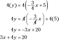
. - To change the equation
 to the standard form, you first multiply each side by 4 and then add 3x to each side of the equation:
Identifying parallel and perpendicular lines
Lines on the same coordinate plane are parallel if they never touch — no matter how far out you draw them. Lines are perpendicular when they intersect at a 90-degree angle. Both of these instances are fairly easy to spot when you see the lines graphed, but how can you be sure that the lines are truly parallel or that the angle is really 90 degrees and not 89.9 degrees? The answer lies in the slopes.
Consider two lines, ![]() and
and ![]() .
.
Two lines are parallel when their slopes are equal ![]() . Two lines are perpendicular when their slopes are negative reciprocals of one another
. Two lines are perpendicular when their slopes are negative reciprocals of one another ![]() .
.
For example, the lines ![]() and
and ![]() are parallel. Both lines have slopes of 3, but their y-intercepts are different — one crosses the y-axis at (0, 7) and the other at
are parallel. Both lines have slopes of 3, but their y-intercepts are different — one crosses the y-axis at (0, 7) and the other at ![]() . Figure 5-11a shows these two lines.
. Figure 5-11a shows these two lines.

John Wiley & Sons, Inc.
FIGURE 5-11: Parallel lines have equal slopes, and perpendicular lines have slopes that are negative reciprocals.
The lines ![]() and
and ![]() are perpendicular. The slopes are negative reciprocals of one another. You see these two lines graphed in Figure 5-11b.
are perpendicular. The slopes are negative reciprocals of one another. You see these two lines graphed in Figure 5-11b.
A quick way to determine if two numbers are negative reciprocals is to multiply them together; you should get a result of ![]() . For the previous example problem, you get
. For the previous example problem, you get ![]() .
.
Looking at 10 Basic Forms
You study many types of equations and graphs in Algebra II. You find very specific details on graphs of quadratics, other polynomials, radicals, rationals, exponentials, and logarithms in the various chapters of this book devoted to the different types. What I present in this section is a general overview of some of the types of graphs, designed to help you distinguish one type from another as you get ready to ferret out all the gory details. Knowing the basic graphs is the starting point for graphing variations on the basic graphs or more complicated curves.
Ten basic graphs seem to occur most often in Algebra II. I cover the first, a line, earlier in this chapter (see the section “Graphing Lines”), but I also include it in the following sections with the other nine basic graphs.
Lines and quadratics
Figure 5-12a shows the graph of a line. Lines can rise or drop as you move from left to right, or they can be horizontal or vertical. The line in Figure 5-12a has a positive slope and is fairly steep. For more details on lines and other figures, see the section “Graphing Lines.”
The slope-intercept equation of a line is ![]() .
.
Figure 5-12b shows a general quadratic (second-degree polynomial). This curve is called a parabola. Parabolas can open upward like this one, downward, to the left, or to the right. Figures 5-3, 5-4, and 5-5b earlier in the chapter show you some other quadratic curves. (Chapters 3 and 7 go into more quadratic detail.)
Two general equations for quadratics are ![]() and
and ![]() .
.

John Wiley & Sons, Inc.
FIGURE 5-12: Graphs of a steep line and an upward-facing quadratic.
Cubics and quartics
Figure 5-13a shows the graph of a cubic (third-degree polynomial). A cubic curve (a polynomial with degree 3) can be an S-shaped curve as shown, or it can flatten out in the middle and not feature those turns. A cubic can appear to come from below and end up high and to the right, or it can drop from the left, take some turns, and continue on down (for more on polynomials, check out Chapter 8).
The general equation for a cubic polynomial is ![]() .
.

John Wiley & Sons, Inc.
FIGURE 5-13: Graphs of an S-shaped cubic and a W-shaped quartic.
Figure 5-13b shows the graph of a quartic (fourth-degree polynomial). The graph has a distinctive W-shape, but that shape can flatten out, depending on how many terms appear in its equation. Similar to the quadratic (parabola), the quartic can open downward, in which case it looks like an M rather than a W.
The quartic polynomial has the following general equation: ![]()
![]() .
.
Radicals and rationals
In Figure 5-14a, you see a radical curve, and in Figure 5-14b, you see a rational curve. They seem like opposites, don’t they? But a major characteristic radical and rational curves have in common is that you can’t draw them everywhere. A radical curve can have an equation such as ![]() , where the square root doesn’t allow you to put values under the radical that give you a negative result. In this case, you can’t use any number smaller than four, so you have no graph when x is smaller than four. The radical curve in Figure 5-14a shows an abrupt stop at the left end, which is typical of a radical curve. (You can find more on radicals in Chapter 4.)
, where the square root doesn’t allow you to put values under the radical that give you a negative result. In this case, you can’t use any number smaller than four, so you have no graph when x is smaller than four. The radical curve in Figure 5-14a shows an abrupt stop at the left end, which is typical of a radical curve. (You can find more on radicals in Chapter 4.)

John Wiley & Sons, Inc.
FIGURE 5-14: Graphs of radicals often have abrupt stops, and graphs of rationals have gaps.
A general equation for some radical curves is ![]() , where n is a natural number.
, where n is a natural number.
Rational curves have a different type of restriction. When the equation of a curve involves a fraction, it opens itself up for the possibility of having a zero in the denominator of the fraction — a big no-no. You can’t have a zero in the denominator because math offers no such number, which is why the graphs of rational curves have spaces in them — places where the graph has a disconnect.
In Figure 5-14b, you see the graph of ![]() . The graph doesn’t have any value when
. The graph doesn’t have any value when ![]() . (Refer to Chapter 9 for information on rational functions.) A general equation for some rational curves is
. (Refer to Chapter 9 for information on rational functions.) A general equation for some rational curves is ![]() .
.
Exponential and logarithmic curves
Exponential and logarithmic curves are a type of opposites because the exponential and logarithmic functions are inverses of one another. Figure 5-15a shows you an exponential curve, and Figure 5-15b shows a logarithmic curve. When exponential curves are modeling physical situations (money, matter, temperature), they have a starting point, or initial value, of a, which is actually the y-intercept. The value of b determines whether the curve rises or falls in that gentle C shape. If b is larger than 1, the curve rises. If b is between 0 and 1, the curve falls. They generally rise or fall from left to right, but they face upward (called concave up). It helps to think of them collecting snow or sand in their gentle curves. Logarithmic curves also can rise or fall as you go from left to right, but they face downward.

John Wiley & Sons, Inc.
FIGURE 5-15: The graph of the exponential faces upward, and the graph of the logarithmic faces downward.
 Both exponential and logarithmic curves can model growth (or decay), where a previous amount is multiplied by some factor. The change continues on at the same rate throughout, so you produce steady curves up or down. (See Chapter 10 for more info on exponential and logarithmic functions.)
The general form for an exponential curve is ![]() .
.
The general form for a logarithmic curve is ![]() .
.
Absolute values and circles
The absolute value of a number is a positive value or 0, which is why you get a distinctive V-shaped curve from absolute value relations. Figure 5-16a shows a typical absolute value curve.
A general equation for an absolute value curve is ![]() .
.
The graph in Figure 5-16b is probably the most recognizable shape, except for the line, of the ten. A circle goes round and round a fixed distance from its center. (I cover circles and other conics in detail in Chapter 11.)
Circles with their centers at the origin have equations ![]() .
.

John Wiley & Sons, Inc.
FIGURE 5-16: Graphs of absolute values have distinctive V-shapes, and graphs of circles go round and round.
Solving Problems with a Graphing Calculator
You may think that discussions on graphing aren’t necessary if you have a calculator that does the graphing for you. Not so, Kemo Sabe. (If you aren’t a Lone Ranger fan, you can read the last sentence as, “Oh, that’s not true, you silly goose.”)
Graphing calculators are wonderful. They take much of the time-consuming drudgery out of graphing lines, curves, and all sorts of intricate functions. But you have to know how to use the calculator correctly and effectively. Two of the biggest stumbling blocks students and teachers face when using a graphing calculator to solve problems have to do with entering a function correctly and then finding the correct graphing window. You can use your calculator’s manual or online help to get all the other nitty-gritty details.
Entering equations into graphing calculators correctly
The trick to entering equations correctly into your graphing calculator is to insert what you mean (and mean what you insert). Your calculator will follow the order of operations, so you need to use parentheses to create the equation that you really want. (Refer to Chapter 1 if you need a review of the order of operations.) The four main trouble areas are fractions, exponents, radicals, and negative numbers.
Facing fractions
Say, for example, that you want to graph the equations ![]() ,
, ![]() , and
, and ![]() . You may mistakenly enter them into your graphing calculator as
. You may mistakenly enter them into your graphing calculator as ![]() ,
, ![]() , and
, and ![]() . They don’t appear at all as you expected. Why is that?
. They don’t appear at all as you expected. Why is that?
When you enter ![]() , your calculator (using order of operations) reads that as “Divide 1 by x and then add 2.” Instead of having a gap in the graph when
, your calculator (using order of operations) reads that as “Divide 1 by x and then add 2.” Instead of having a gap in the graph when ![]() , like you expect, the gap or discontinuity appears when
, like you expect, the gap or discontinuity appears when ![]() — your hint that you have a problem. If you want the numerator divided by the entire denominator, you use parentheses around the terms in the denominator. Enter the first equation as
— your hint that you have a problem. If you want the numerator divided by the entire denominator, you use parentheses around the terms in the denominator. Enter the first equation as ![]() .
.
Most graphing calculators try to connect the curves, even when you don’t want the curves to be connected. You see what appear to be vertical lines in the graph where you shouldn’t see anything (see the section “Disconnecting curves” later in this chapter).
If you enter the second equation as ![]() , the calculator does the division first, as dictated by the order of operations, and then adds x. You get the wrong rational curve, not the one you’re expecting. The correct way to enter this equation is
, the calculator does the division first, as dictated by the order of operations, and then adds x. You get the wrong rational curve, not the one you’re expecting. The correct way to enter this equation is ![]() .
.
The last equation, if entered as ![]() , may or may not come out correctly. Some calculators will grab the x and put it in the denominator of the fraction. Others will read the equation as
, may or may not come out correctly. Some calculators will grab the x and put it in the denominator of the fraction. Others will read the equation as ![]() times the x. To be sure, you should write the fraction in parentheses:
times the x. To be sure, you should write the fraction in parentheses: ![]() .
.
When you enter a division symbol, ![]() , in your calculator, the screen will show a slanted line, /. When you enter multiplication, your calculator will show an asterisk, *.
, in your calculator, the screen will show a slanted line, /. When you enter multiplication, your calculator will show an asterisk, *.
Figure 5-17 shows you how the three equations in this discussion will look in a typical graphing calculator.

John Wiley & Sons, Inc.
FIGURE 5-17: Equations entered in the y-menu of a graphing calculator.
Expressing exponents
Graphing calculators have some built-in exponents that make it easy to enter the expressions. You have a button for squared, 2, and, if you look hard, you can find one for cubed, 3. Calculators also provide an alternative to these options, and to all the other exponents: You can enter an exponent with a caret, ^ (pronounced carrot, like what Bugs Bunny eats).
You have to be careful when entering exponents with carets. When graphing ![]() or
or ![]() , you don’t get the correct graphs if you type
, you don’t get the correct graphs if you type ![]() and
and ![]() . Instead of getting a radical curve (raising to the
. Instead of getting a radical curve (raising to the ![]() power is the same as finding the square root) for
power is the same as finding the square root) for ![]() , you get a line. You need to put the fractional exponent in parentheses:
, you get a line. You need to put the fractional exponent in parentheses: ![]() . The same goes for the second curve. When you have more than one term in an exponent, you put the whole exponent in parentheses:
. The same goes for the second curve. When you have more than one term in an exponent, you put the whole exponent in parentheses: ![]() .
.
Raising Cain over radicals
Graphing calculators often have keys for square roots — and even other roots. The main problem comes if you don’t put every term that falls under the radical where it belongs.
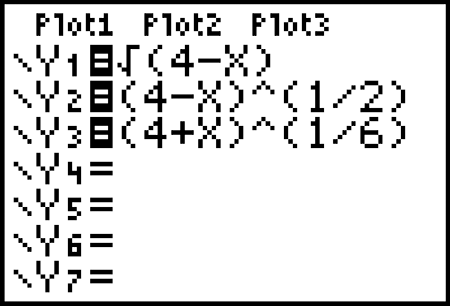
If you want to graph ![]() and
and ![]() , for example, you use parentheses around what falls under the radical and parentheses around any fractional exponents. Figure 5-18 shows two ways to enter the first and one way to enter the second the equation:
, for example, you use parentheses around what falls under the radical and parentheses around any fractional exponents. Figure 5-18 shows two ways to enter the first and one way to enter the second the equation:
John Wiley & Sons, Inc.
FIGURE 5-18: Radicals can be represented by fractional exponents.
Negating or subtracting
In all phases of algebra, you treat subtract, minus, opposite, and negative the same way, and they all have the same symbol, “![]() ”. Graphing calculators aren’t quite as forgiving. They have a special button for negative, and they have another button that means subtract.
”. Graphing calculators aren’t quite as forgiving. They have a special button for negative, and they have another button that means subtract.
If you’re performing the operation of subtraction, such as in ![]() , you use the subtract button found between the addition and multiplication buttons. If you want to type in the number
, you use the subtract button found between the addition and multiplication buttons. If you want to type in the number ![]() , you use the button with parentheses around the negative sign,
, you use the button with parentheses around the negative sign, ![]() . You get an error message if you enter the wrong one, but it helps to know why the action is considered an error.
. You get an error message if you enter the wrong one, but it helps to know why the action is considered an error.
Another problem with negatives has to do with the order of operations (see Chapter 1). If you want to square ![]() , you can’t enter
, you can’t enter ![]() into your calculator — if you do, you get the wrong answer. Your calculator squares the 4 and then takes its opposite, giving you
into your calculator — if you do, you get the wrong answer. Your calculator squares the 4 and then takes its opposite, giving you ![]() . To square the
. To square the ![]() , you put parentheses around both the negative sign and the
, you put parentheses around both the negative sign and the ![]() or
or ![]() .
.
Looking through the graphing window
Graphing calculators usually have a standard window to graph in — from ![]() to
to ![]() , both side-to-side and up-and-down. The standard window is a wonderful starting point and does the job for many graphs, but you need to know when to change the window or view of your calculator to solve problems.
, both side-to-side and up-and-down. The standard window is a wonderful starting point and does the job for many graphs, but you need to know when to change the window or view of your calculator to solve problems.
Using x-intercepts
The graph of ![]() appears only as a set of axes if you use the standard setting. The funky picture shows up because the two intercepts — (11, 0) and
appears only as a set of axes if you use the standard setting. The funky picture shows up because the two intercepts — (11, 0) and ![]() — don’t show up if you just go from
— don’t show up if you just go from ![]() to 10. (In Chapter 8, you find out how to determine these intercepts, if you’re not familiar with that process.) Knowing where the x-intercepts are helps you to set the window properly. You need to change the view or window on your calculator so that it includes all the intercepts. One possibility for the window of the example curve is to have the x-values go from
to 10. (In Chapter 8, you find out how to determine these intercepts, if you’re not familiar with that process.) Knowing where the x-intercepts are helps you to set the window properly. You need to change the view or window on your calculator so that it includes all the intercepts. One possibility for the window of the example curve is to have the x-values go from ![]() to 12 (one lower than the lowest and one higher than the highest).
to 12 (one lower than the lowest and one higher than the highest).
If you change the window in this fashion, you have to adjust the window upward and downward for the heights of the graph, or you can use Fit, a graphing capability of most graphing calculators. After you set how far to the left and right the window must go, you set the calculator to adjust the upward and downward directions with Fit. You have to tell the calculator how wide you want the graph to be. After you set the parameters, the Fit button automatically adjusts the height (up and down) so the window includes all the graph in that region.
Disconnecting curves
Your calculator, bless its heart, tries to be very helpful. But sometimes helpful isn’t accurate. For example, when you graph rational functions that have gaps, or graph piecewise functions that have holes, your calculator tries to connect the two pieces. You can just ignore the connecting pieces of graph, or you can change the mode of your calculator to dot mode. Most calculators have a Mode menu where you can change decimal values, angle measures, and so on. Go to that general area and toggle from connected to dot mode.
The downside to using dot mode is that sometimes you lose some of the curve — it won’t be nearly as complete as with the connected mode. As long as you recognize what’s happening with your calculator, you can adjust for its quirks.