Chapter 11
Cutting Up Conic Sections
IN THIS CHAPTER
![]() Grasping the layout of a sliced cone
Grasping the layout of a sliced cone
![]() Investigating the standard equations and graphs of the four conic sections
Investigating the standard equations and graphs of the four conic sections
![]() Properly identifying conics with nonstandard equations
Properly identifying conics with nonstandard equations
Conic is the name given to a special group of curves. What they have in common is how they’re constructed — points lying relative to an anchored point or points with respect to a line. But that sounds a bit stuffy, doesn’t it? Maybe it works better to think of conic sections in terms of how you can best describe the curves visually. Picture the Rainbow Bridge across the Niagara River. Imagine the earth’s path swinging around the sun. Reflect on the curved reflection plate in a car’s headlights. All these pictures circling your mind are related to curves called conics.
If you take a cone — imagine one of those yummy sugar cones that you put ice cream in — and slice it through in a particular fashion, the resulting edge you create will trace one of the four conic sections: a parabola, circle, ellipse, or hyperbola. (You can see a sketch of a cone in the following section. Hope it doesn’t make you too hungry!)
Each conic section has a specific equation, and I cover each thoroughly in this chapter. You can glean a good deal of valuable information from a conic section’s equation, such as where it’s centered in a graph, how wide it opens, and its general shape. I also discuss the techniques that work best for you when you’re called on to graph conics. Grab a pizza and an ice-cream cone for visual motivation and read on!
Cutting Up a Cone
A conic section is a curve formed by the intersection of a cone or two cones and a plane (a cone is a shape whose base is a circle and whose sides taper up to a point). The curve formed depends on where the cone is sliced:
- If you slice the cone straight across, you make the edge a circle, just like the top.
- If you slice a side piece off at an angle, you form a U-shaped parabola along the edge.
- If you slice the cone at a slant, you make the edge an ellipse, or an oval shape.
- If you picture two cones, tip to tip, and a slice going straight down through both, you picture a hyperbola. You have two wide, U-shaped edges that sort of come nose to nose. A hyperbola takes some special gymnastics!
Figure 11-1 shows each of the four conic sections sliced and diced. Each conic section has a specific equation that you use to graph the conic or to use it in an application (such as when the conic equation represents the curvature of a tunnel). You can head to the sections in this chapter that deal with the different conics to cover the topics in detail.

John Wiley & Sons, Inc.
FIGURE 11-1: The four conic sections.
Opening Every Which Way with Parabolas
A parabola, a U-shaped conic that I first introduce in Chapter 7 (the parabola is the only conic section that can fit the definition of a polynomial), is defined as all the points that fall the same distance from some fixed point, called its focus, and a fixed line, called its directrix. The focus is denoted by F, and the directrix by ![]() . Figure 11-2 shows you some of the points on a parabola and how they each appear the same distance from the parabola’s focus and directrix.
. Figure 11-2 shows you some of the points on a parabola and how they each appear the same distance from the parabola’s focus and directrix.

John Wiley & Sons, Inc.
FIGURE 11-2: Points on a parabola are the same distance away from a fixed point and line.
A parabola has a couple other defining features. The axis of symmetry of a parabola is a line that runs through the focus and is perpendicular to the directrix (imagine a line running through F in Figure 11-2). The axis of symmetry does just what its name suggests: It shows off how symmetric a parabola is. A parabola is a mirror image on either side of its axis. Another feature is the parabola’s vertex. The vertex is the curve’s extreme point — the lowest or highest point, or the point on the curve farthest right or farthest left. The vertex is also the point where the axis of symmetry crosses the curve (you can create this point by putting a pencil on the curve in Figure 11-2 where the imaginary axis crosses the curve after spearing through F).
Looking at parabolas with vertices at the origin
Parabolas can have graphs that go every which way and have vertices at any point in the coordinate system. When possible, though, you like to deal with parabolas that have their vertices at the origin. The equations are easier to deal with, and the applications are easier to solve. Therefore, I put the cart before the horse with this section to cover these specialized parabolas. (In the section “Observing the general form of parabola equations” later in the chapter, I deal with all the other parabolas you may run across.)
Opening to the right or left
Parabolas with their vertices (the plural form of vertex is vertices — just a little Latin for you) at the origin and opening to the right or left have a standard equation ![]() and are known as relations; you see a relationship between the variables. The standard form comes packed with information about the focus, directrix, vertex, axis of symmetry, and direction of a parabola. The equation also gives you a hint as to whether the parabola is narrow or opens wide.
and are known as relations; you see a relationship between the variables. The standard form comes packed with information about the focus, directrix, vertex, axis of symmetry, and direction of a parabola. The equation also gives you a hint as to whether the parabola is narrow or opens wide.
 The general form of a parabola with the equation
 ![]() gives you the following info:
gives you the following info:
- Focus: (a, 0)
- Directrix:

- Vertex: (0, 0)
- Axis of symmetry:

- Opening: To the right if a is positive; to the left if a is negative
- Shape: Narrow if
 is less than 1; wide if
  is greater than 1
 I use the absolute value operation,
 ![]() , instead of saying that 4a has to be between 0 and 1 or between
, instead of saying that 4a has to be between 0 and 1 or between ![]() and 0. I think it’s just a neater way of dealing with the rule.
and 0. I think it’s just a neater way of dealing with the rule.
For example, if you want to extract information about the parabola ![]() , you can put it in the
, you can put it in the ![]() form by writing it
form by writing it ![]() . In this case, you extract the following info:
. In this case, you extract the following info:
- The value of a is 2 (from
 ).
). - The focus is at (2, 0).
- The directrix is the line
 .
. - The vertex is at (0, 0).
- The axis of symmetry is
 .
. - The parabola opens to the right.
- The parabola is wide because
 is greater than 1.
Figure 11-3 shows the graph of the parabola ![]() with all the key information listed in the sketch.
with all the key information listed in the sketch.

John Wiley & Sons, Inc.
FIGURE 11-3: The parabola  with all its features on display.
Of course, extracting information is always more convenient when the equation of the parabola has an even-number coefficient, such as the 8 in ![]() , but the process works for odd numbers, too. You just have to deal with fractions. For instance, you can write the parabola
, but the process works for odd numbers, too. You just have to deal with fractions. For instance, you can write the parabola ![]() as
as ![]() , so the value of a is
, so the value of a is ![]() , the focus is
, the focus is ![]() , and so on. The value of a is just what it takes to multiply 4 by to get the coefficient.
, and so on. The value of a is just what it takes to multiply 4 by to get the coefficient.
Opening upward or downward
Parabolas that open left or right are relations, but parabolas that have curves opening upward or downward are a bit more special. The parabolas that open upward or downward are functions — they have only one y value for every x value. (For more on functions, refer to Chapter 6.) Parabolas of this variety with their vertex at the origin have the following standard equation: ![]() .
.
 You can tell that you have a relation (opening left or right) rather than a function (opening up or down) if the y variable is squared. The quadratic polynomials (from Chapter 7) and the functions all have the x variable squared.
The information you glean from the standard equation tells much the same story as the equation of parabolas that open sideways; however, many of the rules are reversed.
From the general form for the parabola ![]() , you extract the following information:
, you extract the following information:
- Focus: (0, a)
- Directrix:

- Vertex: (0, 0)
- Axis of symmetry:

- Opening: Upward if a is positive; downward if a is negative
- Shape: Narrow if
 is less than 1; wide if
  is greater than 1
You convert the parabola ![]() to the form
to the form ![]() because the general form gives you quick, easily accessible information. To perform the conversion, just divide the coefficient by 4, and then write the coefficient as 4 times the result of the division. You haven’t changed the value of the coefficient; you’ve just changed how it looks.
because the general form gives you quick, easily accessible information. To perform the conversion, just divide the coefficient by 4, and then write the coefficient as 4 times the result of the division. You haven’t changed the value of the coefficient; you’ve just changed how it looks.
In this case, you extract the following info:
- The value of a is
 .
. - The focus falls on the point
 .
. - The directrix forms a line at
 .
. - The vertex is at (0, 0).
- The axis of symmetry is
 .
. - The graph opens downward.
- The parabola is narrow because
 .
.
Figure 11-4 shows the graph of the parabola ![]() with all the elements illustrated in the sketch.
with all the elements illustrated in the sketch.

John Wiley & Sons, Inc.
FIGURE 11-4: A narrow parabola that opens downward.
Observing the general form of parabola equations
The curves of parabolas can open upward, downward, to the left, or to the right, but the curves don’t always have to have their vertices at the origin. Parabolas can wander all around a graph. So, how do you track the curves down to pin them on a graph? You look to their equations, which give you all the information you need to find out where they’ve wandered to.
When the vertex of a parabola is at the point (h, k), the general form for the equation is one of the following:
- Opening left or right:
 . When the y variable is squared, the parabola opens left or right. From this equation, just like with parabolas that have their vertices at the origin (see the previous section), you can extract information about the elements:
 - If 4a is positive, the curve opens right; if 4a is negative, the curve opens left.
- If
 , the parabola is relatively wide; if
  , the parabola is relatively narrow.
- Opening up or down:
 . When the x variable is squared, the parabola opens up or down. Here’s the info you can extract from this equation:
 - If 4a is positive, the parabola opens upward; if 4a is negative, the curve opens downward.
- If
 , the parabola is wide; if
  , the parabola is narrow.
The standard forms used for parabolas with their vertices at the origin (which I discuss in the previous sections) are special cases of these more general parabolas. If you replace the h and k coordinates with zeros, you have the special parabolas anchored at the origin.
A move in the position of the vertex (away from the origin, for example) changes the focus, directrix, and axis of symmetry of a parabola. In general, a move of the vertex just adds the value of h or k to the basic form. For instance, when the vertex is at (h, k), the focus is at ![]() for parabolas opening to the right and at
for parabolas opening to the right and at ![]() for parabolas opening upward. The directrix is also affected by h or k in its equation; it becomes
for parabolas opening upward. The directrix is also affected by h or k in its equation; it becomes ![]() for parabolas opening sideways and
for parabolas opening sideways and ![]() for those opening up or down. The whole graph shifts its position, but the shift doesn’t affect which direction it opens or how wide it opens. The shape and direction stay the same.
for those opening up or down. The whole graph shifts its position, but the shift doesn’t affect which direction it opens or how wide it opens. The shape and direction stay the same.
Sketching the graphs of parabolas
Parabolas have distinctive U-shaped graphs, and with just a little information, you can make a relatively accurate sketch of the graph of a particular parabola. The first step is to think of all parabolas as being in one of the general forms I list in the previous two sections. (Refer to the rules in the previous two sections when you graph a parabola.)
Taking the necessary graphing steps
Here’s the full list of steps to follow when sketching the graph of a parabola — either ![]() or
or ![]() :
:
 Determine the coordinates of the vertex, (h, k), and plot it.
If the equation contains
 or
or  , change the forms to
  or
or  , respectively, to determine the correct signs. Actually, you’re just reversing the sign that’s already there.
- Determine the direction the parabola opens, and decide if it’s wide or narrow, by looking at the 4a portion of the general parabola equation.
- Lightly sketch in the axis of symmetry that goes through the vertex (
 when the parabola opens upward or downward and
  when it opens sideways).
 - Choose a couple other points on the parabola and find each of their partners on the other side of the axis of symmetry to help you with the sketch.
For example, if you want to graph the parabola ![]() , you first note that this parabola has its vertex at the point
, you first note that this parabola has its vertex at the point ![]() and opens to the right, because the y is squared (if the x had been squared, it would open up or down) and a (2) is positive. The graph is relatively wide about the axis of symmetry,
and opens to the right, because the y is squared (if the x had been squared, it would open up or down) and a (2) is positive. The graph is relatively wide about the axis of symmetry, ![]() , because
, because ![]() , which makes
, which makes ![]() greater than 1. To find a random point on the parabola, try letting
greater than 1. To find a random point on the parabola, try letting ![]() and solve for
and solve for ![]() becomes
becomes ![]() . Square the 8 and then divide each side of the equation by 8 to get
. Square the 8 and then divide each side of the equation by 8 to get ![]() . Adding 1 to each side,
. Adding 1 to each side, ![]() ; so the point on the parabola is (9, 6).
; so the point on the parabola is (9, 6).
Another example point, which you find by using the same process that gave you (9, 6), is (5.5, 4). Figure 11-5 shows the vertex, axis of symmetry, and the two points placed in a sketch.

John Wiley & Sons, Inc.
FIGURE 11-5: A parabola sketched from points and lines deduced from the standard equation.
The two randomly chosen points have counterparts on the opposite side of the axis of symmetry. The point (9, 6) is 8 units above the axis of symmetry, so 8 units below the axis puts you at ![]() . The point (5.5, 4) is 6 units above the axis of symmetry, so its partner is the point
. The point (5.5, 4) is 6 units above the axis of symmetry, so its partner is the point ![]() .
.
Applying suspense to the parabola
Sketching parabolas helps you visualize how they’re used in an application, so you want to be able to sketch quickly and accurately if need be. A rather natural occurrence of a curve close to the parabola involves the cables that hang between the towers of a suspension bridge. These cables form a curve called a catenary, which is usually very close to a parabolic curve. Consider the following situation: An electrician wants to put a decorative light on the cable of a suspension bridge at a point 100 feet (horizontally) from where the cable touches the roadway at the middle of the bridge. You can see the electrician’s blueprint in Figure 11-6.

John Wiley & Sons, Inc.
FIGURE 11-6: The suspended cable on this bridge resembles a parabola.
The electrician needs to know how high the cable is at a point 100 feet from the center of the bridge so he can plan his lighting experiment. The towers holding the cable are 80 feet high, and the total length of the bridge is 400 feet.
You can help the electrician solve this problem by writing the equation of the parabola that fits all these parameters. The easiest way to handle the problem is to let the bridge roadbed be the x-axis and the center of the bridge be the origin (0, 0). The origin, therefore, is the vertex of the parabola. The parabola opens upward, so you use the equation of a parabola that opens upward with its vertex at the origin, which is ![]() (see the section “Looking at parabolas with vertices at the origin”).
(see the section “Looking at parabolas with vertices at the origin”).
To solve for a, you put the coordinates of the point (200, 80) in the equation. Where do you get these seemingly random numbers? Half the total of 400 feet of bridge is 200 feet. You move 200 feet to the right of the middle of the bridge and 80 feet up to get to the top of the right tower. Replacing the x in the equation with 200 and the y with 80, you get ![]() . Dividing each side of the equation by 80, you find that 4a is 500, so the equation of the parabola that represents the cable is
. Dividing each side of the equation by 80, you find that 4a is 500, so the equation of the parabola that represents the cable is ![]() .
.
So, how high is the cable at a point 100 feet from the center? In Figure 11-6, the point 100 feet from the center is to the left, so ![]() represents x. A parabola is symmetric about its vertex, so it doesn’t matter whether you use positive or negative 100 to solve this problem. But, sticking to the figure, let
represents x. A parabola is symmetric about its vertex, so it doesn’t matter whether you use positive or negative 100 to solve this problem. But, sticking to the figure, let ![]() in the equation; you get
in the equation; you get ![]() , which becomes
, which becomes ![]() . Dividing each side by 500, you get
. Dividing each side by 500, you get ![]() . The cable is 20 feet high at the point where the electrician wants to put the light. He needs a ladder!
. The cable is 20 feet high at the point where the electrician wants to put the light. He needs a ladder!
Converting parabolic equations to the standard form
When the equation of a parabola appears in standard form, you have all the information you need to graph it or to determine some of its characteristics, such as direction or size. Not all equations come packaged that way, though. You may have to do some work on the equation first to be able to identify anything about the parabola.
The standard form of a parabola is ![]() or
or ![]() , where (h, k) is the vertex.
, where (h, k) is the vertex.
The methods used here to rewrite the equation of a parabola into its standard form also apply when rewriting equations of circles, ellipses, and hyperbolas. (See the last section in this chapter, “Identifying Conics from Their Equations, Standard or Not,” for a more generalized view of changing the forms of conic equations.) The standard forms for conic sections are factored forms that allow you to immediately identify needed information. Different algebra situations call for different standard forms — the form just depends on what you need from the equation.
For instance, if you want to convert the equation ![]() into the standard form, you perform the following steps, which contain a method called completing the square (a method you use to solve quadratic equations; refer to Chapter 3 for a review of completing the square):
into the standard form, you perform the following steps, which contain a method called completing the square (a method you use to solve quadratic equations; refer to Chapter 3 for a review of completing the square):
- Rewrite the equation with the
 and x terms (or the
  and y terms) on one side of the equation and the rest of the terms on the other side.

Add a number to each side to make the side with the squared term into a perfect square trinomial (thus completing the square; see Chapter 3 for more on trinomials).
In this case, you add 25 to each side.
 simplifies to
  .
.- Rewrite the perfect square trinomial in factored form, and factor the terms on the other side by the coefficient of the variable.

You now have the equation in standard form. The vertex is at ![]() ; it opens upward and is fairly wide (see the section “Sketching the graphs of parabolas” to see how to make these determinations).
; it opens upward and is fairly wide (see the section “Sketching the graphs of parabolas” to see how to make these determinations).
Going Round and Round in Conic Circles
A circle, probably the most recognizable of the conic sections, is defined as all the points plotted at the same distance from a fixed point — the circle’s center, C. The fixed distance is the radius, r, of the circle.
The standard form for the equation of a circle with radius r and with its center at the point (h, k) is ![]() .
.
Figure 11-7 shows the sketch of a circle.

John Wiley & Sons, Inc.
FIGURE 11-7: All the points in a circle are the same distance from (h, k).
Standardizing the circle
When the equation of a circle appears in the standard form, it provides you with all you need to know about the circle: its center and radius. With these two bits of information, you can sketch the graph of the circle. The equation ![]() , for example, is the equation of a circle. You can change this equation to the standard form by completing the square for each of the variables (refer to Chapter 3 if you need a review of this process). Just follow these steps:
, for example, is the equation of a circle. You can change this equation to the standard form by completing the square for each of the variables (refer to Chapter 3 if you need a review of this process). Just follow these steps:
Change the order of the terms so that the x’s and y’s are grouped together and the constant appears on the other side of the equal sign.
Leave a space after the groupings for the numbers that you need to add:

Complete the square for each variable, adding the number that creates perfect square trinomials.
In the case of the x’s, you add 9, and with the y’s, you add 4. Don’t forget to also add 9 and 4 to the right:

When it’s simplified, you have
 .
.Factor each perfect square trinomial.
The standard form for the equation of this circle is
 .
.
The circle has its center at the point ![]() and has a radius of 4 (the square root of 16). To sketch this circle, you locate the point
and has a radius of 4 (the square root of 16). To sketch this circle, you locate the point ![]() and then count 4 units up, down, left, and right; sketch in a circle that includes those points. Figure 11-8 shows you the way.
and then count 4 units up, down, left, and right; sketch in a circle that includes those points. Figure 11-8 shows you the way.

John Wiley & Sons, Inc.
FIGURE 11-8: With the center, radius, and a compass, you too can sketch this circle.
Specializing in circles
Two circles you should consider special are: the circle with its center at the origin, and the unit circle.
A circle with its center at the origin has, of course, a center at (0, 0), so its standard equation becomes ![]() .
.
The equation of the center origin is simple and easy to work with, so you should take advantage of its simplicity and try to manipulate any application you’re working with that uses a circle into one with its center at the origin.
The unit circle also has its center at the origin, but it always has a radius of one. The equation of the unit circle is ![]() . This circle is also convenient and nice to work with. You use it to define trigonometric functions, and you find it in analytic geometry and calculus applications.
. This circle is also convenient and nice to work with. You use it to define trigonometric functions, and you find it in analytic geometry and calculus applications.
For example, a circle with its center at the origin and a radius of 5 units is created from the equation ![]() , where (h, k) is (0, 0) and
, where (h, k) is (0, 0) and ![]() ; therefore, it has the equation
; therefore, it has the equation ![]() . Any circle has an infinite number of points on it, but this clever choice for the radius gives you plenty of integers for coordinates. Points lying on the circle include
. Any circle has an infinite number of points on it, but this clever choice for the radius gives you plenty of integers for coordinates. Points lying on the circle include ![]()
![]() , and
, and ![]() . Not all circles offer this many integral coordinates, which is why this one is one of the favorites. (The rest of the infinite number of points on the circle have coordinates that involve fractions and radicals.)
. Not all circles offer this many integral coordinates, which is why this one is one of the favorites. (The rest of the infinite number of points on the circle have coordinates that involve fractions and radicals.)
Preparing Your Eyes for Solar Ellipses
The ellipse is considered the most aesthetically pleasing of all the conic sections. It has a nice oval shape often used for mirrors, windows, and art forms. Our solar system seems to agree: All the planets take an elliptical path around the sun.
The definition of an ellipse is all the points on a curve where the sum of the distances from any of those points to two fixed points is a constant. The two fixed points are the foci (plural of focus), denoted by F. Figure 11-9 illustrates this definition. You can pick a point on the ellipse, and the two distances from that point to the two foci sum to a number equal to any other distance sum from other points on the ellipse. In Figure 11-9, the distances from point A to the two foci are 3.2 and 6.8, which add to 10. The distances from point B to the two foci are 5 and 5, which also add to 10.

John Wiley & Sons, Inc.
FIGURE 11-9: The summed distances to the foci are equal for all points on an ellipse.
Raising the standards of an ellipse
You can think of the ellipse as a sort of squished circle. Of course, there’s much more to ellipses than that, but the label sticks because the standard equation of an ellipse has a vague resemblance to the equation for a circle (see the previous section).
The standard equation for an ellipse with its center at the point (h, k) is ![]() , where
, where
- x and y are points on the ellipse.
- a is half the length of the ellipse from left to right at its widest point.
- b is half the distance up or down the ellipse at its tallest point.
To be successful in elliptical problems, you need to find out more from the standard equation than just the center. You want to know if the ellipse is long and narrow or tall and slim. How long is it across, and how far up and down does it go? You may even want to know the coordinates of the foci. You can determine all these elements from the equation.
Determining the shape
An ellipse is criss-crossed by a major axis and a minor axis. Each axis divides the ellipse into two equal halves, with the major axis being the longer of the segments (such as the x-axis in Figure 11-9; if no axis is longer, you have a circle). The two axes intersect at the center of the ellipse. At the ends of the major axis, you find the vertices of the ellipse. Figure 11-10 shows two ellipses with their axes and vertices identified.

John Wiley & Sons, Inc.
FIGURE 11-10: Ellipses with their axis properties identified.
To determine the shape of an ellipse, you need to pinpoint two characteristics:
- Lengths of the axes: You can determine the lengths of the two axes from the standard equation of the ellipse. You take the square roots of the numbers in the denominators of the fractions. Whichever value is larger, a or b, tells you which is the major axis. The square roots of the numbers in the denominator represent the distances from the center to the points on the ellipse at the end of their respective axes. In other words, a is half the length of one axis, and b is half the length of the other. Therefore, 2a and 2b are the lengths of the axes.
To find the lengths of the major and minor axes of the ellipse
 , for example, you take the square roots of 25 and 49. The square root of the larger number, the 49, is 7. Twice 7 is 14, so the major axis is 14 units long. The square root of 25 is 5, and twice 5 is 10. The minor axis is 10 units long.
 - Assignment of the axes: The positioning of the axes is significant. The denominator that falls under the x signifies the axis that runs parallel to the x-axis. In the previous example, the 25 falls under the x, so the minor axis runs horizontal. The denominator that falls under the y factor is the axis that runs parallel to the y-axis. In the previous example, 49 falls under the y, so the major axis runs up and down parallel to the y-axis. This is a tall, narrow ellipse.
Finding the foci
You can find the two foci of an ellipse by using information from the standard equation. The foci, for starters, always lie on the major axis. They lie c units from the center. To find the value of c, you use parts of the ellipse equation to form the equation ![]() or
or ![]() , depending on which is larger,
, depending on which is larger, ![]() or
or ![]() . The value of
. The value of ![]() has to be positive.
has to be positive.
In the ellipse ![]() , for example, the major axis runs across the ellipse, parallel to the x-axis (see the previous section to find out why). Actually, the major axis is on the x-axis, because the center of this ellipse is the origin. You know this because the h and k are missing from the equation (actually, they’re both equal to zero). You find the foci of this ellipse by solving the foci equation:
, for example, the major axis runs across the ellipse, parallel to the x-axis (see the previous section to find out why). Actually, the major axis is on the x-axis, because the center of this ellipse is the origin. You know this because the h and k are missing from the equation (actually, they’re both equal to zero). You find the foci of this ellipse by solving the foci equation: ![]() . Substituting 25 for
. Substituting 25 for ![]() and 9 for
and 9 for ![]() , you have
, you have ![]() . Taking the square root,
. Taking the square root, ![]() .
.
So, the foci are 4 units on either side of the center of the ellipse. In this case, the coordinates of the foci are ![]() and (4, 0). Figure 11-11 shows the graph of the ellipse with the foci identified.
and (4, 0). Figure 11-11 shows the graph of the ellipse with the foci identified.

John Wiley & Sons, Inc.
FIGURE 11-11: The foci always lie on the major axis (in this case on the x-axis).
Also, for this example ellipse, the major axis is 10 units long, running from ![]() to (5, 0). These two points are the vertices. The minor axis is 6 units long, running from (0, 3) down to
to (5, 0). These two points are the vertices. The minor axis is 6 units long, running from (0, 3) down to ![]() .
.
When the center of the ellipse isn’t at the origin, you find the foci the same way and adjust for the center. The ellipse ![]() has its center at
has its center at ![]() . You find the foci by solving
. You find the foci by solving ![]() , which, in this case, is
, which, in this case, is ![]() . The value of c is either 24 (the root of 576) or
. The value of c is either 24 (the root of 576) or ![]() from the center, so the foci are (23, 3) and
from the center, so the foci are (23, 3) and ![]() . The major axis is
. The major axis is ![]() units, and the minor axis is
units, and the minor axis is ![]() units. The 25 and 7 come from the square roots of 625 and 49, respectively. And the vertices, the endpoints of the major axis, are at (24, 3) and
units. The 25 and 7 come from the square roots of 625 and 49, respectively. And the vertices, the endpoints of the major axis, are at (24, 3) and ![]() .
.
Sketching an elliptical path
Have you ever been in a whispering gallery? I’m talking about a room or auditorium where you can stand at a spot and whisper a message, and a person standing a great distance away from you can hear your message. This phenomenon was much more impressive before the days of hidden microphones, which tend to make us more skeptical of how this works. Anyway, here’s the algebraic principle behind a whispering gallery. You’re standing at one focus of an ellipse, and the other person is standing at the other focus. The sound waves from one focus reflect off the surface or ceiling of the gallery and move over to the other focus.
Suppose you run across a problem on a test that asks you to sketch the ellipse associated with a whispering gallery that has foci 240 feet apart and a major axis (length of the room) of 260 feet. Your first task is to construct the equation of the ellipse.
The foci are 240 feet apart, so they each stand 120 feet from the center of the ellipse. The major axis is 260 feet long, so the vertices are each 130 feet from the center. Using the equation ![]() — which gives the relationship between c, the distance of a focus from the center; a, the distance from the center to the end of the major axis; and b, the distance from the center to the end of the minor axis — you get
— which gives the relationship between c, the distance of a focus from the center; a, the distance from the center to the end of the major axis; and b, the distance from the center to the end of the minor axis — you get ![]() . Armed with the values of
. Armed with the values of ![]() and
and ![]() , you can write the equation of the ellipse representing the curvature of the ceiling:
, you can write the equation of the ellipse representing the curvature of the ceiling: ![]() .
.
To sketch the graph of this ellipse, you first locate the center at (0, 0). You count 130 units to the right and left of the center and mark the vertices, and then you count 50 units up and down from the center for the endpoints of the minor axis. You can sketch the ellipse by using these endpoints. The sketch in Figure 11-12 shows the points described and the ellipse. It also shows the foci — where the two people would stand in the whispering gallery.

John Wiley & Sons, Inc.
FIGURE 11-12: A whispering gallery is long and narrow.
Feeling Hyper about Hyperbolas
The hyperbola is a conic section that seems to be in combat with itself. It features two completely disjoint curves, or branches, that face away from one another but are mirror images across a line that runs halfway between them.
A hyperbola is defined as all the points such that the difference of the distances between two fixed points (called foci) is a constant value. In other words, you pick a value, such as the number 6; you find two distances whose difference is 6, such as 10 and 4; and then you find a point that rests 10 units from the one point and 4 units from the other point. The hyperbola has two axes, just as the ellipse has two axes (see the previous section). The axis of the hyperbola that goes through its two foci is called the transverse axis. The other axis, the conjugate axis, is perpendicular to the transverse axis, goes through the center of the hyperbola, and acts as the mirror line for the two branches. Figure 11-13 shows two hyperbolas with their axes and foci identified. Figure 11-13a shows the distances P and q. The difference between these two distances to the foci is a constant number (which is true no matter what points you pick on the hyperbola).

John Wiley & Sons, Inc.
FIGURE 11-13: The curves of hyperbolas face away from one another.
There are two basic equations for hyperbolas. You use one when the hyperbola opens to the left and right: ![]() . You use the other when the hyperbola opens upward and downward:
. You use the other when the hyperbola opens upward and downward: ![]() . In both cases, the center of the hyperbola is at (h, k), and the foci are c units away from the center, where the relationship
. In both cases, the center of the hyperbola is at (h, k), and the foci are c units away from the center, where the relationship ![]() describes the relationship between the different parts of the equation. For example,
describes the relationship between the different parts of the equation. For example, ![]() is the equation of a hyperbola with its center at
is the equation of a hyperbola with its center at ![]() , which opens left and right; its foci are 5 units left and right of the center, so they’re at
, which opens left and right; its foci are 5 units left and right of the center, so they’re at ![]() and
and ![]() . You solve for c by using
. You solve for c by using ![]() , which, in this case, is
, which, in this case, is ![]() , giving you
, giving you ![]() or
or ![]() .
.
Including the asymptotes
A very helpful tool you can use to sketch hyperbolas is to first lightly sketch in the two diagonal asymptotes of the hyperbola. Asymptotes aren’t actual parts of the graph; they just help you determine the shape and direction of the curves. The asymptotes of a hyperbola intersect at the center of the hyperbola. You find the equations of the asymptotes by replacing the 1 in the equation of the hyperbola with a zero and simplifying the resulting equation into the equations of two lines.
If you want to find the equations of the asymptotes of the hyperbola ![]() , for example, you change the one to zero and then set the two fractions equal to one another:
, for example, you change the one to zero and then set the two fractions equal to one another:
is then written
.
Take the square root of each side:
simplifies to
.
Now you multiply each side by 4 to get the equations of the asymptotes in better form:
becomes
.
Consider the two cases — one using the positive sign, and the other using the negative sign. When using the positive sign, ![]() giving you
giving you ![]() or
or ![]() .
.
And, with the negative sign, ![]() becomes
becomes ![]() . Adding 4 to each side, you get
. Adding 4 to each side, you get ![]() or
or ![]() .
.
The two asymptotes you find are ![]() and
and ![]() , and you can see them in Figure 11-14. Notice that the slopes of the lines are the opposites of one another. (For a refresher on graphing lines, see Chapter 2.)
, and you can see them in Figure 11-14. Notice that the slopes of the lines are the opposites of one another. (For a refresher on graphing lines, see Chapter 2.)

John Wiley & Sons, Inc.
FIGURE 11-14: The asymptotes help you sketch the hyperbola.
Graphing hyperbolas
Hyperbolas are relatively easy to sketch, if you pick up the necessary information from the equations (see the intro to this section). To graph a hyperbola, use the following steps as guidelines:
Determine if the hyperbola opens to the sides or up and down by noting whether the x term is first or second.
The x term first means it opens to the sides.
- Find the center of the hyperbola by looking at the values of h and k.
Lightly sketch in a rectangle twice as wide as the square root of the denominator under the x value and twice as high as the square root of the denominator under the y value.
The rectangle’s center is the center of the hyperbola.
- Lightly sketch in the asymptotes through the vertices of the rectangle (see the previous section to find out how).
- Draw in the hyperbola, making sure it touches the midpoints of the sides of the rectangle.
You can use these steps to graph the hyperbola ![]() . First, note that this equation opens to the left and right because the x value comes first in the equation. The center of the hyperbola is at
. First, note that this equation opens to the left and right because the x value comes first in the equation. The center of the hyperbola is at ![]() .
.
Now comes the mysterious rectangle. In Figure 11-15a, you see the center placed on the graph at ![]() . You count 3 units to the right and left of center (totaling 6), because twice the square root of 9 is 6. Now you count 4 units up and down from center, because twice the square root of 16 is 8. A rectangle 6 units wide and 8 units high is shown in Figure 11-15b.
. You count 3 units to the right and left of center (totaling 6), because twice the square root of 9 is 6. Now you count 4 units up and down from center, because twice the square root of 16 is 8. A rectangle 6 units wide and 8 units high is shown in Figure 11-15b.

John Wiley & Sons, Inc.
FIGURE 11-15: Drawing a rectangle before drawing the hyperbola is a sketching help.
When the rectangle is in place, you draw in the asymptotes of the hyperbola diagonally through the vertices (corners) of the rectangle. Figure 11-16a shows the asymptotes drawn in. The equations of those asymptotes are ![]() and
and ![]() (see the previous section to calculate these equations). Note: When you’re just sketching the hyperbola, you usually don’t need the equations of the asymptotes.
(see the previous section to calculate these equations). Note: When you’re just sketching the hyperbola, you usually don’t need the equations of the asymptotes.

John Wiley & Sons, Inc.
FIGURE 11-16: The hyperbola takes its shape with the asymptotes in place.
Lastly, with the asymptotes in place, you draw in the hyperbola, making sure it touches the sides of the rectangle at its midpoints and slowly gets closer and closer to the asymptotes as the curves get farther from the center. You can see the full hyperbola in Figure 11-16b.
Identifying Conics from Their Equations, Standard or Not
When you write the equations of the four conic sections in their standard forms, you can easily tell which type of conic you have most of the time.
- A parabola has only one squared variable:

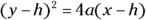 or
or 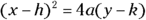
- A circle can be written without the variables in fractions:

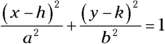
- An ellipse shows a sum of the two variable terms (at least one as a fraction):
- A hyperbola shows a difference of the two variable terms:
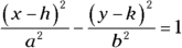 or
or 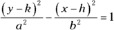
Sometimes, however, the equation you’re given isn’t in standard form. It has yet to be changed, using completing the square (see Chapter 3) or whatever method it takes. So, in these situations, how do you tell which type of conic you have by just looking at the equation (without having to rewrite the form)?
Consider all the equations of the form ![]() . You have squared terms and first-degree terms of the two variables x and y. By observing what A, B, C, and D are, you can determine which type of conic you have.
. You have squared terms and first-degree terms of the two variables x and y. By observing what A, B, C, and D are, you can determine which type of conic you have.
When you have an equation in the form ![]() , follow these rules:
, follow these rules:
- If
 , you have a circle (as long as A and B don’t equal zero).
 - If
 , and A and B are the same sign, you have an ellipse.
 - If A and B are different signs, you have a hyperbola.
- If A or B is zero, you have a parabola (they can’t both be zero).
Use these rules to determine which conic you have from some equations:
 is an ellipse, because
  , and A and B are both positive. In fact, the standard form for this equation (which you find by completing the square) is
 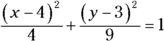 .
. is a circle, because
  . Its standard form is
  .
. is a hyperbola, because A and B have opposite signs. This hyperbola’s standard form is
 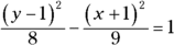 .
. is a parabola. You see only an
  term — the only variable raised to the second power. The standard form for this parabola is
 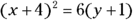 .
.