Sizing up domain

As I explain in Chapter 6, the domain of a function consists of all the real numbers that you can use in the function equation. Values in the domain have to work in the equation and avoid producing imaginary or nonexistent answers.

You write the equations of rational functions as fractions — and fractions have denominators. The denominator of a fraction can’t equal zero, so you exclude anything that makes the denominator of a rational function equal to zero from the domain of the function.

The following list illustrates examples of domains of selected rational functions:

• The domain of is all real numbers except 2. In interval notation (see Chapter 2), you write the domain as . (The symbol signifies that the numbers increase without end; and the signifies decreasing without end. The between the two parts of the answer means or.)
• The domain of is all real numbers except 0 and . In interval notation, you write the domain as .
• The domain of is all real numbers; no number makes the denominator equal to zero. You can write the domain as .

Introducing intercepts

Functions in algebra can have intercepts. A rational function may have some x - intercepts and/or a y - intercept, but it doesn’t have to have either. You can determine whether a given rational function has intercepts by looking at its equation.

Determining the equations of vertical asymptotes

The equations of vertical asymptotes appear in the form . This equation of a line has only the x variable — no y variable — and the number h. A vertical asymptote occurs in the rational function if f(x) and g(x) have no common factors, and it appears at whatever values the denominator equals zero — . (In other words, vertical asymptotes occur at values that don’t fall in the domain of the rational function.)

A discontinuity is a place where a rational function doesn’t exist — you find a break in the flow of the numbers being used in the function equation (the domain). A discontinuity is indicated by a numerical value that tells you where the function isn’t defined; this number isn’t in the domain of the function. You know that a function is discontinuous wherever a vertical asymptote appears in the graph because vertical asymptotes indicate breaks or gaps in the domain.

To find the vertical asymptotes of the function , for example, you first note that there’s no common factor in the numerator and denominator. Then you set the denominator equal to zero. Factoring , you get . The solutions are and , which are the equations of the vertical asymptotes.

Determining the equations of horizontal asymptotes

The horizontal asymptote of a rational function has an equation that appears in the form . This linear equation has only the variable y — no x — and the k is some number. A rational function has only one horizontal asymptote — if it has one at all (some rational functions have no horizontal asymptotes, others have one, and none of them have more than one). A rational function has a horizontal asymptote when the degree (highest power) of f(x), the polynomial in the numerator, is less than or equal to the degree of g(x), the polynomial in the denominator.

Here’s a rule for determining the equation of a horizontal asymptote. The horizontal asymptote of is when , meaning that the highest degrees of the polynomials in the numerator and denominator are the same. The fraction here is made up of the lead coefficients of the two polynomials. When , meaning that the degree in the numerator is less than the degree in the denominator, then the horizontal asymptote is .

If you want to find the horizontal asymptote of , for example, you use the previously stated rules. Because , the horizontal asymptote is . Now look at what happens when the degree of the denominator is the same as the degree of the numerator. The horizontal asymptote of is ( over ). The fraction formed by the lead coefficients is .

Graphing vertical and horizontal asymptotes

When a rational function has one vertical asymptote and one horizontal asymptote, its graph usually looks like two flattened-out, C-shaped curves that appear diagonally opposite one another from the intersection of the asymptotes. Occasionally, the curves appear side by side, but that’s the exception rather than the rule. Figure 9-1 shows you two examples of the more frequently found graphs in the one horizontal and one vertical classification. Note: The asymptotes are graphed with dashes rather than solid lines to emphasize that they are not really a part of the graph of the function.

In both graphs, the vertical asymptotes are at , and the horizontal asymptotes are at . In Figure 9-1a, the intercepts are and (2, 0). Figure 9-1b has intercepts of and (0, 1).

You can have only one horizontal asymptote in a rational function, but you can have more than one vertical asymptote. Typically, the curve to the right of the right-most vertical asymptote and to the left of the left-most vertical asymptote are like flattened-out or slowly turning C’s. They nestle in the corner and follow along the asymptotes. Between the vertical asymptotes is where some graphs get more interesting. Some graphs between vertical asymptotes can be U-shaped, going upward or downward (see Figure 9-2a), or they can cross in the middle, clinging to the vertical asymptotes on one side or the other (see Figure 9-2b). You find out which case you have by calculating a few points — intercepts and a couple more — to give you clues as to the shape. The graphs in Figure 9-2 show you some of the possibilities.

In Figure 9-2, the vertical asymptotes are at and . The horizontal asymptotes are at . Figure 9-2a has two x-intercepts lying between the two vertical asymptotes; the y-intercept is there, too. In Figure 9-2b, the y-intercept and one x-intercept lie between the two vertical asymptotes; another x-intercept is to the right of the right-most vertical asymptote.

The graph of a rational function can cross a horizontal asymptote, but it never crosses a vertical asymptote. Horizontal asymptotes show what happens for very large or very small values of x.

Crunching the numbers and graphing oblique asymptotes

An oblique or slant asymptote takes the form . You may recognize this form as the slope-intercept form for the equation of a line (as seen in Chapter 5). A rational function has a slant asymptote when the degree of the polynomial in the numerator is exactly one value greater than the degree in the denominator ( over , for example).

You can find the equation of the slant asymptote by using long division. You divide the denominator of the rational function into the numerator and use the first two terms in the answer. Those two terms are the part of the equation of the slant asymptote.

To find the slant asymptote of , for example, do the long division:

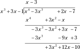
You can ignore the remainder at the bottom. The slant asymptote for this example is . (For more on long division of polynomials, see Algebra I Workbook For Dummies, written by yours truly and published by Wiley.)

An oblique (or slant) asymptote creates two new possibilities for the graph of a rational function. If a function has an oblique asymptote, its curve tends to be a very-flat C on opposite sides of the intersection of the slant asymptote and a vertical asymptote (see Figure 9-3a), or the curve has U-shapes between the asymptotes (see Figure 9-3b).

Figure 9-3a has a vertical asymptote at and a slant asymptote at ; its intercepts are at (0, 0) and (2, 0). Figure 9-3b has a vertical asymptote at and a slant asymptote at ; its only intercept is at (0, 0).

Removal by factoring

Discontinuities are removed when they no longer have an effect on the rational function equation. You know this is the case when you find a factor that’s common to both the numerator and the denominator. You accomplish the removal process by factoring the polynomials in the numerator and denominator of the rational function and then reducing the fraction.

To remove the discontinuity in the rational function , for example, you first factor the numerator and denominator of the fraction (see Chapter 3): .

Now you reduce the fraction to the new function statement: 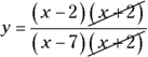giving you .

By getting rid of the removable discontinuity, you simplify the equation that you’re graphing. It’s easier to graph a line with a little hole in it than deal with an equation that has a fraction — and all the computations involved.

Evaluating the removal restrictions

The function, which you work with in the previous section, starts out with a quadratic in the denominator (see Chapters 3 and 7). You factor the denominator, and when you set it equal to zero, you find that the solutions and don’t appear in the domain of the function. Now what?

Numbers excluded from the domain stay excluded even after you remove the discontinuity. The function still isn’t defined for the two values you find. Therefore, you can conclude that the function behaves differently at each of the discontinuities. When , the graph of the function has a hole; the curve approaches the value, skips it, and goes on. It behaves in a reasonable fashion: The function values skip over the discontinuity, but the values get really close to it. When , however, a vertical asymptote appears; the discontinuity doesn’t go away. The function values go haywire at that x value and don’t settle down at all.

Showing removable discontinuities on a graph

A vertical asymptote of a rational function indicates a discontinuity, or a place on its graph where the function isn’t defined. On either side of a vertical asymptote, the graph rises toward positive infinity or falls toward negative infinity. The rational function has no limit wherever you see a vertical asymptote (see the “Pushing the Limits of Rational Functions” section later in the chapter). Some rational functions may have discontinuities at which limits exist. When a function has a removable discontinuity, a limit exists, and its graph shows this by putting a hollow circle in place of a piece of the graph.

Figure 9-4 shows a rational function with a vertical asymptote at and a removable discontinuity at . The horizontal asymptote is the x-axis (written ). Unfortunately, graphing calculators don’t show the little hollow circles indicating removable discontinuities. Oh, sure, they leave a gap there, but the gap is only one pixel wide, so you can’t see it with the naked eye. You just have to know that the discontinuity is there. We’re still better than the calculators!

Evaluating limits at discontinuities

The beauty of a limit is that it can also work when a rational function isn’t defined at a particular number. The function , for example, is discontinuous at and at . You find these numbers by factoring the denominator, setting it equal to zero: , and solving for x. This function has no limit when x approaches zero, but it has a limit when x approaches two. Sometimes it’s helpful to actually see the numbers — see what you get from evaluating a function at different values — so I’ve included Table 9-2. It shows what happens as x approaches zero from the left and right, and it illustrates that the function has no limit at that value.

Table 9-2 shows you that doesn’t exist. As x approaches from less than zero, the values of the function drop down lower and lower toward negative infinity. Coming from greater than zero, the values of the function raise higher and higher toward positive infinity. The sides will never come to an agreement; no limit exists.

Table 9-3 shows you how a function can have a limit even when the function isn’t defined at a particular number. Sticking with the previous example function, you find a limit as x approaches 2.

Table 9-3 shows . The numbers get closer and closer to 0.5 as x gets closer and closer to 2 from both directions. You find a limit at , even though the function isn’t defined there.

Determining an existent limit without tables

If you’ve examined the two tables from the previous section, you may think that the process of finding limits is exhausting. Allow me to tell you that algebra offers a much easier way to find limits — if they exist.

Functions with removable discontinuities have limits at the values where the discontinuities exist. To determine the values of these limits, you follow these steps:

1. Factor the rational function equation.
2. Reduce the function equation.
3. Evaluate the new, revised function equation at the value of x in question.

To solve for the limit when in the rational function , an example from the previous section, you first factor and then reduce the fraction:

Now you replace the x with 2 and get , the limit when . Wow! How simple! In general, if a rational function factors, then you’ll find a limit at the number excluded from the domain if the factoring makes that exclusion seem to disappear.

Determining which functions have limits

Some rational functions have limits at discontinuities and some don’t. You can determine whether to look for a removable discontinuity in a particular function by first trying the x value in the function. Replace all the x’s in the function with the number in the limit (what x is approaching). The result of that substitution tells you if you have a limit or not. You use the following rules of thumb:

• If 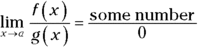, the function has no limit at a.
• If , the function has a limit at a. You reduce the fraction and evaluate the newly formed function equation at a (as I explain how to do in the preceding section).

A fraction has no value when a zero sits in the denominator, but a zero divided by a zero does have a form — called an indeterminate form. Take this form as a signal that you can look for a value for the limit.

For example, here’s a function that has no limit when : You’re looking at what x is approaching in the limit statement, so you’re only concerned about the 1.

The function has no limit at 1 because the substitution creates a number over zero.

If you try this function at , you see that the function has a removable discontinuity:

The function has a limit at because the substitution gives you zero over zero. When you factor out of the numerator and denominator and then evaluate the new fraction for , you get a limit of 3.

Going to infinity

When a rational function doesn’t have a limit at a particular value, the function values and graph have to go somewhere. A particular function may not have the number 3 in its domain, and its graph may have a vertical asymptote when . Even though the function has no limit, you can still say something about what’s happening to the function as it approaches 3 from the left and the right. The graph has no numerical limit at that point, but you can still tell something about the behavior of the function. The behavior is attributed to one-sided limits.

A one-sided limit tells you what a function is doing at an x-value as the function approaches from one side or the other. One-sided limits are more restrictive; they work only from the left or from the right.

The notation for indicating one-sided limits from the left or right is shown here:

• The limit as x approaches the value a from the left is .
• The limit as x approaches the value a from the right is .

Do you see the little positive or negative sign after the a? You can think of from the left as coming from the same direction as all the negative numbers on the number line and from the right as coming from the same direction as all the positive numbers.

Table 9-4 shows some values of the function , which has a vertical asymptote at .

You express the one-sided limits for the function from Table 9-4 as follows:

and

The function goes down to negative infinity as it approaches 3 from less than the value and up to positive infinity as it approaches 3 from greater than the value. “And nary the twain shall meet.”

Catching rational limits at infinity

The previous section describes how function values can go to positive or negative infinity as x approaches some specific number. This section also talks about infinity, but it focuses on what rational functions do as their x-values become very large or very small (approaching infinity themselves).

A function such as the parabola opens upward. If you let x be some really big number, y gets very big, too. Also, when x is very small (a “big” negative number), you square the value, making it positive, so y is very big for the small x. In function notation, you describe what’s happening to this function as the x-values approach infinity with .

You can indicate that a function approaches positive infinity going in one direction and negative infinity going in another direction with the same kind of notation you use for one-sided limits (see the previous section).

For example, the function approaches negative infinity as x gets very large — think about what does to the y value (you’d get ). On the other hand, when , the y value gets very large, because you have , so the function approaches positive infinity.

In the case of rational functions, the limits at infinity — as x gets very large or very small — may be specific, finite, describable numbers. In fact, when a rational function has a horizontal asymptote, its limit at infinity is the same value as the number in the equation of the asymptote.

If you’re looking for the horizontal asymptote of the function , for example, you can use the rules in the section “Determining the equations of horizontal asymptotes” to determine that the horizontal asymptote of the function is . Using limit notation, you can write the solution as .

The proper algebraic method for evaluating limits at infinity is to divide every term in the rational function by the highest power of x in the fraction and then look at each term. Here’s an important property to use: As x approaches infinity, any term with or any positive power of x, , in it approaches zero — in other words, gets very small — so you can replace those terms with zero and simplify.

Here’s how the property works when evaluating the limit of the previous example function, . The highest power of the variable in the fraction is , so every term is divided by :

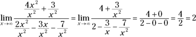
The limit as x approaches infinity is 2. As predicted, the number 2 is the number in the equation of the horizontal asymptote. The quick method for determining horizontal asymptotes is an easier way to find limits at infinity, and this procedure is also the correct mathematical way of doing it — and it shows why the other rule (the quick method) works. You also need this quicker method for more involved limit problems found in calculus and other higher mathematics.