Chapter 13
Solving Systems of Nonlinear Equations and Inequalities
IN THIS CHAPTER
![]() Pinpointing solutions of parabola/line systems
Pinpointing solutions of parabola/line systems
![]() Combining parabolas and circles to find intersections
Combining parabolas and circles to find intersections
![]() Attacking polynomial, exponential, and rational systems
Attacking polynomial, exponential, and rational systems
![]() Exploring the shady world of nonlinear inequalities
Exploring the shady world of nonlinear inequalities
In systems of linear equations, the variables have exponents of 1, and you typically find only one solution (see Chapter 12). The possibilities for multiple solutions in systems seem to grow as the exponents of the equations get larger, creating systems of nonlinear equations. For example, a line and parabola may intersect in two points, at one point, or at no point at all. A circle and ellipse can intersect in four different points. And consider inequalities. The graphs of inequalities involve many solutions. When you put two inequalities together, the possibilities are infinitely exciting (well, at least from my perspective).
One of the most important parts of solving nonlinear systems is planning. If you have an inkling as to what’s coming, you’ll have an easy time planning for the solution, and you’ll be more convinced when your predictions come true. In this chapter, you find out at how many points a line and a parabola can cross and how many ways a parabola and a circle can cross. I also help you visualize a circle and an ellipse — when you put one on top of the other, you can plan on how many points of intersection you expect to find. Finally, you see how graphing inequalities takes on a whole new picture — catching curvy areas between circles and the like.
Crossing Parabolas with Lines
A parabola is a predictable, smooth, U-shaped curve (which I first introduce in detail in Chapter 7). A line is also very predictable; it goes up or down and left or right at the same rate forever and ever. If you put these two characteristics together, you can predict with a fair amount of accuracy what will happen when a line and a parabola share the same place in space.
When you combine the equations of a line and a parabola, you get one of three results (which you can check out in Figure 13-1):
- Two common solutions (Figure 13-1a)
- One common solution (Figure 13-1b)
- No solution at all (Figure 13-1c)

John Wiley & Sons, Inc.
FIGURE 13-1: A line and a parabola sharing space on a graph.
 The easiest way to find the common solutions, or sets of values, for a line and a parabola is to solve their system of equations algebraically. A graph is helpful for confirming your work and putting the problem into perspective. When solving a system of equations involving a line and a parabola, most mathematicians use the substitution method. For a complete look at how to use substitution, refer to Chapter 12. You can also pick up on the method by following the work in the coming pages.
You almost always substitute x’s for the y’s in an equation, because you often see functions written with the y’s equal to so many x’s. You may have to replace x’s with y’s, but that’s the exception. Just be flexible. (If you want to see an exception, check out the “Sorting out the solutions” section later in this chapter.)
Determining the point(s) where a line and parabola cross paths
The graphs of a line and a parabola can cross in two places, one place, or no place at all (see Figure 13-1). In terms of equations, these assertions translate to two common solutions, one solution, or no solution at all. Doesn’t that fit together nicely?
Finding two solutions
The parabola ![]() and the line
and the line ![]() have two points in common. To solve for the two solutions by using the substitution method, you first solve for y in the equation of the line:
have two points in common. To solve for the two solutions by using the substitution method, you first solve for y in the equation of the line: ![]() .
.
Substitute this equivalence of y into the first equation: ![]() . Next, set the new equation equal to zero, and factor as you do any quadratic equation (see Chapter 3):
. Next, set the new equation equal to zero, and factor as you do any quadratic equation (see Chapter 3): ![]() .
.
Setting each of the binomial factors equal to zero, you get ![]() and
and ![]() . When you substitute those values into the equation
. When you substitute those values into the equation ![]() , you find that when
, you find that when ![]() ,
, ![]() , and when
, and when ![]() ,
, ![]() . The two points of intersection, therefore, are (2, 3) and
. The two points of intersection, therefore, are (2, 3) and ![]() . Figure 13-2 shows the graphs of the parabola
. Figure 13-2 shows the graphs of the parabola ![]() , the line
, the line ![]() , and the two points of intersection.
, and the two points of intersection.

John Wiley & Sons, Inc.
FIGURE 13-2: You find the two points of intersection with substitution.
Settling for one solution
When a line and a parabola have one point of intersection, and their equations share one common solution, the line is tangent to the parabola. A line and a curve can be tangent to one another if they touch or share exactly one point and if the line appears to follow the curvature at that point. (Two curves can also be tangent to one another — they touch at a point and then go their own merry ways.) The parabola ![]() and the line
and the line ![]() , for example, have only one point in common — at their point of tangency. Figure 13-3 shows how a line and a parabola can be tangent.
, for example, have only one point in common — at their point of tangency. Figure 13-3 shows how a line and a parabola can be tangent.

John Wiley & Sons, Inc.
FIGURE 13-3: The line touches the parabola in just one place — at their point of tangency.
You find the coordinate of the point that the parabola and line share by solving the system of equations formed by the parabola and line. You substitute the equivalence of y in the line equation into the parabolic equation and solve for x (see Chapter 12): ![]() is set equal to 0, giving you
is set equal to 0, giving you ![]() . Factor out
. Factor out ![]() , and then factor the trinomial:
, and then factor the trinomial: ![]() . Setting the binomial
. Setting the binomial ![]() , you have
, you have ![]() , which is the only solution.
, which is the only solution.
 The dead giveaway that the parabola and line are tangent is the quadratic equation that results from the substitution. It has a double root — the same solution appears twice — when the binomial factor is squared.
Substituting ![]() into the equation of the line, you get
into the equation of the line, you get ![]() . The coordinates of the point of tangency are (1, 10).
. The coordinates of the point of tangency are (1, 10).
Dealing with a solution that’s no solution
You can see when no solution exists in a system of equations involving a parabola and line if you graph the two figures and find that their paths never cross. You also discover that a parabola and line don’t intersect when you get a no-answer answer to the algebra problem — no need to even graph the figures. For instance, if you solve the system of equations containing the parabola ![]() and the line
and the line ![]() by using substitution (see Chapter 12), you first replace all the y’s in the equation of the parabola with
by using substitution (see Chapter 12), you first replace all the y’s in the equation of the parabola with ![]() . Square the binomial and distribute the
. Square the binomial and distribute the ![]() to get
to get ![]() . When you simplify on the right and set the equation equal to 0, the equation becomes
. When you simplify on the right and set the equation equal to 0, the equation becomes ![]() . The equation looks perfectly good so far, even though the quadratic doesn’t factor. You have to resort to the quadratic formula. (You can find details on using the quadratic formula in Chapter 3, if you need a refresher.) Substituting the numbers from the quadratic equation into the formula, you get the following:
. The equation looks perfectly good so far, even though the quadratic doesn’t factor. You have to resort to the quadratic formula. (You can find details on using the quadratic formula in Chapter 3, if you need a refresher.) Substituting the numbers from the quadratic equation into the formula, you get the following:
Whoa! You can stop right there. You see that a negative value sits under the radical. The square root of ![]() isn’t real, so no real answer exists for x (for more on nonreal numbers, see Chapter 14). The nonexistent answer is your big clue that the system of equations doesn’t have a common solution, meaning that the parabola and line never intersect (hey, even Sherlock Holmes had to dig around a bit before finding his clue). Figure 13-4 shows the graphs of the parabola and line. You can see why you found no solution. I wish I could give you an easy way to tell that a system has no solution before you go to all that work. Think of it this way: An answer of no solution is a perfectly good answer.
isn’t real, so no real answer exists for x (for more on nonreal numbers, see Chapter 14). The nonexistent answer is your big clue that the system of equations doesn’t have a common solution, meaning that the parabola and line never intersect (hey, even Sherlock Holmes had to dig around a bit before finding his clue). Figure 13-4 shows the graphs of the parabola and line. You can see why you found no solution. I wish I could give you an easy way to tell that a system has no solution before you go to all that work. Think of it this way: An answer of no solution is a perfectly good answer.

John Wiley & Sons, Inc.
FIGURE 13-4: The algebra shows that ne’er the twain shall meet.
Intertwining Parabolas and Circles
The graph of a parabola is a U-shaped curve, and a circle — well, you could go round and round about a circle. When a parabola and circle share the same gridded plot, they can interact in several different ways (much like you and your neighbors, I suppose). The figures can intersect at four different points, three points, two points, one point, or no points at all. The possibilities may seem endless, but that’s wishful thinking. The five possibilities I list here are what you have to work with. Your challenge is to determine which situation you have and to find the solutions of the system of equations (not as challenging as getting your neighbor to return borrowed items, you’ll be glad to know).
Managing multiple intersections
A parabola and a circle can intersect at up to four different points, meaning that their equations can have up to four common solutions. Figure 13-5 shows just such a situation.

John Wiley & Sons, Inc.
FIGURE 13-5: A parabola and circle intersecting at four points.
To solve for the common solutions you see in Figure 13-5, you have to solve the system of equations that includes ![]() , the equation of a parabola, and
, the equation of a parabola, and ![]() , the equation of a circle. Here are the steps for solving this system:
, the equation of a circle. Here are the steps for solving this system:
If the parabola and the circle don’t appear in their standard forms, you should get them there if you want to graph them.
In this case, you need to change the circle to its standard form —
 — by completing the square (see Chapter 11). The circle’s equation, written in standard form, is
  . (For more on the parabola’s standard form, check out Chapters 3 and 7.)
To solve for common points, replace each y in the equation of the circle with the equivalence of y in the parabola.
Starting with the general form
 (not the standard form you use to graph the circle), replace each y with
  . This process requires squaring a trinomial, unfortunately.
When squaring a trinomial, you may find it easier to distribute the terms instead of stacking the terms like in a multiplication problem. To find
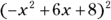 , for example, think of the product
  . You multiply each term by
  , and then by 6x, and lastly by 8. Finish by combining the like terms (see Chapter 8 for more on polynomials):
Set the resulting terms from Step 2 equal to zero and solve for x (this usually requires factoring or the use of the quadratic formula; see Chapter 3).
The terms in the equation have a common factor of x. Factoring out the x, you get
 . The expression in the parentheses factors into the product of three binomials. You can do this factorization and find these binomials by using the Rational Root Theorem, which leads you to try the factors of 42 — 1, 6, and 7 — and synthetic division. (Chapter 8 has a full explanation of the Rational Root Theorem and factoring.) The final factorization of the equation is
  . The solutions are
  , 6, and 7.
Substitute the solutions you find into the equation of the curve with the smaller exponents to find the coordinates of the points of intersection.
In this case, you substitute into the equation of the parabola. You find that when
 ,
,  ; when
  ,
,  ; when
  ,
,  ; and when
  ,
,  . The points of intersection are, therefore, (0, 8),
  , (6, 8), and (7, 1). Refer to Figure 13-5 for a graph of the parabola, circle, and points of intersection.
A circle and a parabola can also intersect at three points, two points, one point, or no points. Figure 13-6 shows what the three-point and two-point situations look like. In Figure 13-6a, the parabola’s vertex is tangent to a point on the circle, and the parabola cuts the circle at two other points. In Figure 13-6b, the parabola cuts the circle at only two points.

John Wiley & Sons, Inc.
FIGURE 13-6: Parabolas and circles tangling, offering up different solutions.
 You use the same substitution method to solve systems of equations with fewer than four intersections. The algebra leads you to the solutions — but beware the false promises. You have to watch out for extraneous solutions by checking your answers.
After substituting one equation into another, take a look at the resulting equation. The highest power of the equation tells you what to expect as far as the number of common solutions. When the power is three or four, you can have as many as three or four solutions, respectively (see Chapter 8 on solving polynomials). When the power is two, you can have up to two common solutions (Chapter 3 covers these equations). A power of one indicates only one possible solution (see Chapter 2). If you end up with an equation that has no solutions, you know the system has no points of intersection — the graphs just pass by like ships in the night.
Sorting out the solutions
In the section “Crossing Parabolas with Lines” earlier in the chapter, the examples I provide use substitution where the x’s replace the y variable. Most of the time, this is the method of choice, but I suggest you remain flexible and open for other opportunities. The next example is just such an opportunity — taking advantage of a situation where it makes more sense to replace the x term with the y term.
To find the common solutions of the parabola ![]() , which has its vertex at the origin (see Chapter 7), and the circle
, which has its vertex at the origin (see Chapter 7), and the circle ![]() , which has its center at (0, 1) and has a radius of 3 (see Chapter 11), you take advantage of the simplicity of
, which has its center at (0, 1) and has a radius of 3 (see Chapter 11), you take advantage of the simplicity of ![]() by replacing the
by replacing the ![]() in the circle equation with y. That sets you up with an equation of y’s to solve. Replacing the
in the circle equation with y. That sets you up with an equation of y’s to solve. Replacing the ![]() term, you have
term, you have ![]() . Square the binomial and combine like terms to get
. Square the binomial and combine like terms to get ![]() , which simplifies to
, which simplifies to ![]() . This quadratic equation doesn’t factor, so you have to use the quadratic formula (see Chapter 3) to solve for y:
. This quadratic equation doesn’t factor, so you have to use the quadratic formula (see Chapter 3) to solve for y:
You find two different values for y, according to this solution. When you use the positive part of the ![]() , you find that y is close to 3.37. When you use the negative part, you find that y is about
, you find that y is close to 3.37. When you use the negative part, you find that y is about ![]() . Something doesn’t seem right. What is it that’s bothering you? It has to be the negative value for y. The common solutions of a system should work in both equations, and
. Something doesn’t seem right. What is it that’s bothering you? It has to be the negative value for y. The common solutions of a system should work in both equations, and ![]() doesn’t work in
doesn’t work in ![]() , because when you square x, you don’t get a negative number. So, only the positive part of the solution, where
, because when you square x, you don’t get a negative number. So, only the positive part of the solution, where ![]() , works.
, works.
Substitute ![]() into the equation
into the equation ![]() to get x. If
to get x. If ![]() , then, taking the square root of both sides,
, then, taking the square root of both sides, ![]() . The value of x comes out to about
. The value of x comes out to about ![]() . The graph in Figure 13-7 shows you the parabola, the circle, and the points of intersection at about (1.84, 3.37) and about
. The graph in Figure 13-7 shows you the parabola, the circle, and the points of intersection at about (1.84, 3.37) and about ![]() .
.

John Wiley & Sons, Inc.
FIGURE 13-7: This system has only two points of intersection.
When ![]() , you get points that lie on the circle, but these points don’t fall on the parabola. The algebra shows that, and the picture agrees.
, you get points that lie on the circle, but these points don’t fall on the parabola. The algebra shows that, and the picture agrees.
When substituting into one of the original equations to solve for the other variable, always substitute into the simpler equation — the one with smaller exponents. This helps you catch any extraneous solutions.
Planning Your Attack on Other Systems of Equations
I deal with intersections of lines and different conic sections first in this chapter because the curves of the conics are easy to visualize and the results of the intersections are somewhat predictable. However, you can also find the intersections (common solutions) of other functions and curves; you may just have to start out with no clue as to what’s going to happen. Not to worry, though; using the correct processes — substitution and equation solving (see Chapter 12) — assures you of honest answers and results.
You can deal with a system of linear equations in many ways. (I cover the methods for solving systems of linear equations in great detail in Chapter 12.) A system of equations that contains one or more polynomial (nonlinear) functions, however, presents fewer options for finding the solutions. Throw in a rational function or exponential function, and the plot thickens. But as long as the equations cooperate, the different algebraic methods — elimination and substitution — will work. Lucky you!
 Cooperative equations are the ones I discuss in this book. When systems of equations defy algebraic methods, you have to turn to calculators, computers, and high-powered college mathematics courses. In the meantime, you can concentrate on the nicely defined, manageable systems I present in this section for nonlinear entities.
Mixing polynomials and lines
A polynomial is a continuous, smooth curve. (Chapter 8 gives you plenty of information on the behavior of polynomial curves and how to graph them.) The more the curve of a polynomial changes direction and moves up and down across a graph, the more opportunities a line has to cross it. For instance, the line ![]() intersects the polynomial
intersects the polynomial ![]() three times. Figure 13-8 shows you the graphs of the line, the polynomial, and the points of intersection.
three times. Figure 13-8 shows you the graphs of the line, the polynomial, and the points of intersection.

FIGURE 13-8: A line crossing the curves of a polynomial.
Substitution that replaces the y in the polynomial with the equivalence of y in the line is usually your most effective route for solving for the common solutions of the intersections. ( You apply this method when the solutions are cooperative integers. If the common points involve fractions and radicals, technology is the only way to go.)
To solve for the solutions of this system of equations by using substitution, you start by replacing the y in the polynomial with the equivalence of y in the line: ![]() becomes
becomes ![]() . Move the terms to the left to set the equation equal to
. Move the terms to the left to set the equation equal to ![]() . This result factors into
. This result factors into ![]() . (If you need help with this factorization, refer to the Rational Root Theorem and synthetic division information in Chapter 8.) The zeros, or solutions, of the equation are
. (If you need help with this factorization, refer to the Rational Root Theorem and synthetic division information in Chapter 8.) The zeros, or solutions, of the equation are ![]() . You solve for the y-values of the intersection points by plugging these x-values into the equation of the line. The points of intersection that you find are
. You solve for the y-values of the intersection points by plugging these x-values into the equation of the line. The points of intersection that you find are ![]() , (1, 24), and (7, 42).
, (1, 24), and (7, 42).
Always use the equation with the smaller exponents when you solve for the full solution. The substitution is easier with smaller exponents, and, more importantly, you won’t end up with extraneous solutions — nonexistent answers for the problem (for more on imaginary numbers, see Chapter 14).
Crossing polynomials
“Crossing polynomials” almost sounds like you’re doing a genetics experiment and creating a new, hybrid curve — a nonlinear monster of sorts. But before I start my sinister laugh, I must admit that crossing polynomials is bloomin’ wonderful stuff. (Hey, beauty is in the eye of the beholder.)
Just to give you an example of how intersecting polynomials can provide several solutions, I’ve chosen a quartic and a cubic to cross-pollinate (oops, I mean intersect). A fourth-degree (quartic) polynomial (the power 4 is the highest power) and a third-degree (cubic) polynomial can share as many as four common solutions. The graphs of ![]() and
and ![]() , for example, are shown in Figure 13-9. The W-shaped curve is the fourth-degree polynomial, and the sideways S is the third-degree polynomial.
, for example, are shown in Figure 13-9. The W-shaped curve is the fourth-degree polynomial, and the sideways S is the third-degree polynomial.

John Wiley & Sons, Inc.
FIGURE 13-9: Counting the intersections of quartic and cubic polynomials.
To solve systems of equations containing two polynomials, you use the substitution method (see Chapter 12). Set y equal to y, move all the terms to the left, and simplify: ![]() becomes
becomes ![]() .
.
This equation factors into ![]() (see Chapter 8), which gives you the solutions
(see Chapter 8), which gives you the solutions ![]() , and 4. Substituting these values into the cubic (third-degree) equation (you should always substitute into the equation with the smallest exponential values), you get
, and 4. Substituting these values into the cubic (third-degree) equation (you should always substitute into the equation with the smallest exponential values), you get ![]() when
when ![]() ,
, ![]() when
when ![]() ,
, ![]() when
when ![]() , and
, and ![]() when
when ![]() . You now have all the points of intersection.
. You now have all the points of intersection.
Navigating exponential intersections
Exponential functions are flattened, C-shaped curves when graphed (I cover exponentials in Chapter 10). When exponentials intersect with one another, they usually do so in only one place, creating one common solution. Mixing exponential curves with other types of curves produces results similar to those you see when mixing lines and parabolas — you may get more than one solution.
Visualizing exponential solutions
The exponential functions ![]() and
and ![]() have one common solution: They both cross the y-axis at the point (0, 1). If you let
have one common solution: They both cross the y-axis at the point (0, 1). If you let ![]() in
in ![]() , you get
, you get ![]() . Anything to the zero power equals one. So, that means substituting 0 for x in
. Anything to the zero power equals one. So, that means substituting 0 for x in ![]() gives you
gives you ![]() . You get the same number for both equations. You know (0, 1) is the only possible solution for the two exponential functions because any other power of 5 and 3 won’t give you the same number. The numbers 3 and 5 are both prime numbers, and raising them to powers won’t create any common solutions. You can discover the solution through algebra, through reasoning it out, or by looking at the graphs of the equations. The graphs of the exponential functions
. You get the same number for both equations. You know (0, 1) is the only possible solution for the two exponential functions because any other power of 5 and 3 won’t give you the same number. The numbers 3 and 5 are both prime numbers, and raising them to powers won’t create any common solutions. You can discover the solution through algebra, through reasoning it out, or by looking at the graphs of the equations. The graphs of the exponential functions ![]() and
and ![]() are shown in Figure 13-10a. The steeper of the two exponential curves is
are shown in Figure 13-10a. The steeper of the two exponential curves is ![]() .
.

John Wiley & Sons, Inc.
FIGURE 13-10: Graphing systems containing exponential equations.
Figure 13-10b shows the intersections of the line ![]() and the exponential function
and the exponential function ![]() . Due to the complexities of the exponential function, it isn’t practical to solve this system of equations algebraically. It’s time to get some help from technology. But, if you can determine the solutions by looking at the graphs, take advantage of the situation. The two solutions that the line and exponential function appear to have in common — where they intersect — are at
. Due to the complexities of the exponential function, it isn’t practical to solve this system of equations algebraically. It’s time to get some help from technology. But, if you can determine the solutions by looking at the graphs, take advantage of the situation. The two solutions that the line and exponential function appear to have in common — where they intersect — are at ![]() and (0, 2), assuming that each notch on each axis moves one unit at a time (you expect only two solutions because the line keeps going on in one direction, and the exponential function just keeps growing, like exponential functions do, and doesn’t double back on itself). You can check to be sure that these answers are correct by substituting the x-values into the equations to see if you get the correct y-values:
and (0, 2), assuming that each notch on each axis moves one unit at a time (you expect only two solutions because the line keeps going on in one direction, and the exponential function just keeps growing, like exponential functions do, and doesn’t double back on itself). You can check to be sure that these answers are correct by substituting the x-values into the equations to see if you get the correct y-values:
- When
 in the equation of the line,
  .
. - When
 in the equation of the exponential, you get the following:
- The line and the exponential have the common solution
 .
. - When
 in the equation of the line,
 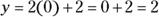 .
. - When
 in the equation of the exponential, you get the following:
  .
. - The line and the exponential have the common solution (0, 2).
Solving for exponential solutions
You can solve some systems that contain exponential functions by using algebraic techniques. What should you look for? When the bases of the exponential functions are the same number or are powers of the same number, an algebraically found solution is possible.
For instance, you can solve the system ![]() and
and ![]() algebraically because the base 4 in the first equation is a power of 2, the base in the second equation. You can write the number 4 as
algebraically because the base 4 in the first equation is a power of 2, the base in the second equation. You can write the number 4 as ![]() . (If you need a refresher on dealing with exponential equations, head to Chapter 10.)
. (If you need a refresher on dealing with exponential equations, head to Chapter 10.)
 To solve a system of exponential functions when the bases of the functions are the same number or are powers of the same number, you set the two y-values equal to one another, set the exponents equal to one another, and solve for x. You change it from the exponential form by setting those exponents equal to one another and discarding the bases.
Setting the two y-values equal to one another for the previous example, you have

Now you can set the exponents equal to one another. The solution of ![]() is
is ![]() . When
. When ![]() ,
, ![]() in both equations. Figure 13-11 shows the graphs of the intersecting curves.
in both equations. Figure 13-11 shows the graphs of the intersecting curves.

John Wiley & Sons, Inc.
FIGURE 13-11: Two exponential functions intersecting at (1, 4).
Rounding up rational functions
A rational function is a fraction that contains a polynomial expression in both its numerator and denominator. A polynomial has one or more terms that have whole-number exponents, so a rational function has all whole-number exponents — just in fractional form. The graph of a rational function typically has vertical and/or horizontal asymptotes that reveal its shape. Also, rational functions usually have pieces of curves that resemble hyperbolas in their graphs. (You can find plenty of information on rational functions in Chapter 9.)
Solving and graphing systems of equations that include rational functions means dealing with fractions — every student and teacher’s favorite task. No worries, though. I prepare you in the following sections.
Intersections of a rational function and a line
The rational function ![]() and the line
and the line ![]() intersect at two points, meaning they have two common solutions. You can see that from their graphs in Figure 13-12. But don’t confuse the intersections of the line with the asymptotes of the rational function as parts of the solution. You consider only the intersections with the curves of the rational function. The algebraic solution you find also confirms that you use only the points on the curve.
intersect at two points, meaning they have two common solutions. You can see that from their graphs in Figure 13-12. But don’t confuse the intersections of the line with the asymptotes of the rational function as parts of the solution. You consider only the intersections with the curves of the rational function. The algebraic solution you find also confirms that you use only the points on the curve.

John Wiley & Sons, Inc.
FIGURE 13-12: A line crossing a rational function, forming two solutions.
To solve this system of equations, you solve the equation of the line for y, and then you substitute this equivalence for y into the equation of the rational function. First solving for y in the line, you get ![]() and then
and then ![]() . Setting y equal to y, you get
. Setting y equal to y, you get
The equation that remains looks like a bit of a mess, doesn’t it? You can make the equation look much nicer by multiplying each side by ![]() , the common denominator of the fractions in the equation:
, the common denominator of the fractions in the equation:
Now you can simplify the resulting equation by distributing and combining like terms (see Chapter 1 to find out how): ![]() becomes
becomes ![]() . Now set the whole equation equal to zero:
. Now set the whole equation equal to zero: ![]() . The result is a quadratic equation that you can factor (see Chapter 3):
. The result is a quadratic equation that you can factor (see Chapter 3): ![]() .
.
When you change the form of an equation that contains fractions, radicals, or exponentials, you have to be cautious about extraneous solutions — answers that satisfy the new form but not the original. Always check your work by substituting your answers into the original equation.
The solutions of the quadratic equation are ![]() and
and ![]() . You now substitute these values into the rational function to check your work. When
. You now substitute these values into the rational function to check your work. When ![]() , you get
, you get ![]() . When
. When ![]() , you get
, you get ![]() . These values represent the common solutions (coordinates of intersection) of the rational function and the line (you can see them in Figure 13-12).
. These values represent the common solutions (coordinates of intersection) of the rational function and the line (you can see them in Figure 13-12).
Discovering that functions are inverses when solving a system
With a little algebra and graphing, you’ll notice something special about the two rational functions in the following system:

When you solve the system by identifying the solutions, you notice something that may or may not be a coincidence. A graph helps confirm that your discovery isn’t a coincidence. Okay, enough with the suspense. To solve the system, you set the two fractions equal to one another — the same as substituting the y equivalences for one another:
The equation you create is a proportion, meaning that you have two different ratios (fractions) set equal to one another. Cross-multiply and simplify the products, and then move every term over to the left to set the equation equal to zero: ![]() becomes
becomes ![]() . Moving the terms to the left, you have
. Moving the terms to the left, you have ![]() . The quadratic equation factors into
. The quadratic equation factors into ![]() , so the two solutions are
, so the two solutions are ![]() and
and ![]() . You substitute those values into either of the original equations. You find that when
. You substitute those values into either of the original equations. You find that when ![]() ,
, ![]() , and when
, and when ![]() ,
, ![]() .
.
So, back to the big mystery. Do you notice anything special about these values? Yep, the x and y-values are the same, because they both lie on the line ![]() . This phenomenon happens because the two rational functions are inverses of one another. (You can find more on function inverses in Chapter 6.)
. This phenomenon happens because the two rational functions are inverses of one another. (You can find more on function inverses in Chapter 6.)
The special characteristic about the graphs of functions and their inverses is that they’re always symmetric with respect to one another over the line ![]() . Also, if they intersect that line of symmetry, they intersect in the same place, making for a rather artsy picture. Figure 13-13 shows the two rational functions I previously introduce and how they’re symmetric about the line
. Also, if they intersect that line of symmetry, they intersect in the same place, making for a rather artsy picture. Figure 13-13 shows the two rational functions I previously introduce and how they’re symmetric about the line ![]() . (I leave out the lines showing the asymptotes so the picture doesn’t get too cluttered.)
. (I leave out the lines showing the asymptotes so the picture doesn’t get too cluttered.)

John Wiley & Sons, Inc.
FIGURE 13-13: Two inverse rational functions reflected over the line  .
.
Playing Fair with Inequalities
Systems of inequalities appear in applications used for business ventures and calculus problems. A system of inequalities, for instance, can represent a set of constraints in a problem that involves production of some item — the constraints put limits on the resources being used or the time available. In calculus, systems of inequalities represent areas between curves that you need to compute. Graphically, the solutions of systems of inequalities appear as shaded areas between curves. This gives you a visual solution and helps you determine values of x and y that work.
You find so many answers for systems of inequalities — infinitely many solutions — that you can’t list them all; you just give rules in terms of the inequality statements. Algebraically, the solutions are statements that involve inequalities — telling what x or y is bigger than or smaller than. Often, the graph of a system gives you more information than the listing of the inequalities shown in an algebraic solution. You can see that all the points in the solution lie above a certain line, so you pick numbers that work in the system based on what you see.
Drawing and quartering inequalities
The simplest inequality to graph and solve is one that falls above or below a horizontal line or to the right or left of a vertical line. A system of inequalities that involves two such lines (one vertical and one horizontal) has a graph that appears as one quarter of the plane. For instance, the graph of the system of inequalities ![]() is shown in Figure 13-14.
is shown in Figure 13-14.
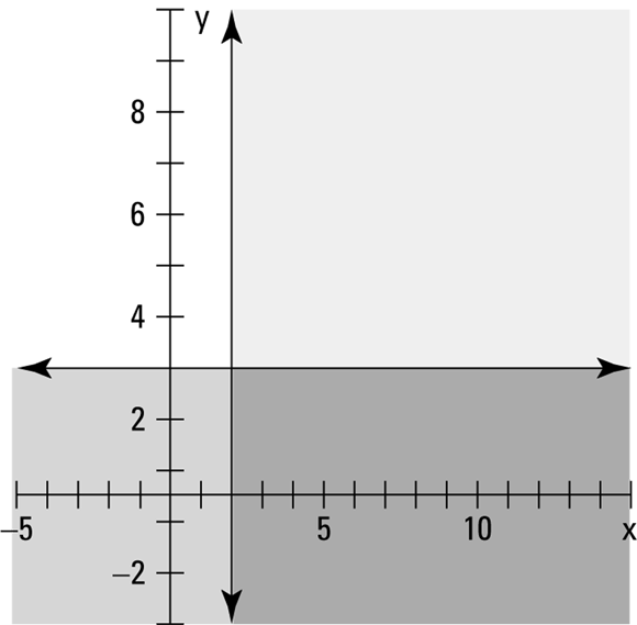
John Wiley & Sons, Inc.
FIGURE 13-14: Two inequalities intersecting to share a portion of the plane (the heavy shading).
Everything to the right of the line ![]() represents the graph of
represents the graph of ![]() , and everything below the line
, and everything below the line ![]() represents the graph of
represents the graph of ![]() . Their intersection, the heavily shaded area in the lower-right quadrant formed by the intersecting lines, consists of all the points in that shaded area. You can find an infinite number of solutions. Some examples are the points (3, 1), (4, 2), and
. Their intersection, the heavily shaded area in the lower-right quadrant formed by the intersecting lines, consists of all the points in that shaded area. You can find an infinite number of solutions. Some examples are the points (3, 1), (4, 2), and ![]() . You could never list all the answers.
. You could never list all the answers.
Graphing areas with curves and lines
You find the solution of a system of inequalities involving a line and a curve (such as a parabola), two curves, or any other such combination by graphing the individual equations, determining which side to shade for each curve, and identifying where the equations share the shading.
To solve the system ![]() , for example, make your way through the following steps:
, for example, make your way through the following steps:
Graph the line
 and determine which side of the line to shade by checking a test point (a random point that’s clearly on one side or the other) to see if it satisfies the inequality. (For info on graphing lines, see Chapters 2 and 5.)
If the point satisfies the inequality, you shade that side. In this case, you can use the test point (0, 0), which is clearly above and to the left of the line. When you put the coordinate (0, 0) in the inequality
 , you get
  . Yes, 0 is greater than
  , so the test point is in the area that you need to shade — above the line.
Graph the parabola
 and use a test point to see whether you need to shade inside the parabola or outside the parabola. (For info on graphing parabolas, see Chapters 5 and 7.)
Again, the point (0, 0) is handy. Test the point in the inequality for the parabola,
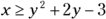 . You find
  , which is true. So, the point (0, 0) falls in the area you need to shade — inside the parabola.
Determine where the two shaded areas overlap to find your solution to the system of inequalities.
The two shaded areas overlap where the inside of the parabola and area above the line intersect.
Figure 13-15 shows the line and parabola corresponding to the inequalities. The shaded area indicates the solution — where the two inequalities overlap.
John Wiley & Sons, Inc.
FIGURE 13-15: A parabola and line outline a solution wedge for the inequalities.