
Chapter Six. Elementary Sorting Methods
For our first excursion into the area of sorting algorithms, we shall study several elementary methods that are appropriate for small files, or for files that have a special structure. There are several reasons for studying these simple sorting algorithms in detail. First, they provide context in which we can learn terminology and basic mechanisms for sorting algorithms, and thus allow us to develop an adequate background for studying the more sophisticated algorithms. Second, these simple methods are actually more effective than the more powerful general-purpose methods in many applications of sorting. Third, several of the simple methods extend to better general-purpose methods or are useful in improving the efficiency of more sophisticated methods.
Our purpose in this chapter is not just to introduce the elementary methods, but also to develop a framework within which we can study sorting in later chapters. We shall look at a variety of situations that may be important in applying sorting algorithms, examine different kinds of input files, and look at other ways of comparing sorting methods and learning their properties.
We begin by looking at a simple driver program for testing sorting methods, which provides a context for us to consider the conventions that we shall follow. We also consider the basic properties of sorting methods that are important for us to know when we are evaluating the utility of algorithms for particular applications. Then, we look closely at implementations of three elementary methods: selection sort, insertion sort, and bubble sort. Following that, we examine the performance characteristics of these algorithms in detail. Next, we look at shellsort, which is perhaps not properly characterized as elementary, but is easy to implement and is closely related to insertion sort. After a digression into the mathematical properties of shellsort, we delve into the subject of developing data type interfaces and implementations, along the lines that we have discussed in Chapters 3 and 4, for extending our algorithms to sort the kinds of data files that arise in practice. We then consider sorting methods that refer indirectly to the data and linked-list sorting. The chapter concludes with a discussion of a specialized method that is appropriate when the key values are known to be restricted to a small range.
In numerous sorting applications, a simple algorithm may be the method of choice. First, we often use a sorting program only once, or just a few times. Once we have “solved” a sort problem for a set of data, we may not need the sort program again in the application manipulating those data. If an elementary sort is no slower than some other part of processing the data—for example reading them in or printing them out—then there may be no point in looking for a faster way. If the number of items to be sorted is not too large (say, less than a few hundred elements), we might just choose to implement and run a simple method, rather than bothering with the interface to a system sort or with implementing and debugging a complicated method. Second, elementary methods are always suitable for small files (say, less than a few dozen elements)—sophisticated algorithms generally incur overhead that makes them slower than elementary ones for small files. This issue is not worth considering unless we wish to sort a huge number of small files, but applications with such a requirement are not unusual. Other types of files that are relatively easy to sort are ones that are already almost sorted (or already are sorted!) or ones that contain large numbers of duplicate keys. We shall see that several of the simple methods are particularly efficient when sorting such well-structured files.
As a rule, the elementary methods that we discuss here take time proportional to N2 to sort N randomly arranged items. If N is small, this running time may be perfectly adequate. As just mentioned, the methods are likely to be even faster than more sophisticated methods for tiny files and in other special situations. But the methods that we discuss in this chapter are not suitable for large, randomly arranged files, because the running time will become excessive even on the fastest computers. A notable exception is shellsort (see Section 6.6), which takes many fewer than N2 steps for large N, and is arguably the sorting method of choice for midsize files and for a few other special applications.
6.1 Rules of the Game
Before considering specific algorithms, we will find it useful to discuss general terminology and basic assumptions for sorting algorithms. We shall be considering methods of sorting files of items containing keys. All these concepts are natural abstractions in modern programming environments. The keys, which are only part (often a small part) of the items, are used to control the sort. The objective of the sorting method is to rearrange the items such that their keys are ordered according to some well-defined ordering rule (usually numerical or alphabetical order). Specific characteristics of the keys and the items can vary widely across applications, but the abstract notion of putting keys and associated information into order is what characterizes the sorting problem.
If the file to be sorted will fit into memory, then the sorting method is called internal. Sorting files from tape or disk is called external sorting. The main difference between the two is that an internal sort can access any item easily whereas an external sort must access items sequentially, or at least in large blocks. We shall look at a few external sorts in Chapter 11, but most of the algorithms that we consider are internal sorts.
We shall consider both arrays and linked lists. The problem of sorting arrays and the problem of sorting linked lists are both of interest: during the development of our algorithms, we shall also encounter some basic tasks that are best suited for sequential allocation, and other tasks that are best suited for linked allocation. Some of the classical methods are sufficiently abstract that they can be implemented efficiently for either arrays or linked lists; others are particularly well suited to one or the other. Other types of access restrictions are also sometimes of interest.
We begin by focusing on array sorting. Program 6.1 illustrates many of the conventions that we shall use in our implementations. It consists of a driver program that fills an array by reading integers from standard input or generating random ones (as dictated by an integer argument); then calls a sort function to put the integers in the array in order; then prints out the sorted result.
As we know from Chapters 3 and 4, there are numerous mechanisms available to us to arrange for our sort implementations to be useful for other types of data. We shall discuss the use of such mechanisms in detail in Section 6.7. The sort function in Program 6.1 uses a simple inline data type like the one discussed in Section 4.1, referring to the items being sorted only through its arguments and a few simple operations on the data. As usual, this approach allows us to use the same code to sort other types of items. For example, if the code for generating, storing, and printing random keys in the function main in Program 6.1 were changed to process floating-point numbers instead of integers, the only change that we would have to make outside of main is to change the typedef for Item from int to float (and we would not have to change sort at all). To provide such flexibility (while at the same time explicitly identifying those variables that hold items) our sort implementations will leave the data type of the items to be sorted unspecified as Item. For the moment, we can think of Item as int or float; in Section 6.7, we shall consider in detail data-type implementations that allow us to use our sort implementations for arbitrary items with floating-point numbers, strings, and other different types of keys, using mechanisms discussed in Chapters 3 and 4.
We can substitute for sort any of the array-sort implementations from this chapter, or from Chapters 7 through 10. They all assume that items of type Item are to be sorted, and they all take three arguments: the array, and the left and right bounds of the subarray to be sorted. They also all use less to compare keys in items and exch to exchange items (or the compexch combination). To differentiate sorting methods, we give our various sort routines different names. It is a simple matter to rename one of them, to change the driver, or to use function pointers to switch algorithms in a client program such as Program 6.1 without having to change any code in the sort implementation.
These conventions will allow us to examine natural and concise implementations of many array-sorting algorithms. In Sections 6.7 and 6.8, we shall consider a driver that illustrates how to use the implementations in more general contexts, and numerous data type implementations. Although we are ever mindful of such packaging considerations, our focus will be on algorithmic issues, to which we now turn.
The example sort function in Program 6.1 is a variant of insertion sort, which we shall consider in detail in Section 6.3. Because it uses only compare–exchange operations, it is an example of a nonadaptive sort: The sequence of operations that it performs is independent of the order of the data. By contrast, an adaptive sort is one that performs different sequences of operations, depending on the outcomes of comparisons (less operations). Nonadaptive sorts are interesting because they are well suited for hardware implementation (see Chapter 11), but most of the general-purpose sorts that we consider are adaptive.
As usual, the primary performance parameter of interest is the running time of our sorting algorithms. The selection-sort, insertion-sort, and bubble-sort methods that we discuss in Sections 6.2 through 6.4 all require time proportional to N2 to sort N items, as discussed in Section 6.5. The more advanced methods that we discuss in Chapters 7 through 10 can sort N items in time proportional to N log N, but they are not always as good as the methods considered here for small N and in certain other special situations. In Section 6.6, we shall look at a more advanced method (shellsort) that can run in time proportional to N3/2 or less, and, in Section 6.10, we shall see a specialized method (key-indexed sorting) that runs in time proportional to N for certain types of keys.
The analytic results described in the previous paragraph all follow from enumerating the basic operations (comparisons and exchanges) that the algorithms perform. As discussed in Section 2.2, we also must consider the costs of the operations, and we generally find it worthwhile to focus on the most frequently executed operations (the inner loop of the algorithm). Our goal is to develop efficient and reasonable implementations of efficient algorithms. In pursuit of this goal, we will not just avoid gratuitous additions to inner loops, but also look for ways to remove instructions from inner loops when possible. Generally, the best way to reduce costs in an application is to switch to a more efficient algorithm; the second best way is to tighten the inner loop. We shall consider both options in detail for sorting algorithms.
The amount of extra memory used by a sorting algorithm is the second important factor that we shall consider. Basically, the methods divide into three types: those that sort in place and use no extra memory except perhaps for a small stack or table; those that use a linked-list representation or otherwise refer to data through pointers or array indices, and so need extra memory for N pointers or indices; and those that need enough extra memory to hold another copy of the array to be sorted.
We frequently use sorting methods for items with multiple keys—we may even need to sort one set of items using different keys at different times. In such cases, it may be important for us to be aware whether or not the sorting method that we use has the following property:
Definition 6.1 A sorting method is said to be stable if it preserves the relative order of items with duplicated keys in the file.
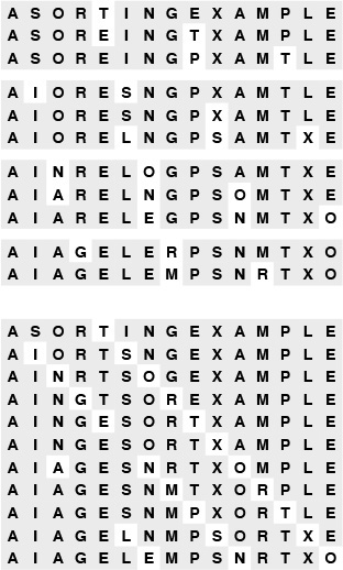
For example, if an alphabetized list of students and their year of graduation is sorted by year, a stable method produces a list in which people in the same class are still in alphabetical order, but a nonstable method is likely to produce a list with no vestige of the original alphabetic order. Figure 6.1 shows an example. Often, people who are unfamiliar with stability are surprised by the way an unstable algorithm seems to scramble the data when they first encounter the situation.
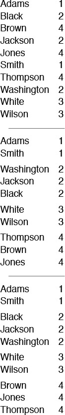
A sort of these records might be appropriate on either key. Suppose that they are sorted initially by the first key (top). A nonstable sort on the second key does not preserve the order in records with duplicate keys (center), but a stable sort does preserve the order (bottom).
Figure 6.1 Stable-sort example
Several (but not all) of the simple sorting methods that we consider in this chapter are stable. On the other hand, many (but not all) of the sophisticated algorithms that we consider in the next several chapters are not. If stability is vital, we can force it by appending a small index to each key before sorting or by lengthening the sort key in some other way. Doing this extra work is tantamount to using both keys for the sort in Figure 6.1; using a stable algorithm would be preferable. It is easy to take stability for granted; actually, few of the sophisticated methods that we see in later chapters achieve stability without using significant extra time or space.
As we have mentioned, sorting programs normally access items in one of two ways: either keys are accessed for comparison, or entire items are accessed to be moved. If the items to be sorted are large, it is wise to avoid shuffling them around by doing an indirect sort: we rearrange not the items themselves, but rather an array of pointers (or indices) such that the first pointer points to the smallest item, the second pointer points to the next smallest item, and so forth. We can keep keys either with the items (if the keys are large) or with the pointers (if the keys are small). We could rearrange the items after the sort, but that is often unnecessary, because we do have the capability to refer to them in sorted order (indirectly). We shall consider indirect sorting in Section 6.8.
Exercises
![]() 6.1 A child’s sorting toy has i cards that fit on a peg in position i for i from 1 to 5. Write down the method that you use to put the cards on the pegs, assuming that you cannot tell from the card whether it fits on a peg (you have to try fitting it on).
6.1 A child’s sorting toy has i cards that fit on a peg in position i for i from 1 to 5. Write down the method that you use to put the cards on the pegs, assuming that you cannot tell from the card whether it fits on a peg (you have to try fitting it on).
6.2 A card trick requires that you put a deck of cards in order by suit (in the order spades, hearts, clubs, diamonds) and by rank within each suit. Ask a few friends to do this task (shuffling in between!) and write down the method(s) that they use.
6.3 Explain how you would sort a deck of cards with the restriction that the cards must be laid out face down in a row, and the only allowed operations are to check the values of two cards and (optionally) to exchange them.
![]() 6.4 Explain how you would sort a deck of cards with the restriction that the cards must be kept stacked in the deck, and the only allowed operations are to look at the value of the top two cards, to exchange the top two cards, and to move the top card to the bottom of the deck.
6.4 Explain how you would sort a deck of cards with the restriction that the cards must be kept stacked in the deck, and the only allowed operations are to look at the value of the top two cards, to exchange the top two cards, and to move the top card to the bottom of the deck.
6.5 Give all sequences of three compare–exchange operations that will sort three elements (see Program 6.1).
![]() 6.6 Give a sequence of five compare–exchange operations that will sort four elements.
6.6 Give a sequence of five compare–exchange operations that will sort four elements.
![]() 6.7 Write a client program that checks whether the sort routine being used is stable.
6.7 Write a client program that checks whether the sort routine being used is stable.
6.8 Checking that the array is sorted after sort provides no guarantee that the sort works. Why not?
![]() 6.9 Write a performance driver client program that runs
6.9 Write a performance driver client program that runs sort multiple times on files of various sizes, measures the time taken for each run, and prints out or plots the average running times.
![]() 6.10 Write an exercise driver client program that runs
6.10 Write an exercise driver client program that runs sort on difficult or pathological cases that might turn up in practical applications. Examples include files that are already in order, files in reverse order, files where all keys are the same, files consisting of only two distinct values, and files of size 0 or 1.
6.2 Selection Sort
One of the simplest sorting algorithms works as follows. First, find the smallest element in the array, and exchange it with the element in the first position. Then, find the second smallest element and exchange it with the element in the second position. Continue in this way until the entire array is sorted. This method is called selection sort because it works by repeatedly selecting the smallest remaining element. Figure 6.2 shows the method in operation on a sample file.
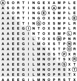
The first pass has no effect in this example, because there is no element in the array smaller than the A at the left. On the second pass, the other A is the smallest remaining element, so it is exchanged with the S in the second position. Then, the E near the middle is exchanged with the O in the third position on the third pass; then, the other E is exchanged with the R in the fourth position on the fourth pass; and so forth.
Figure 6.2 Selection sort example
Program 6.2 is an implementation of selection sort that adheres to our conventions. The inner loop is just a comparison to test a current element against the smallest element found so far (plus the code necessary to increment the index of the current element and to check that it does not exceed the array bounds); it could hardly be simpler. The work of moving the items around falls outside the inner loop: each exchange puts an element into its final position, so the number of exchanges is N – 1 (no exchange is needed for the final element). Thus the running time is dominated by the number of comparisons. In Section 6.5, we show this number to be proportional to N2, and examine more closely how to predict the total running time and how to compare selection sort with other elementary sorts.
A disadvantage of selection sort is that its running time depends only slightly on the amount of order already in the file. The process of finding the minimum element on one pass through the file does not seem to give much information about where the minimum might be on the next pass through the file. For example, the user of the sort might be surprised to realize that it takes about as long to run selection sort for a file that is already in order, or for a file with all keys equal, as it does for a randomly ordered file! As we shall see, other methods are better able to take advantage of order in the input file.
Despite its simplicity and evident brute-force approach, selection sort outperforms more sophisticated methods in one important application: it is the method of choice for sorting files with huge items and small keys. For such applications, the cost of moving the data dominates the cost of making comparisons, and no algorithm can sort a file with substantially less data movement than selection sort (see Property 6.5 in Section 6.5).
Exercises
![]() 6.11 Show, in the style of Figure 6.2, how selection sort sorts the sample file E A S Y Q U E S T I O N.
6.11 Show, in the style of Figure 6.2, how selection sort sorts the sample file E A S Y Q U E S T I O N.
6.12 What is the maximum number of exchanges involving any particular element during selection sort? What is the average number of exchanges involving an element?
6.13 Give an example of a file of N elements that maximizes the number of times the test less(a[j], a[min]) fails (and, therefore, min gets updated) during the operation of selection sort.
![]() 6.14 Is selection sort stable?
6.14 Is selection sort stable?
6.3 Insertion Sort
The method that people often use to sort bridge hands is to consider the elements one at a time, inserting each into its proper place among those already considered (keeping them sorted). In a computer implementation, we need to make space for the element being inserted by moving larger elements one position to the right, and then inserting the element into the vacated position. The sort function in Program 6.1 is an implementation of this method, which is called insertion sort.
As in selection sort, the elements to the left of the current index are in sorted order during the sort, but they are not in their final position, as they may have to be moved to make room for smaller elements encountered later. The array is, however, fully sorted when the index reaches the right end. Figure 6.3 shows the method in operation on a sample file.
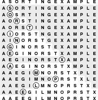
During the first pass of insertion sort, the S in the second position is larger than the A, so it does not have to be moved. On the second pass, when the O in the third position is encountered, it is exchanged with the S to put A O S in sorted order, and so forth. Un-shaded elements that are not circled are those that were moved one position to the right.
Figure 6.3 Insertion sort example
The implementation of insertion sort in Program 6.1 is straightforward, but inefficient. We shall now consider three ways to improve it, to illustrate a recurrent theme throughout many of our implementations: We want code to be succinct, clear, and efficient, but these goals sometimes conflict, so we must often strike a balance. We do so by developing a natural implementation, then seeking to improve it by a sequence of transformations, checking the effectiveness (and correctness) of each transformation.
First, we can stop doing compexch operations when we encounter a key that is not larger than the key in the item being inserted, because the subarray to the left is sorted. Specifically, we can break out of the inner for loop in sort in Program 6.1 when the condition less(a[j-1], a[j]) is true. This modification changes the implementation into an adaptive sort, and speeds up the program by about a factor of 2 for randomly ordered keys (see Property 6.2).
With the improvement described in the previous paragraph, we have two conditions that terminate the inner loop—we could recode it as a while loop to reflect that fact explicitly. A more subtle improvement of the implementation follows from noting that the test j>l is usually extraneous: indeed, it succeeds only when the element inserted is the smallest seen so far and reaches the beginning of the array. A commonly used alternative is to keep the keys to be sorted in a[1] to a[N], and to put a sentinel key in a[0], making it at least as small as the smallest key in the array. Then, the test whether a smaller key has been encountered simultaneously tests both conditions of interest, making the inner loop smaller and the program faster.
Sentinels are sometimes inconvenient to use: perhaps the smallest possible key is not easily defined, or perhaps the calling routine has no room to include an extra key. Program 6.3 illustrates one way around these two problems for insertion sort: We make an explicit first pass over the array that puts the item with the smallest key in the first position. Then, we sort the rest of the array, with that first and smallest item now serving as sentinel. We generally shall avoid sentinels in our code, because it is often easier to understand code with explicit tests, but we shall note situations where sentinels might be useful in making programs both simpler and more efficient.
The third improvement that we shall consider also involves removing extraneous instructions from the inner loop. It follows from noting that successive exchanges involving the same element are inefficient. If there are two or more exchanges, we have
t = a[j]; a[j] = a[j-1]; a[j-1] = t;
followed by
t = a[j-1]; a[j-1] = a[j-2]; a[j-2] = t;
and so forth. The value of t does not change between these two sequences, and we waste time storing it, then reloading it for the next exchange. Program 6.3 moves larger elements one position to the right instead of using exchanges, and thus avoids wasting time in this way.
Program 6.3 is an implementation of insertion sort that is more efficient than the one given in Program 6.1 (in Section 6.5, we shall see that it is nearly twice as fast). In this book, we are interested both in elegant and efficient algorithms and in elegant and efficient implementations of them. In this case, the underlying algorithms do differ slightly—we should properly refer to the sort function in Program 6.1 as a nonadaptive insertion sort. A good understanding of the properties of an algorithm is the best guide to developing an implementation that can be used effectively in an application.
Unlike that of selection sort, the running time of insertion sort primarily depends on the initial order of the keys in the input. For example, if the file is large and the keys are already in order (or even are nearly in order), then insertion sort is quick and selection sort is slow. We compare the algorithms in more detail in Section 6.5.
Exercises
![]() 6.15 Show, in the style of Figure 6.3, how insertion sort sorts the sample file E A S Y Q U E S T I O N.
6.15 Show, in the style of Figure 6.3, how insertion sort sorts the sample file E A S Y Q U E S T I O N.
6.16 Give an implementation of insertion sort with the inner loop coded as a while loop that terminates on one of two conditions, as described in the text.
6.17 For each of the conditions in the while loop in Exercise 6.16, describe a file of N elements where that condition is always false when the loop terminates.
![]() 6.18 Is insertion sort stable?
6.18 Is insertion sort stable?
6.19 Give a nonadaptive implementation of selection sort based on finding the minimum element with code like the first for loop in Program 6.3.
6.4 Bubble Sort
The first sort that many people learn, because it is so simple, is bubble sort: Keep passing through the file, exchanging adjacent elements that are out of order, continuing until the file is sorted. Bubble sort’s prime virtue is that it is easy to implement, but whether it is actually easier to implement than insertion or selection sort is arguable. Bubble sort generally will be slower than the other two methods, but we consider it briefly for the sake of completeness.
Suppose that we always move from right to left through the file. Whenever the minimum element is encountered during the first pass, we exchange it with each of the elements to its left, eventually putting it into position at the left end of the array. Then on the second pass, the second smallest element will be put into position, and so forth. Thus, N passes suffice, and bubble sort operates as a type of selection sort, although it does more work to get each element into position. Program 6.4 is an implementation, and Figure 6.4 shows an example of the algorithm in operation.
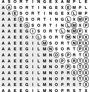
Small keys percolate over to the left in bubble sort. As the sort moves from right to left, each key is exchanged with the one on its left until a smaller one is encountered. On the first pass, the E is exchanged with the L, the P, and the M before stopping at the A on the right; then the A moves to the beginning of the file, stopping at the other A, which is already in position. The ith smallest key reaches its final position after the ith pass, just as in selection sort, but other keys are moved closer to their final position, as well.
Figure 6.4 Bubble sort example
We can speed up Program 6.4 by carefully implementing the inner loop, in much the same way as we did in Section 6.3 for insertion sort (see Exercise 6.25). Indeed, comparing the code, Program 6.4 appears to be virtually identical to the nonadaptive insertion sort in Program 6.1. The difference between the two is that the inner for loop moves through the left (sorted) part of the array for insertion sort and through the right (not necessarily sorted) part of the array for bubble sort.
Program 6.4 uses only compexch instructions and is therefore nonadaptive, but we can improve it to run more efficiently when the file is nearly in order by testing whether no exchanges at all are performed on one of the passes (and therefore the file is in sorted order, so we can break out of the outer loop). Adding this improvement will make bubble sort faster on some types of files, but it is generally not as effective as is changing insertion sort to break out of the inner loop, as discussed in detail in Section 6.5.
Exercises
![]() 6.20 Show, in the style of Figure 6.4, how bubble sort sorts the sample file E A S Y Q U E S T I O N.
6.20 Show, in the style of Figure 6.4, how bubble sort sorts the sample file E A S Y Q U E S T I O N.
6.21 Give an example of a file for which the number of exchanges done by bubble sort is maximized.
6.23 Explain how bubble sort is preferable to the nonadaptive version of selection sort described in Exercise 6.19.
![]() 6.24 Do experiments to determine how many passes are saved, for random files of N elements, when you add to bubble sort a test to terminate when the file is sorted.
6.24 Do experiments to determine how many passes are saved, for random files of N elements, when you add to bubble sort a test to terminate when the file is sorted.
6.25 Develop an efficient implementation of bubble sort, with as few instructions as possible in the inner loop. Make sure that your “improvements” do not slow down the program!
6.5 Performance Characteristics of Elementary Sorts
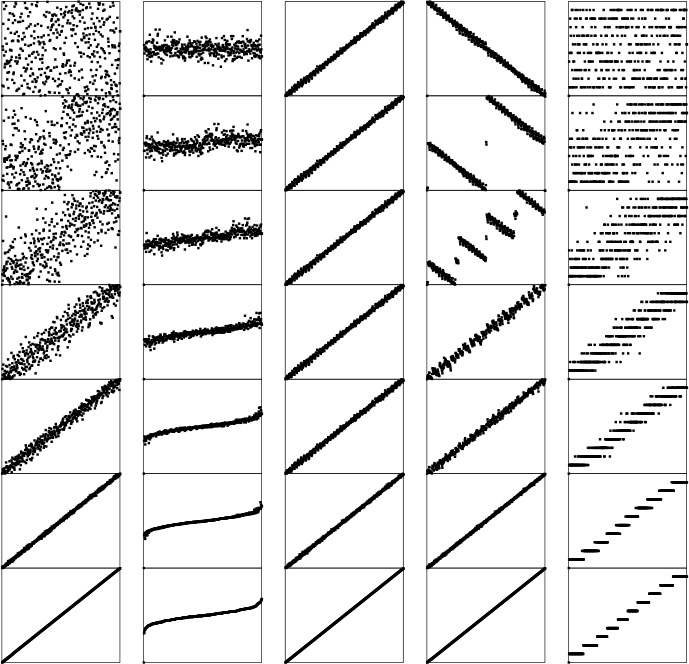
Selection sort, insertion sort, and bubble sort are all quadratic-time algorithms both in the worst and in the average case, and none requires extra memory. Their running times thus differ by only a constant factor, but they operate quite differently, as illustrated in Figures 6.5 through 6.7.
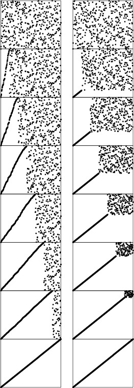
These snapshots of insertion sort (left) and selection sort (right) in action on a random permutation illustrate how each method progresses through the sort. We represent an array being sorted by plotting i vs. a[i] for each i. Before the sort, the plot is uniformly random; after the sort, it is a diagonal line from bottom left to top right. Insertion sort never looks ahead of its current position in the array; selection sort never looks back.
Figure 6.5 Dynamic characteristics of insertion and selection sorts
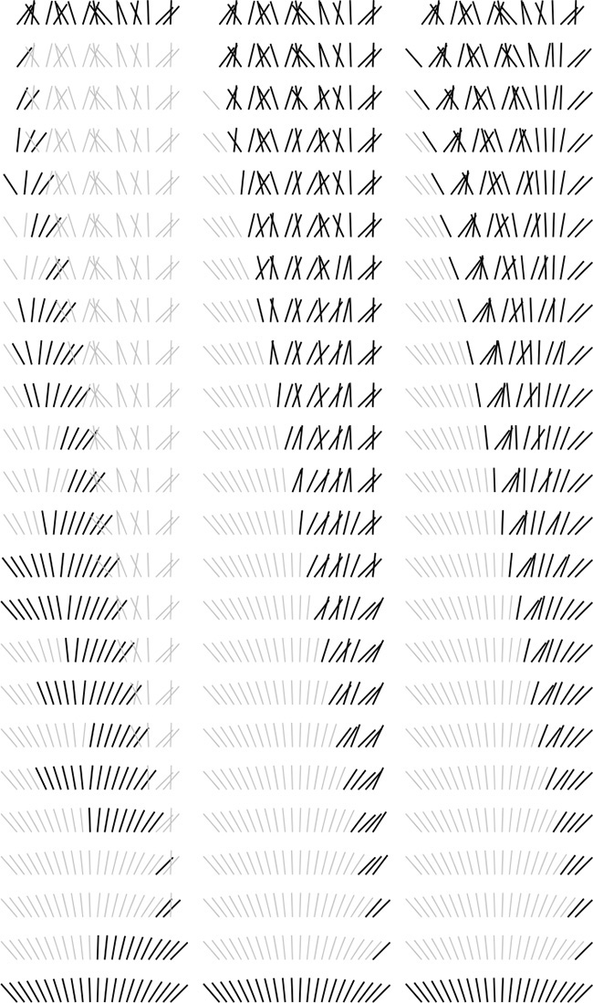
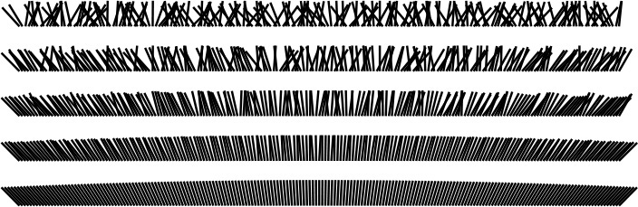
This diagram highlights the differences in the way that insertion sort, selection sort, and bubble sort bring a file into order. The file to be sorted is represented by lines that are to be sorted according to their angles. Black lines correspond to the items accessed during each pass of the sort; gray lines correspond to items not touched. For insertion sort (left), the element to be inserted goes about halfway back through the sorted part of the file on each pass. Selection sort (center) and bubble sort (right) both go through the entire unsorted part of the array to find the next smallest element there for each pass; the difference between the methods is that bubble sort exchanges any adjacent out-of-order elements that it encounters, whereas selection sort just exchanges the minimum into position. The effect of this difference is that the unsorted part of the array becomes more nearly sorted as bubble sort progresses.
Figure 6.6 Comparisons and exchanges in elementary sorts
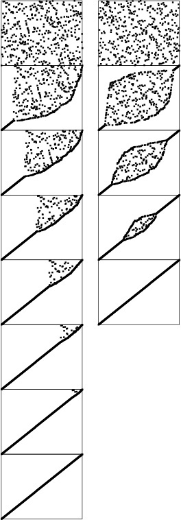
Standard bubble sort (left) operates in a manner similar to selection sort in that each pass brings one element into position, but it also brings some order into other parts of the array, in an asymmetric manner. Changing the scan through the array to alternate between beginning to end and end to beginning gives a version of bubble sort called shaker sort (right), which finishes more quickly (see Exercise 6.30).
Figure 6.7 Dynamic characteristics of two bubble sorts
Generally, the running time of a sorting algorithm is proportional to the number of comparisons that the algorithm uses, to the number of times that items are moved or exchanged, or to both. For random input, comparing the methods involves studying constant-factor differences in the numbers of comparisons and exchanges and constant-factor differences in the lengths of the inner loops. For input with special characteristics, the running times of the methods may differ by more than a constant factor. In this section, we look closely at the analytic results in support of this conclusion.
Property 6.1 Selection sort uses about N2/2 comparisons and N exchanges.
We can verify this property easily by examining the sample run in Figure 6.2, which is an N-by-N table in which unshaded letters correspond to comparisons. About one-half of the elements in the table are unshaded—those above the diagonal. The N – 1 (not the final one) elements on the diagonal each correspond to an exchange. More precisely, examination of the code reveals that, for each i from 1 to N – 1, there is one exchange and N – i comparisons, so there is a total of N – 1 exchanges and (N – 1) + (N – 2)+ ···+2+1 = N(N – 1)/2 comparisons. These observations hold no matter what the input data are; the only part of selection sort that does depend on the input is the number of times that min is updated. In the worst case, this quantity could also be quadratic; in the average case, however, it is just O(N log N) (see reference section), so we can expect the running time of selection sort to be insensitive to the input. ![]()
Property 6.2 Insertion sort uses about N2/4 comparisons and N2/4 half-exchanges (moves) on the average, and twice that many at worst.
As implemented in Program 6.3, the number of comparisons and of moves is the same. Just as for Property 6.1, this quantity is easy to visualize in the N-by-N diagram in Figure 6.3 that gives the details of the operation of the algorithm. Here, the elements below the diagonal are counted—all of them, in the worst case. For random input, we expect each element to go about halfway back, on the average, so one-half of the elements below the diagonal should be counted. ![]()
Property 6.3 Bubble sort uses about N2/2 comparisons and N2/2 exchanges on the average and in the worst case.
The ith bubble sort pass requires N – i compare–exchange operations, so the proof goes as for selection sort. When the algorithm is modified to terminate when it discovers that the file is sorted, the running time depends on the input. Just one pass is required if the file is already in order, but the ith pass requires N – i comparisons and exchanges if the file is in reverse order. The average-case performance is not significantly better than the worst case, as stated, although the analysis that demonstrates this fact is complicated (see reference section). ![]()
Although the concept of a partially sorted file is necessarily rather imprecise, insertion sort and bubble sort work well for certain types of nonrandom files that often arise in practice. General-purpose sorts are commonly misused for such applications. For example, consider the operation of insertion sort on a file that is already sorted. Each element is immediately determined to be in its proper place in the file, and the total running time is linear. The same is true for bubble sort, but selection sort is still quadratic.
Definition 6.2 An inversion is a pair of keys that are out of order in the file.
To count the number of inversions in a file, we can add up, for each element, the number of elements to its left that are greater (we refer to this quantity as the number of inversions corresponding to the element). But this count is precisely the distance that the elements have to move when inserted into the file during insertion sort. A file that has some order will have fewer inversions than will one that is arbitrarily scrambled.
In one type of partially sorted file, each item is close to its final position in the file. For example, some people sort their hand in a card game by first organizing the cards by suit, to put their cards close to their final position, then considering the cards one by one. We shall be considering a number of sorting methods that work in much the same way—they bring elements close to final positions in early stages to produce a partially sorted file with every element not far from where it ultimately must go. Insertion sort and bubble sort (but not selection sort) are efficient methods for sorting such files.
Property 6.4 Insertion sort and bubble sort use a linear number of comparisons and exchanges for files with at most a constant number of inversions corresponding to each element.
As just mentioned, the running time of insertion sort is directly proportional to the number of inversions in the file. For bubble sort (here, we are referring to Program 6.4, modified to terminate when the file is sorted), the proof is more subtle (see Exercise 6.29). Each bubble sort pass reduces the number of smaller elements to the right of any element by precisely 1 (unless the number was already 0), so bubble sort uses at most a constant number of passes for the types of files under consideration, and therefore does at most a linear number of comparisons and exchanges. ![]()
In another type of partially sorted file, we perhaps have appended a few elements to a sorted file or have edited a few elements in a sorted file to change their keys. This kind of file is prevalent in sorting applications. Insertion sort is an efficient method for such files; bubble sort and selection sort are not.
Property 6.5 Insertion sort uses a linear number of comparisons and exchanges for files with at most a constant number of elements having more than a constant number of corresponding inversions.
The running time of insertion sort depends on the total number of inversions in the file, and does not depend on the way in which the inversions are distributed. ![]()
To draw conclusions about running time from Properties 6.1 through 6.5, we need to analyze the relative cost of comparisons and exchanges, a factor that in turn depends on the size of the items and keys (see Table 6.1). For example, if the items are one-word keys, then an exchange (four array accesses) should be about twice as expensive as a comparison. In such a situation, the running times of selection and insertion sort are roughly comparable, but bubble sort is slower. But if the items are large in comparison to the keys, then selection sort will be best.
Insertion sort and selection sort are about twice as fast as bubble sort for small files, but running times grow quadratically (when the file size grows by a factor of 2, the running time grows by a factor of 4). None of the methods are useful for large randomly ordered files—for example, the numbers corresponding to those in this table are less than 2 for the shellsort algorithm in Section 6.6. When comparisons are expensive—for example, when the keys are strings—then insertion sort is much faster than the other two because it uses many fewer comparisons. Not included here is the case where exchanges are expensive; then selection sort is best.
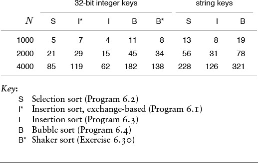
Table 6.1 Empirical study of elementary sorting algorithms
Property 6.6 Selection sort runs in linear time for files with large items and small keys.
Let M be the ratio of the size of the item to the size of the key. Then we can assume the cost of a comparison to be 1 time unit and the cost of an exchange to be M time units. Selection sort takes about N2/2 time units for comparisons and about NM time units for exchanges. If M is larger than a constant multiple of N, then the NM term dominates the N2 term, so the running time is proportional to NM, which is proportional to the amount of time that would be required to move all the data. ![]()
For example, if we have to sort 1000 items that consist of 1-word keys and 1000 words of data each, and we actually have to rearrange the items, then we cannot do better than selection sort, since the running time will be dominated by the cost of moving all 1 million words of data. In Section 6.8, we shall see alternatives to rearranging the data.
Exercises
![]() 6.26 Which of the three elementary methods (selection sort, insertion sort, or bubble sort) runs fastest for a file with all keys identical?
6.26 Which of the three elementary methods (selection sort, insertion sort, or bubble sort) runs fastest for a file with all keys identical?
6.27 Which of the three elementary methods runs fastest for a file in reverse order?
6.28 Give an example of a file of 10 elements (use the keys A through J) for which bubble sort uses fewer comparisons than insertion sort, or prove that no such file exists.
![]() 6.29 Show that each bubble sort pass reduces by precisely 1 the number of elements to the left of each element that are greater (unless that number was already 0).
6.29 Show that each bubble sort pass reduces by precisely 1 the number of elements to the left of each element that are greater (unless that number was already 0).
6.30 Implement a version of bubble sort that alternates left-to-right and right-to-left passes through the data. This (faster but more complicated) algorithm is called shaker sort (see Figure 6.7).
![]() 6.31 Show that Property 6.5 does not hold for shaker sort (see Exercise 6.30).
6.31 Show that Property 6.5 does not hold for shaker sort (see Exercise 6.30).
![]() 6.32 Implement selection sort in PostScript (see Section 4.3), and use your implementation to draw figures like Figures 6.5 through 6.7. You may try a recursive implementation, or read the manual to learn about loops and arrays in PostScript.
6.32 Implement selection sort in PostScript (see Section 4.3), and use your implementation to draw figures like Figures 6.5 through 6.7. You may try a recursive implementation, or read the manual to learn about loops and arrays in PostScript.
6.6 Shellsort
Insertion sort is slow because the only exchanges it does involve adjacent items, so items can move through the array only one place at a time. For example, if the item with the smallest key happens to be at the end of the array, N steps are needed to get it where it belongs. Shellsort is a simple extension of insertion sort that gains speed by allowing exchanges of elements that are far apart.
The idea is to rearrange the file to give it the property that taking every hth element (starting anywhere) yields a sorted file. Such a file is said to be h-sorted. Put another way, an h-sorted file is h independent sorted files, interleaved together. By h-sorting for some large values of h, we can move elements in the array long distances and thus make it easier to h-sort for smaller values of h. Using such a procedure for any sequence of values of h that ends in 1 will produce a sorted file: that is the essence of shellsort.
One way to implement shellsort would be, for each h, to use insertion sort independently on each of the h subfiles. Despite the apparent simplicity of this process, we can use an even simpler approach, precisely because the subfiles are independent. When h-sorting the file, we simply insert it among the previous elements in its h-subfile by moving larger elements to the right (see Figure 6.8). We accomplish this task by using the insertion-sort code, but modified to increment or decrement by h instead of 1 when moving through the file. This observation reduces the shellsort implementation to nothing more than an insertion-sort–like pass through the file for each increment, as in Program 6.5. The operation of this program is illustrated in Figure 6.9.
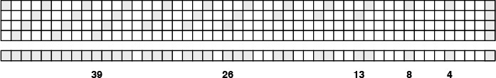
The top part of this diagram shows the process of 4-sorting a file of 15 elements by first insertion sorting the subfile at positions 0, 4, 8, 12, then insertion sorting the subfile at positions 1, 5, 9, 13, then insertion sorting the subfile at positions 2, 6, 10, 14, then insertion sorting the subfile at positions 3, 7, 11. But the four subfiles are independent, so we can achieve the same result by inserting each element into position into its subfile, going back four at a time (bottom). Taking the first row in each section of the top diagram, then the second row in each section, and so forth, gives the bottom diagram.
Figure 6.8 Interleaving 4-sorts

Sorting a file by 13-sorting (top), then 4-sorting (center), then 1-sorting (bottom) does not involve many comparisons (as indicated by the unshaded elements). The final pass is just insertion sort, but no element has to move far because of the order in the file due to the first two passes.
Figure 6.9 Shellsort example
How do we decide what increment sequence to use? In general, this question is a difficult one to answer. Properties of many different increment sequences have been studied in the literature, and some have been found that work well in practice, but no provably best sequence has been found. In practice, we generally use sequences that decrease roughly geometrically, so the number of increments is logarithmic in the size of the file. For example, if each increment is about one-half of the previous, then we need only about 20 increments to sort a file of 1 million elements; if the ratio is about one-quarter, then 10 increments will suffice. Using as few increments as possible is an important consideration that is easy to respect—we also need to consider arithmetical interactions among the increments such as the size of their common divisors and other properties.
The practical effect of finding a good increment sequence is limited to perhaps a 25% speedup, but the problem presents an intriguing puzzle that provides a good example of the inherent complexity in an apparently simple algorithm.
The increment sequence 1 4 13 40 121 364 1093 3280 9841 ... that is used in Program 6.5, with a ratio between increments of about one-third, was recommended by Knuth in 1969 (see reference section). It is easy to compute (start with 1, generate the next increment by multiplying by 3 and adding 1) and leads to a relatively efficient sort, even for moderately large files, as illustrated in Figure 6.10.
The effect of each of the passes in Shellsort is to bring the file as a whole closer to sorted order. The file is first 40-sorted, then 13-sorted, then 4-sorted, then 1-sorted. Each pass brings the file closer to sorted order.
Figure 6.10 Shellsorting a random permutation
Many other increment sequences lead to a more efficient sort but it is difficult to beat the sequence in Program 6.5 by more than 20% even for relatively large N. One increment sequence that does so is 1 8 23 77 281 1073 4193 16577 ..., the sequence 4i+1 + 3 · 2i + 1 for i > 0, which has provably faster worst-case behavior (see Property 6.10). Figure 6.12 shows that this sequence and Knuth’s sequence—and many other sequences—have similar dynamic characteristics for large files. The possibility that even better increment sequences exist is still real. A few ideas on improved increment sequences are explored in the exercises.
On the other hand, there are some bad increment sequences: for example 1 2 4 8 16 32 64 128 256 512 1024 2048 ... (the original sequence suggested by Shell when he proposed the algorithm in 1959 (see reference section)) is likely to lead to bad performance because elements in odd positions are not compared against elements in even positions until the final pass. The effect is noticeable for random files, and is catastrophic in the worst case: The method degenerates to require quadratic running time if, for example, the half of the elements with the smallest values are in even positions and the half of the elements with the largest values are in the odd positions (See Exercise 6.36.)
Program 6.5 computes the next increment by dividing the current one by 3, after initializing to ensure that the same sequence is always used. Another option is just to start with h = N/3 or with some other function of N. It is best to avoid such strategies, because bad sequences of the type described in the previous paragraph are likely to turn up for some values of N.
Our description of the efficiency of shellsort is necessarily imprecise, because no one has been able to analyze the algorithm. This gap in our knowledge makes it difficult not only to evaluate different increment sequences, but also to compare shellsort with other methods analytically. Not even the functional form of the running time for shellsort is known (furthermore, the form depends on the increment sequence). Knuth found that the functional forms N(log N)2 and N1.25 both fit the data reasonably well, and later research suggests that a more complicated function of the form ![]() is involved for some sequences.
is involved for some sequences.
We conclude this section by digressing into a discussion of several facts about the analysis of shellsort that are known. Our primary purpose in doing so is to illustrate that even algorithms that are apparently simple can have complex properties, and that the analysis of algorithms is not just of practical importance but also can be intellectually challenging. Readers intrigued by the idea of finding a new and improved shellsort increment sequence may find the information that follows useful; other readers may wish to skip to Section 6.7.
Property 6.7 The result of h-sorting a file that is k-ordered is a file that is both h- and k-ordered.
This fact seems obvious, but is tricky to prove (see Exercise 6.47). ![]()
Property 6.8 Shellsort does less than N(h – 1)(k – 1)/g comparisons to g-sort a file that is h- and k-ordered, provided that h and k are relatively prime.
The basis for this fact is illustrated in Figure 6.11. No element farther than (h – 1)(k – 1) positions to the left of any given element x can be greater than x, if h and k are relatively prime (see Exercise 6.43). When g-sorting, we examine at most one out of every g of those elements. ![]()
The bottom row depicts an array, with shaded boxes depicting those items that must be smaller than or equal to the item at the far right, if the array is both 4- and 13-ordered. The four rows at top depict the origin of the pattern. If the item at right is at array position i, then 4-ordering means that items at array positions i–4, i–8, i–12, ... are smaller or equal (top); 13-ordering means that the item at i – 13, and, therefore, because of 4-ordering, the items at i – 17, i – 21, i – 25, ... are smaller or equal (second from top); also, the item at i – 26, and, therefore, because of 4-ordering, the items at i–30, i–34, i–38, ... are smaller or equal (third from top); and so forth. The white squares remaining are those that could be larger than the item at left; there are at most 18 such items (and the one that is farthest away is at i – 36). Thus, at most 18N comparisons are required for an insertion sort of a 13-ordered and 4-ordered file of size N.
Figure 6.11 A 4- and 13- ordered file.
Property 6.9 Shellsort does less than O(N3/2) comparisons for the increments 1 4 13 40 121 364 1093 3280 9841 ... .
For large increments, there are h subfiles of size about N/h, for a worst-case cost about N2/h. For small increments, Property 6.8 implies that the cost is about Nh. The result follows if we use the better of these bounds for each increment. It holds for any relatively prime sequence that grows exponentially. ![]()
Property 6.10 Shellsort does less than O(N4/3) comparisons for the increments 1 8 23 77 281 1073 4193 16577 ... .
The proof of this property is along the lines of the proof of Property 6.9. The property analogous to Property 6.8 implies that the cost for small increments is about Nh1/2. Proof of this property requires number theory that is beyond the scope of this book (see reference section). ![]()
The increment sequences that we have discussed to this point are effective because successive elements are relatively prime. Another family of increment sequences is effective precisely because successive elements are not relatively prime.
In particular, the proof of Property 6.8 implies that, in a file that is 2-ordered and 3-ordered, each element moves at most one position during the final insertion sort. That is, such a file can be sorted with one bubble-sort pass (the extra loop in insertion sort is not needed). Now, if a file is 4-ordered and 6-ordered, then it also follows that each element moves at most one position when we are 2-sorting it (because each subfile is 2-ordered and 3-ordered); and if a file is 6-ordered and 9-ordered, each element moves at most one position when we are 3-sorting it. Continuing this line of reasoning, we are led to the following idea, which was developed by Pratt in 1971 (see reference section).
Property 6.11 Shellsort does less than O(N(log N)2) comparisons for the increments 1 2 3 4 6 9 8 12 18 27 16 24 36 54 81 ... .
Consider the following triangle of increments, where each number in the triangle is two times the number above and to the right of it and also three times the number above and to the left of it.

If we use these numbers from bottom to top and right to left as a shellsort increment sequence, then every increment x after the bottom row is preceded by 2x and 3x, so every subfile is 2-ordered and 3-ordered, and no element moves more than one position during the entire sort! The number of increments in the triangle that are less than N is certainly less than (log2 N)2. ![]()
Pratt’s increments tend not to work as well as the others in practice, because there are too many of them. We can use the same principle to build an increment sequence from any two relatively prime numbers h and k. Such sequences do well in practice because the worst-case bounds corresponding to Property 6.11 overestimate the cost for random files.
The problem of designing good increment sequences for shellsort provides an excellent example of the complex behavior of a simple algorithm. We certainly will not be able to focus at this level of detail on all the algorithms that we encounter (not only do we not have the space, but also, as we did with shellsort, we might encounter mathematical analysis beyond the scope of this book, or even open research problems). However, many of the algorithms in this book are the product of extensive analytic and empirical studies by many researchers over the past several decades, and we can benefit from this work. This research illustrates that the quest for improved performance can be both intellectually challenging and practically rewarding, even for simple algorithms. Table 6.2 gives empirical results that show that several approaches to designing increment sequences work well in practice; the relatively short sequence 1 8 23 77 281 1073 4193 16577 ... is among the simplest to use in a shellsort implementation.
Shellsort is many times faster than the other elementary methods even when the increments are powers of 2, but some increment sequences can speed it up by another factor of 5 or more. The three best sequences in this table are totally different in design. Shellsort is a practical method even for large files, particularly by contrast with selection sort, insertion sort, and bubble sort (see Table 6.1).

Table 6.2 Empirical study of shellsort increment sequences
Figure 6.13 shows that shellsort performs reasonably well on a variety of kinds of files, rather than just on random ones. Indeed, constructing a file for which shellsort runs slowly for a given increment sequence is a challenging exercise (see Exercise 6.42). As we have mentioned, there are some bad increment sequences for which shellsort may require a quadratic number of comparisons in the worst case (see Exercise 6.36), but much lower bounds have been shown to hold for a wide variety of sequences.
In this representation of shellsort in operation, it appears as though a rubber band, anchored at the corners, is pulling the points toward the diagonal. Two increment sequences are depicted: 121 40 13 4 1 (left) and 209 109 41 19 5 1 (right). The second requires one more pass than the first, but is faster because each pass is more efficient.
Figure 6.12 Dynamic characteristics of shellsort (two different increment sequences)
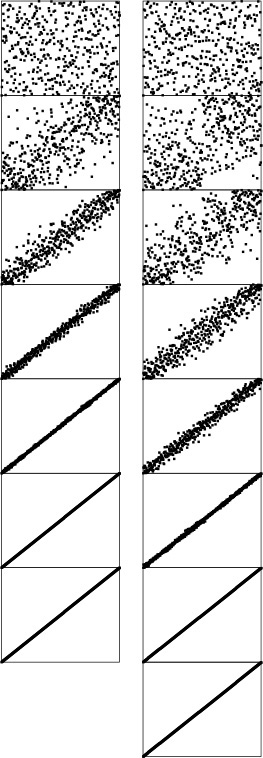
These diagrams show shellsort, with the increments 209 109 41 19 5 1, in operation on files that are random, Gaussian, nearly ordered, nearly reverse-ordered, and randomly ordered with 10 distinct key values (left to right, on the top). The running time for each pass depends on how well ordered the file is when the pass begins. After a few passes, these files are similarly ordered; thus, the running time is not particularly sensitive to the input.
Figure 6.13 Dynamic characteristics of shellsort for various types of files
Shellsort is the method of choice for many sorting applications because it has acceptable running time even for moderately large files and requires a small amount of code that is easy to get working. In the next few chapters, we shall see methods that are more efficient, but they are perhaps only twice as fast (if that much) except for large N, and they are significantly more complicated. In short, if you need a quick solution to a sorting problem, and do not want to bother with interfacing to a system sort, you can use shellsort, then determine sometime later whether the extra work required to replace it with a more sophisticated method will be worthwhile.
6.34 Show how to implement a shellsort with the increments 1 8 23 77 281 1073 4193 16577 ..., with direct calculations to get successive increments in a manner similar to the code given for Knuth’s increments.
![]() 6.35 Give diagrams corresponding to Figures 6.8 and 6.9 for the keys E A S Y Q U E S T I O N.
6.35 Give diagrams corresponding to Figures 6.8 and 6.9 for the keys E A S Y Q U E S T I O N.
6.36 Find the running time when you use shellsort with the increments 1 2 4 8 16 32 64 128 256 512 1024 2048 ... to sort a file consisting of the integers 1, 2, ..., N in the odd positions and N + 1, N + 2, ..., 2N in the even positions.
6.37 Write a driver program to compare increment sequences for shellsort. Read the sequences from standard input, one per line, then use them all to sort 10 random files of size N for N = 100, 1000, and 10000. Count comparisons, or measure actual running times.
![]() 6.38 Run experiments to determine whether adding or deleting an increment can improve the increment sequence 1 8 23 77 281 1073 4193 16577 ... for N = 10000.
6.38 Run experiments to determine whether adding or deleting an increment can improve the increment sequence 1 8 23 77 281 1073 4193 16577 ... for N = 10000.
![]() 6.39 Run experiments to determine the value of x that leads to the lowest running time for random files when the 13 is replaced by x in the increment sequence 1 4 13 40 121 364 1093 3280 9841 ... used for N = 10000.
6.39 Run experiments to determine the value of x that leads to the lowest running time for random files when the 13 is replaced by x in the increment sequence 1 4 13 40 121 364 1093 3280 9841 ... used for N = 10000.
6.40 Run experiments to determine the value of α that leads to the lowest running time for random files for the increment sequence 1, ![]() α
α![]() ,
, ![]() α2
α2![]() ,
, ![]() α3
α3![]() ,
, ![]() α4
α4![]() , ...; for N = 10000.
, ...; for N = 10000.
![]() 6.41 Find the three-increment sequence that uses as small a number of comparisons as you can find for random files of 1000 elements.
6.41 Find the three-increment sequence that uses as small a number of comparisons as you can find for random files of 1000 elements.
![]() 6.42 Construct a file of 100 elements for which shellsort, with the increments 1 8 23 77, uses as large a number of comparisons as you can find.
6.42 Construct a file of 100 elements for which shellsort, with the increments 1 8 23 77, uses as large a number of comparisons as you can find.
![]() 6.43 Prove that any number greater than or equal to (h – 1)(k – 1) can be expressed as a linear combination (with nonnegative coefficients) of h and k, if h and k are relatively prime. Hint: Show that, if any two of the first h – 1 multiples of k have the same remainder when divided by h, then h and k must have a common factor.
6.43 Prove that any number greater than or equal to (h – 1)(k – 1) can be expressed as a linear combination (with nonnegative coefficients) of h and k, if h and k are relatively prime. Hint: Show that, if any two of the first h – 1 multiples of k have the same remainder when divided by h, then h and k must have a common factor.
6.44 Run experiments to determine the values of h and k that lead to the lowest running times for random files when a Pratt-like sequence based on h and k is used for sorting 10000 elements.
6.45 The increment sequence 1 5 19 41 109 209 505 929 2161 3905 ... is based on merging the sequences 9·4i – 9·2i + 1 and 4i – 3·2i + 1 for i > 0. Compare the results of using these sequences individually and using the merged result, for sorting 10000 elements.
6.46 We derive the increment sequence 1 3 7 21 48 112 336 861 1968 4592 13776 ... by starting with a base sequence of relatively prime numbers, say 1 3 7 16 41 101, then building a triangle, as in Pratt’s sequence, this time generating the ith row in the triangle by multiplying the first element in the i – 1st row by the ith element in the base sequence; and multiplying every element in the i – 1st row by the i + 1st element in the base sequence. Run experiments to find a base sequence that improves on the one given for sorting 10000 elements.
![]() 6.47 Complete the proofs of Properties 6.7 and 6.8.
6.47 Complete the proofs of Properties 6.7 and 6.8.
![]() 6.48 Implement a shellsort that is based on the shaker sort algorithm of Exercise 6.30, and compare with the standard algorithm. Note: Your increment sequences should be substantially different from those for the standard algorithm.
6.48 Implement a shellsort that is based on the shaker sort algorithm of Exercise 6.30, and compare with the standard algorithm. Note: Your increment sequences should be substantially different from those for the standard algorithm.
6.7 Sorting of Other Types of Data
Although it is reasonable to learn most algorithms by thinking of them as simply sorting arrays of numbers into numerical order or characters into alphabetical order, it is also worthwhile to recognize that the algorithms are largely independent of the type of items being sorted, and that is not difficult to move to a more general setting. We have talked in detail about breaking our programs into independent modules to implement data types, and abstract data types (see Chapters 3 and 4); in this section, we consider ways in which we can apply the concepts discussed there to make our sorting implementations useful for various types of data.
Specifically, we consider implementations, interfaces, and client programs for:
• Items, or generic objects to be sorted
• Arrays of items
The item data type provides us with a way to use our sort code for any type of data for which certain basic operations are defined. The approach is effective both for simple data types and for abstract data types, and we shall consider numerous implementations. The array interface is less critical to our mission; we include it to give us an example of a mutiple-module program that uses multiple data types. We consider just one (straightforward) implementation of the array interface.
Program 6.6 is a client program with the same general functionality of the main program in Program 6.1, but with the code for manipulating arrays and items encapsulated in separate modules, which gives us, in particular, the ability to test various sort programs on various different types of data, by substituting various different modules, but without changing the client program at all. To complete the implementation, we need to define the array and item data type interfaces precisely, then provide implementations.
The interface in Program 6.7 defines examples of high-level operations that we might want to perform on arrays. We want to be able to initialize an array with key values, either randomly or from the standard input; we want to be able to sort the entries (of course!); and we want to be able to print out the contents. These are but a few examples; in a particular application, we might want to define various other operations. With this interface, we can substitute different implementations of the various operations without having to change the client program that uses the interface—main in Program 6.6, in this case. The various sort implementations that we are studying can serve as implementations for the sort function. Program 6.8 has simple implementations for the other functions. Again, we might wish to substitute other implementations, depending on the application. For example, we might use an implementation of show that prints out only part of the array when testing sorts on huge arrays.
In a similar manner, to work with particular types of items and keys, we define their types and declare all the relevant operations on them in an explicit interface, then provide implementations of the operations defined in the item interface. Program 6.9 is an example of such an interface for floating point keys. This code defines the operations that we have been using to compare keys and to exchange items, as well as functions to generate a random key, to read a key from standard input, and to print out the value of a key. Program 6.10 has implementations of these functions for this simple example. Some of the operations are defined as macros in the interface, which approach is generally more efficient; others are C code in the implementation, which approach is generally more flexible.
Programs 6.6 through 6.10 together with any of the sorting routines as is in Sections 6.2 through 6.6 provide a test of the sort for floating-point numbers. By providing similar interfaces and implementations for other types of data, we can put our sorts to use for a variety of data—such as long integers (see Exercise 6.49), complex numbers (see Exercise 6.50), or vectors (see Exercise 6.55)—without changing the sort code at all. For more complicated types of items, the interfaces and implementations have to be more complicated, but this implementation work is completely separated from the algorithm-design questions that we have been considering. We can use these same mechanisms with most of the sorting methods that we consider in this chapter and with those that we shall study in Chapters 7 through 9, as well. We consider in detail one important exception in Section 6.10—it leads to a whole family of important sorting algorithms that have to be packaged differently, the subject of Chapter 10.
The approach that we have discussed in this section is a middle road between Program 6.1 and an industrial-strength fully abstract set of implementations complete with error checking, memory management, and even more general capabilities. Packaging issues of this sort are of increasing importance in some modern programming and applications environments. We will necessarily leave some questions unanswered. Our primary purpose is to demonstrate, through the relatively simple mechanisms that we have examined, that the sorting implementations that we are studying are widely applicable.
Exercises
6.49 Write an interface and implementation for the generic item data type (similar to Programs 6.9 and 6.10) to support having the sorting methods sort long integers.
6.50 Write an interface and implementation for the generic item data type to support having the sorting methods sort complex numbers x + iy using the magnitude ![]() for the key. Note: Ignoring the square root is likely to improve efficiency.
for the key. Note: Ignoring the square root is likely to improve efficiency.
![]() 6.51 Write an interface that defines a first-class abstract data type for generic items (see Section 4.8), and provide an implementation where the items are floating point numbers. Test your program with Programs 6.3 and 6.6.
6.51 Write an interface that defines a first-class abstract data type for generic items (see Section 4.8), and provide an implementation where the items are floating point numbers. Test your program with Programs 6.3 and 6.6.
![]() 6.52 Add a function
6.52 Add a function check to the array data type in Programs 6.8 and 6.7, which tests whether or not the array is in sorted order.
![]() 6.53 Add a function
6.53 Add a function testinit to the array data type in Programs 6.8 and 6.7, which generates test data according to distributions similar to those illustrated in Figure 6.13. Provide an integer argument for the client to use to specify the distribution.
![]() 6.54 Change Programs 6.7 and 6.8 to implement an abstract data type. (Your implementation should allocate and maintain the array, as in our implementations for stacks and queues in Chapter 3.)
6.54 Change Programs 6.7 and 6.8 to implement an abstract data type. (Your implementation should allocate and maintain the array, as in our implementations for stacks and queues in Chapter 3.)
6.55 Write an interface and implementation for the generic item data type for use in having the sorting methods sort multidimensional vectors of d integers, putting the vectors in order by first component, those with equal first component in order by second component, those with equal first and second components in order by third component, and so forth.
6.8 Index and Pointer Sorting
The development of a string data type implementation similar to Programs 6.9 and 6.10 is of particular interest, because character strings are widely used as sort keys. Using the C library string-comparison function, we can change the first three lines in Program 6.9 to
typedef char *Item;
#define key(A) (A)
#define less(A, B) (strcmp(key(A), key(B)) < 0)
to convert it to an interface for strings.
The implementation is more challenging than Program 6.10 because, when working with strings in C, we must be aware of the allocation of memory for the strings. Program 6.11 uses the method that we examined in Chapter 3 (Program 3.17), maintaining a buffer in the data-type implementation. Other options are to allocate memory dynamically for each string, or to keep the buffer in the client program. We can use this code (along with the interface described in the previous paragraph) to sort strings of characters, using any of the sort implementations that we have been considering. Because strings are represented as pointers to arrays of characters in C, this program is an example of a pointer sort, which we shall consider shortly.
We are faced with memory-management choices of this kind any time that we modularize a program. Who should be responsible for managing the memory corresponding to the concrete realization of some type of object: the client, the data-type implementation, or the system? There is no hard-and-fast answer to this question (some programming-language designers become evangelical when the question is raised). Some modern programming systems (not C) have general mechanisms for dealing with memory management automatically. We will revisit this issue in Chapter 9, when we discuss the implementation of a more sophisticated abstract data type.
One simple approach for sorting without (intermediate) moves of items is to maintain an index array with keys in the items accessed only for comparisons. Suppose that the items to be sorted are in an array data[0], ..., data[N-1], and that we do not wish to move them around, for some reason (perhaps they are huge). To get the effect of sorting, we use a second array a of item indices. We begin by initializing a[i] to i for i = 0, ..., N-1. That is, we begin with a[0] having the index of the first data item, a[1] having the index of the second data item, and so on. The goal of the sort is to rearrange the index array a such that a[0] gives the index of the data item with the smallest key, a[1] gives the index of the data item with the second smallest key, and so on. Then we can achieve the effect of sorting by accessing the keys through the indices—for example, we could print out the array in sorted order in this way.
Now, we take advantage of the fact that our sort routines access data only through less and exch. In the item-type interface definition, we specify the type of the items to be sorted to be integers (the indices in a) with typedef int Item; and leave the exchange as before, but we change less to refer to the data through the indices:
#define less(A, B) (data[A] < data[B]).
For simplicity, this discussion assumes that the data are keys, rather than full items. We can use the same principle for larger, more complicated items, by modifying less to access specific keys in the items. The sort routines rearrange the indices in a, which carry the information that we need to access the keys. An example of this arrangement, with the same items sorted by two different keys, is shown in Figure 6.14.
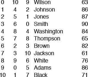
By manipulating indices, rather than the records themselves, we can sort an array simultaneously on several keys. For this sample data that might represent students’ names and grades, the second column is the result of an index sort on the name, and the third column is the result of an index sort on the grade. For example, Wilson is last in alphabetic order and has the tenth highest grade, while Adams is first in alphabetic order and has the sixth highest grade.
A rearrangement of the N distinct nonnegative integers less than N is called a permutation in mathematics: an index sort computes a permutation. In mathematics, permutations are normally defined as rearrangements of the integers 1 through N; we shall use 0 through N – 1 to emphasize the direct relationship between permutations and C array indices.
Figure 6.14 Index sorting example
This index-array approach to indirection will work in any programming language that supports arrays. Another possibility, especially attractive in C, is to use pointers. For example, defining the data type
typedef dataType *Item;
and then initializing a with
for (i = 0; i < N; i++) a[i] = &data[i];
and doing comparisons indirectly with
#define less(A, B) (*A < *B)
is equivalent to using the strategy described in the preceding paragraph. This arrangement is known as a pointer sort. The string data-type implementation that we just considered (Program 6.11) is an example of a pointer sort. For sorting an array of fixed-size items, a pointer sort is essentially equivalent to an index sort, but with the address of the array added to each index. But a pointer sort is much more general, because the pointers could point anywhere, and the items being sorted do not need to be fixed in size. As is true in index sorting, if a is an array of pointers to keys, then a call to sort will result in the pointers being rearranged such that accessing them sequentially will access the keys in order. We implement comparisons by following pointers; we implement exchanges by exchanging the pointers.
The standard C library sort function qsort is a pointer sort (see Program 3.17). The function takes four arguments: the array; the number of items to be sorted; the size of the items; and a pointer to a function that compares two items, given pointers to them. For example, if Item is char*, then the following code implements a string sort that adheres to our conventions:
int compare(void *i, void *j)
{ return strcmp(*(Item *)i, *(Item *)j); }
void sort(Item a[], int l, int r)
{ qsort(a, r-l+1, sizeof(Item), compare); }
The underlying algorithm is not specified in the interface, but quicksort (see Chapter 7) is widely used. In Chapter 7 we shall consider many of the reasons why this is true. We also, in this chapter and in Chapters 7 through 11, develop an understanding of why other methods might be more appropriate for some specific applications, and we explore approaches for speeding up the computation when the sort time is a critical factor in an application.
The primary reason to use indices or pointers is to avoid intruding on the data being sorted. We can “sort” a file even if read-only access is all that is available. Moreover, with multiple index or pointer arrays, we can sort one file on multiple keys (see Figure 6.14). This flexibility to manipulate the data without actually changing them is useful in many applications.
A second reason for manipulating indices is that we can avoid the cost of moving full records. The cost savings is significant for files with large records (and small keys), because the comparison needs to access just a small part of the record, and most of the record is not even touched during the sort. The indirect approach makes the cost of an exchange roughly equal to the cost of a comparison for general situations involving arbitrarily large records (at the cost of the extra space for the indices or pointers). Indeed, if the keys are long, the exchanges might even wind up being less costly than the comparisons. When we estimate the running times of methods that sort files of integers, we are often making the assumption that the costs of comparisons and exchanges are not much different. Conclusions based on this assumption are likely to apply to a broad class of applications, if we use pointer or index sorts.
In typical applications, the pointers are used to access records that may contain several possible keys. For example, records consisting of students’ names and grades or people’s names and ages:
struct record { char[30] name; int num; }
Programs 6.12 and 6.13 provide an example of a pointer sort interface and implementation that can allow us to sort them using either of the fields as key. We use an array of pointers to records, and declare less as a function, rather than a macro. Then we can provide different implementations of less for different sort applications. For example, if we compile Program 6.13 together with a file containing
#include "Item.h"
int less(Item a, Item b)
{ return a->num < b->num; }
then we get a data type for the items for which any of our sort implementations will do a pointer sort on the integer field. Alternatively, we might choose to use the string field of the records for the sort keys. If we compile Program 6.13 together with a file containing
#include <string.h>
#include "Item.h"
int less(Item a, Item b)
{ return strcmp(a->name, b->name) < 0; }
then we get a data type for the items for which any of our sort implementations will do a pointer sort on the string field.
For many applications, the data never need to be rearranged physically to match the order indicated by the indices, and we can simply access them in order using the index array. If this approach is not satisfactory for some reason, we are led to a classic programming exercise: How do we rearrange a file that has been sorted with an index sort? The code
for (i = 0; i < N; i++) datasorted[i] = data[a[i]];
is trivial, but requires extra memory sufficient for another copy of the array. What about the situation when there is not enough room for another copy of the file? We cannot blindly set data[i] = data[a[i]], because that would overwrite the previous value of data[i], perhaps prematurely.
Figure 6.15 illustrates how we can solve this problem, still using a single pass through the file. To move the first element where it belongs, we move the element at that position to where it belongs, and so forth. Continuing this reasoning, we eventually find an element to move to the first position, at which point we have shifted a cycle of elements into position. Then, we move to the second element and perform the same operation for its cycle, and so forth (any elements that we encounter that are already in position (a[i]=i) are on a cycle of length 1 and are not moved).

To rearrange an array in place, we move from left to right, moving elements that need to be moved in cycles. Here, there are four cycles: The first and last are single-element degenerate cases. The second cycle starts at 1. The S goes into a temporary variable, leaving a hole at 1. Moving the second A there leaves a hole at 10. This hole is filled by P, which leaves a hole at 12. That hole is to be filled by the element at position 1, so the reserved S goes into that hole, completing the cycle 1 10 12 that puts those elements in position. Similarly, the cycle 2 8 6 13 4 7 11 3 14 9 completes the sort.
Figure 6.15 In-place sort
Specifically, for each value of i, we save the value of data[i] and initialize an index variable k to i. Now, we think of a hole in the array at i, and seek an element to fill the hole. That element is data[a[k]]—in other words, the assignment data[k] = data[a[k]] moves the hole to a[k]. Now the hole is at data[a[k]], so we set k to a[k]. Iterating, we eventually get to a situation where the hole needs to be filled by data[i], which we have saved. When we move an element into position we update the a array to so indicate. Any element in position has a[i] equal to i, and the process just outlined is a no-op in that case. Continuing through the array, starting a new cycle each time that we encounter an element not yet moved, we move every element at most once. Program 6.14 is an implementation of this process.
This process is called in situ permutation, or in-place rearrangement of the file. Again, although the algorithm is interesting, it is unnecessary in many applications, because accessing the data indirectly often suffices. Also, if the records are huge relative to their number, the most efficient option may be simply to rearrange them with a conventional selection sort (see Property 6.5).
Indirect sorting requires extra space for the index or pointer array and extra time for the indirect comparisons. In many applications, these costs are a small price to pay for the flexibility of not having to move the data at all. For files consisting of large records, we will almost always choose to use an indirect sort, and for many applications, we will find that it is not necessary to move the data at all. In this book, we normally will access data directly. In a few applications, however, we do use pointers or index arrays to avoid data movement, for precisely the reasons mentioned here.
Exercises
6.56 Give an implementation of a data type for items where the items are records, rather than pointers to records. This arrangement might be preferable to Programs 6.12 and 6.13 for small records. (Remember that C supports structure assignment.)
![]() 6.57 Show how to use
6.57 Show how to use qsort to solve the sorting problem that is addressed in Programs 6.12 and 6.13.
![]() 6.58 Give the index array that results when the keys E A S Y Q U E S T I O N are index sorted.
6.58 Give the index array that results when the keys E A S Y Q U E S T I O N are index sorted.
![]() 6.59 Give the sequence of data moves required to permute the keys E A S Y Q U E S T I O N in place after an index sort (see Exercise 6.58).
6.59 Give the sequence of data moves required to permute the keys E A S Y Q U E S T I O N in place after an index sort (see Exercise 6.58).
6.60 Describe a permutation of size N (a set of values for the array a) that maximizes the number of times that a[i] != i during Program 6.14.
6.61 Prove that we are guaranteed to return to the key with which we started when moving keys and leaving holes in Program 6.14.
6.62 Implement a program like Program 6.14 corresponding to a pointer sort. Assume that the pointers point into an array of N records, of type Item.
6.9 Sorting of Linked Lists
As we know from Chapter 3, arrays and linked lists provide two of the most basic ways to structure data, and we considered an implementation of insertion sort for linked lists as a list-processing example in Section 3.4 (Program 3.11). The sort implementations that we have considered to this point all assume that the data to be sorted is in an array, and are not directly applicable if we are working within a system that uses linked lists to organize data. In some cases, the algorithms may be useful, but only if they process data in the essentially sequential manner that we can support efficiently for linked lists.
Program 6.15 gives an interface, which is similar to Program 6.7, for a linked-list data type. With Program 6.15, the driver program corresponding to Program 6.6 is a one-liner:
main(int argc, char *argv[])
{ show(sort(init(atoi(argv[1])))); }
Most of the work (including allocation of memory) is left to the linked-list and sort implementations. As we did with our array driver, we want to initialize the list (either from standard input or with random values), to show the contents of the list, and, of course, to sort it. As usual, we use an Item for the data type of the items being sorted, just as we did in Section 6.7. The code to implement the routines for this interface is standard for linked lists of the kind that we examined in detail in Chapter 3, and left as an exercise.
There is a ground rule for manipulating linked structures that is critical in many applications, but is not evident from this code. In a more complex environment, it could be the case that pointers to the list nodes that we are manipulating are maintained by other parts of the applications system (i.e., they are in multilists). The possibility that nodes could be referenced through pointers that are maintained outside the sort means that our programs should change only links in nodes, and should not alter keys or other information. For example, when we want to do an exchange, it would seem simplest just to exchange items (as we did when sorting arrays). But then any reference to either node with some other link would find the value changed, and probably will not have the desired effect. We need to change the links themselves such that the nodes appear in sorted order when the list is traversed via the links we have access to, without affecting their order when accessed via any other links. Doing so makes the implementations more difficult, but usually is necessary.
We can adapt insertion, selection, and bubble sort to linked-list implementations, although each one presents amusing challenges. Selection sort is straightforward: We maintain an input list (which initially has the data) and an output list (which collects the sorted result), and simply scan through the list to find the maximum element in the input list, remove it from the list, and add it to the front of the output list (see Figure 6.16). Implementing this operation is a simple exercise in linked-list manipulation, and is a useful method for sorting short lists. An implementation is given in Program 6.16. We leave the other methods for exercises.
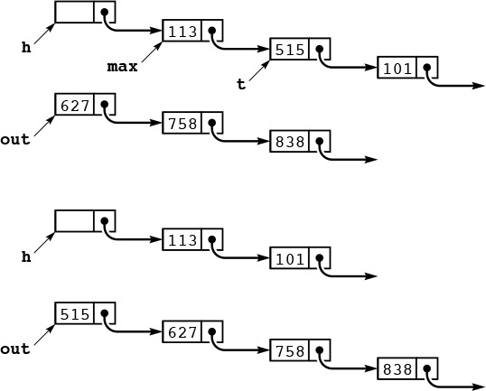
This diagram depicts one step of selection sort for linked lists. We maintain an input list, pointed to by h->next, and an output list, pointed to by out (top). We scan through the input list to make max point to the node before (and t point to) the node containing the maximum item. These are the pointers we need to remove t from the input list (reducing its length by 1) and put it at the front of the output list (increasing its length by 1), keeping the output list in order (bottom). Iterating, we eventually exhaust the input list and have the nodes in order in the output list.
Figure 6.16 Linked-list selection sort
In some list-processing situations, we may not need to explicitly implement a sort at all. For example, we could choose to keep the list in order at all times, inserting new nodes into the list as in insertion sort. This approach comes at little extra cost if insertions are relatively rare or the list is small, and in certain other situations. For example, we might need to scan the whole list for some reason before inserting new nodes (perhaps to check for duplicates). We shall discuss an algorithm that uses ordered linked lists in Chapter 14, and we shall see numerous data structures that gain efficiency from order in the data in Chapters 12 and 14.
Exercises
![]() 6.63 Give the contents of the input list and output list as Program 6.16 is used for the keys A S O R T I N G E X A M P L E.
6.63 Give the contents of the input list and output list as Program 6.16 is used for the keys A S O R T I N G E X A M P L E.
6.64 Provide an implementation for the linked-list interface given in Program 6.15.
6.65 Implement a performance-driver client program for linked-list sorts (see Exercise 6.9).
6.66 Implement bubble sort for a linked list. Caution: exchanging two adjacent elements on a linked list is more difficult than it seems at first.
![]() 6.67 Package the insertion-sort code in Program 3.11 such that it has the same functionality as Program 6.16.
6.67 Package the insertion-sort code in Program 3.11 such that it has the same functionality as Program 6.16.
6.68 The insertion-sort method used in Program 3.11 makes the linked-list insertion sort run significantly slower than the array version for some input files. Describe one such file, and explain the problem.
![]() 6.69 Implement a linked-list version of shellsort that does not use significantly more time or space than the array version for large random files. Hint: Use bubble sort.
6.69 Implement a linked-list version of shellsort that does not use significantly more time or space than the array version for large random files. Hint: Use bubble sort.
![]() 6.70 Implement an ADT for sequences, which allows us to use a single driver program to debug both linked-list and array sort implementations, for example with the following code:
6.70 Implement an ADT for sequences, which allows us to use a single driver program to debug both linked-list and array sort implementations, for example with the following code:
#include "Item.h"
#include "SEQ.h"
main(int argc, char *argv[])
{ int N = atoi(argv[1]), sw = atoi(argv[2]);
if (sw) SEQrandinit(N); else SEQscaninit(&N);
SEQsort();
SEQshow();
}
That is, client programs can create a sequence with N items (either generated randomly or filled from standard input), sort the sequence, or show its contents. Provide one implementation that uses an array representation and another that uses a linked-list representation. Use selection sort.
![]() 6.71 Extend your implementation from Exercise 6.70 such that it is a first-class ADT.
6.71 Extend your implementation from Exercise 6.70 such that it is a first-class ADT.
6.10 Key-Indexed Counting
A number of sorting algorithms gain efficiency by taking advantage of special properties of keys. For example, consider the following problem: Sort a file of N items whose keys are distinct integers between 0 and N – 1. We can solve this problem immediately, using a temporary array b, with the statement
for (i = 0; i < N; i++) b[key(a[i])] = a[i];
That is, we sort by using the keys as indices, rather than as abstract items that are compared. In this section, we consider an elementary method that uses key indexing in this way to sort efficiently when the keys are integers in a small range.
If all the keys are 0, sorting is trivial, but now suppose that there are two distinct key values 0 and 1. Such a sorting problem might arise when we want to separate out the items in a file that satisfy some (perhaps complicated) acceptance test: we take the key 0 to mean “accept” and the key 1 to mean “reject.” One way to proceed is to count the number of 0s, then to make a second pass through the input a to distribute its items to the temporary array b, using an array of two counters, as follows. We start with 0 in cnt[0] and the number of 0 keys in the file cnt[1], to indicate that there are no keys that are less than 0 and cnt[1] keys that are less than 1 in the file. Clearly, we can fill in the b array by putting 0s at the beginning (starting at b[[cnt[0]], or b[0]) and 1s starting at b[cnt[1]. That is, the code
for (i = 0; i < N; i++) b[cnt[a[i]]++] = a[i];
serves to distribute the items from a to b. Again, we get a fast sort by using the keys as indices (to pick between cnt[0] and cnt[1]). We could use an if statement to choose between the two counters in this simple case, but the approach of using keys as indices generalizes immediately to handle more than two key values (more than two counters).
Specifically, a more realistic problem in the same spirit is this: Sort a file of N items whose keys are integers between 0 and M – 1. We can extend the basic method in the previous paragraph to an algorithm called key-indexed counting, which solves this problem effectively if M is not too large. Just as with two key values, the idea is to count the number of keys with each value, and then to use the counts to move the items into position on a second pass through the file. First, we count the number of keys of each value: then, we compute partial sums to get counts of the number of keys less than or equal to each value. Then, again just as we did when we had two key values, we use these counts as indices for the purpose of distributing the keys. For each key, we view its associated count as an index pointing to the end of the block of keys with the same value, use the index to distribute the key into b, and decrement. The critical factor that makes this algorithm efficient is that we do not need to go through a chain of if statements to determine which counter to access—using the key as index, we immediately find the right one. This process is illustrated in Figure 6.17. An implementation is given in Program 6.17.
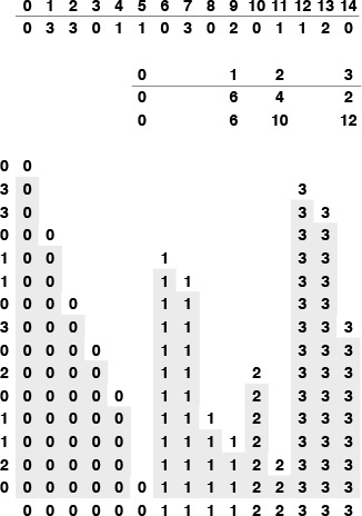
First, we determine how many keys of each value there are in the file: In this example there are six 0s, four 1s, two 2s, and three 3s. Then, we take partial sums to find the number of keys less than each key: 0 keys are less than 0, 6 keys are less than 1, 10 keys are less than 2, and 12 keys are less than 3 (table in middle). Then, we use the partial sums as indices in placing the keys into position: The 0 at the beginning of the file is put into location 0; we then increment the pointer corresponding to 0, to point to where the next 0 should go. Then, the 3 from the next position on the left in the file is put into location 12 (since there are 12 keys less than 3); its corresponding count is incremented; and so forth.
Figure 6.17 Sorting by key-indexed counting.
Property 6.12 Key-indexed counting is a linear-time sort, provided that the range of distinct key values is within a constant factor of the file size.
Each item is moved twice, once for the distribution and once to be moved back to the original array; and each key is referenced twice, once to do the counts and once to do the distribution. The two other for loops in the algorithm involve building the counts, and will contribute insignificantly to the running time unless the number of counts becomes significantly larger than the file size. ![]()
If huge files are to be sorted, the auxiliary array b can present memory-allocation problems. We can modify Program 6.17 to complete the sort in place (avoiding the need for an auxiliary array), using a method similar to that used in Program 6.14. This operation is closely related to the basic methods that we shall be discussing in Chapters 7 and 10, so we defer it to Exercises 12.16 and 12.17 in Section 12.3. As we shall see in Chapter 12, this space savings comes at the cost of the stability property of the algorithm, and thus limits the algorithm’s utility because applications involving large numbers of duplicate keys often have other associated keys, whose relative order should be preserved. We shall see a particularly important example of such an application in Chapter 10.
Exercises
![]() 6.72 Give a specialized version of key-indexed counting for sorting files where elements can take on only one of three values (a, b, or c).
6.72 Give a specialized version of key-indexed counting for sorting files where elements can take on only one of three values (a, b, or c).
6.73 Suppose that we use insertion sort on a randomly ordered file where elements have only one of three values. Is the running time linear, quadratic, or something in between?
![]() 6.74 Show how key-indexed counting sorts the file A B R A C A D A B R A.
6.74 Show how key-indexed counting sorts the file A B R A C A D A B R A.
6.75 Implement key-indexed counting for items that are potentially large records with integer keys from a small range.