5
SOME SPECIAL DISTRIBUTIONS
5.1 INTRODUCTION
In preceding chapters we studied probability distributions in general. In this chapter we will study some commonly occurring probability distributions and investigate their basic properties. The results of this chapter will be of considerable use in theoretical as well as practical applications. We begin with some discrete distributions in Section 5.2 and follow with some continuous models in Section 5.3. Section 5.4 deals with bivariate and multivariate normal distributions and in Section 5.5 we discuss the exponential family of distributions.
5.2 SOME DISCRETE DISTRIBUTIONS
In this section we study some well-known univariate and multivariate discrete distributions and describe their important properties.
5.2.1 Degenerate Distribution
The simplest distribution is that of an RV X degenerate at point k, that is, ![]() and = 0 elsewhere. If we define
and = 0 elsewhere. If we define
the DF of the RV X is ![]() . Clearly,
. Clearly, ![]() ,
, ![]() , and
, and ![]() . In particular,
. In particular, ![]() . This property characterizes a degenerate RV. As we shall see, the degenerate RV plays an important role in the study of limit theorems.
. This property characterizes a degenerate RV. As we shall see, the degenerate RV plays an important role in the study of limit theorems.
5.2.2 Two-Point Distribution
We say that an RV X has a two-point distribution if it takes two values, x 1 and x 2, with probabilities
We may write
where IA is the indicator function of A. The DF of X is given by
Also
In particular,
and
If ![]() ,
, ![]() , we get the important Bernoulli RV:
, we get the important Bernoulli RV:
For a Bernoulli RV X with parameter p, we write X ~ b(1, p) and have
Bernoulli RVs occur in practice, for example, in-coin-tossing experiments. Suppose that ![]() ,
, ![]() , and
, and ![]() . Define RV X so that
. Define RV X so that ![]() and
and ![]() . Then
. Then ![]() and
and ![]() . Each repetition of the experiment will be called a trial. More generally, any nontrivial experiment can be dichotomized to yield a Bernoulli model. Let (Ω,
. Each repetition of the experiment will be called a trial. More generally, any nontrivial experiment can be dichotomized to yield a Bernoulli model. Let (Ω, ![]() , P) be the sample space of an experiment, and let
, P) be the sample space of an experiment, and let ![]() with
with ![]() . Then
. Then ![]() . Each performance of the experiment is a Bernoulli trial. It will be convenient to call the occurrence of event A a success and the occurrence of Ac, a failure.
. Each performance of the experiment is a Bernoulli trial. It will be convenient to call the occurrence of event A a success and the occurrence of Ac, a failure.
5.2.3 Uniform Distribution on n Points
X is said to have a uniform distribution on n points {x 1, x 2, … , xn } if its PMF is of the form
Thus we may write


and

if we write ![]() . Also,
. Also,

If, in particular, ![]() ,
,


5.2.4 Binomial Distribution
We say that X has a binomial distribution with parameter p if its PMF is given by

Since ![]() , the pk
’s indeed define a PMF. If X has PMF (17), we will write X ~ b(n, p). This is consistent with the notation for a Bernoulli RV. We have
, the pk
’s indeed define a PMF. If X has PMF (17), we will write X ~ b(n, p). This is consistent with the notation for a Bernoulli RV. We have

In Example 3.2.5 we showed that
and
where ![]() . Also
. Also

The PGF of ![]() is given by
is given by ![]() .
.
Binomial distribution can also be considered as the distribution of the sum of n independent, identically distributed b (1, p) random variables. If we toss a coin, with constant probability p of heads and 1 − p of tails, n times, the distribution of the number of heads is given by (17). Alternatively, if we write

the number of heads in n trials is the sum ![]() . Also
. Also
Thus

and

5.2.5 Negative Binomial Distribution (Pascal or Waiting Time Distribution)
Let (Ω, ![]() , P) be a probability space of a given statistical experiment, and let
, P) be a probability space of a given statistical experiment, and let ![]() with
with ![]() . On any performance of the experiment, if A happens we call it a success, otherwise a failure. Consider a succession of trials of this experiment, and let us compute the probability of observing exactly r successes, where
. On any performance of the experiment, if A happens we call it a success, otherwise a failure. Consider a succession of trials of this experiment, and let us compute the probability of observing exactly r successes, where ![]() is a fixed integer. If X denotes the number of failures that precede the rth success,
is a fixed integer. If X denotes the number of failures that precede the rth success, ![]() is the total number of replications needed to produce r successes. This will happen if and only if the last trial results in a success and among the previous
is the total number of replications needed to produce r successes. This will happen if and only if the last trial results in a success and among the previous ![]() trials there are exactly X failures. It follows by independence that
trials there are exactly X failures. It follows by independence that
Rewriting (22) in the form
we see that

It follows that

Let X be a b(n, p) RV, and let Y be the RV defined in (28). If there are r or more successes in the first n trials, at most n trials were required to obtain the first r of these successes.
We have
and also
In the special case when ![]() , the distribution of X is given by
, the distribution of X is given by
An RV X with PMF (33) is said to have a geometric distribution. Clearly, for the geometric distribution, we have

5.2.6 Hypergeometric Distribution
A box contains N marbles. Of these, M are drawn at random, marked, and returned to the box. The contents of the box are then thoroughly mixed. Next, n marbles are drawn at random from the box, and the marked marbles are counted. If X denotes the number of marked marbles, then

Since x cannot exceed M or n, we must have
Also ![]() and
and ![]() , so that
, so that
Note that

for arbitrary numbers a, b and positive integer n. It follows that

5.2.7 Negative Hypergeometric Distribution
Consider the model of Section 5.2.6. A box contains N marbles, M of these are marked (or say defective) and ![]() are unmarked. A sample of size n is taken and let X denote the number of defective marbles in the sample. If the sample is drawn without replacement we saw that X has a hypergeometric distribution with PMF (40). If, on the other hand, the sample is drawn with replacement then
are unmarked. A sample of size n is taken and let X denote the number of defective marbles in the sample. If the sample is drawn without replacement we saw that X has a hypergeometric distribution with PMF (40). If, on the other hand, the sample is drawn with replacement then ![]() where
where ![]() .
.
Let Y denote the number of draws needed to draw the rth defective marble. If the draws are made with replacement then Y has the negative binomial distribution given in (22) with ![]() . What if the draws are made without replacement? In that case in order that the kth draw (
. What if the draws are made without replacement? In that case in order that the kth draw (![]() ) be the rth defective marble drawn, the kth draw must produce a defective marble, whereas the previous
) be the rth defective marble drawn, the kth draw must produce a defective marble, whereas the previous ![]() draws must produce
draws must produce ![]() defectives. It follows that
defectives. It follows that

for ![]() . Rewriting we see that
. Rewriting we see that

An RV Y with PMF (50) is said to have a negative hypergeometric distribution.
It is easy to see that
and
Also, if ![]() , and
, and ![]() as
as ![]() , then
, then

which is (22).
5.2.8 Poisson Distribution
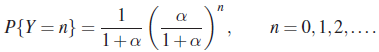
Remark 2. The converse of this result is also true in the following sense. If X and Y are independent nonnegative integer-valued RVs such that ![]() ,
, ![]() , for k = 0,1, 2, … , and the conditional distribution of X, given
, for k = 0,1, 2, … , and the conditional distribution of X, given ![]() , is binomial, both X and Y are Poisson. This result is due to Chatterji [13]. For the proof see Problem 13.
, is binomial, both X and Y are Poisson. This result is due to Chatterji [13]. For the proof see Problem 13.
5.2.9 Multinomial Distribution
The binomial distribution is generalized in the following natural fashion. Suppose that an experiment is repeated n times. Each replication of the experiment terminates in one of k mutually exclusive and exhaustive events A1, A2, …, Ak. Let pj be the probability that the experiment terminates in Aj, ![]() , and suppose that pj (
, and suppose that pj (![]() ) remains constant for all n replications. We assume that the n replications are independent.
) remains constant for all n replications. We assume that the n replications are independent.
Let x1, x2, …, xk−1 be nonnegative integers such that ![]() . Then theprobability that exactly xi
trials terminate in Ai,
. Then theprobability that exactly xi
trials terminate in Ai, ![]() and hence that
and hence that ![]() trials terminate in Ak
is clearly
trials terminate in Ak
is clearly
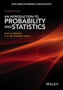
If (X1, X2,…, Xk) is a random vector such that Xj = xj means that event Aj has occurred xj times, xj = 0,1, 2, …, n, the joint PMF of (X1, X2, …, Xk) is given by

From the MGF of (X1, X2, … , Xk−1) or directly from the marginal PMFs we can compute the moments. Thus
and for ![]() , and
, and ![]() ,
,
It follows that the correlation coefficient between Xi and Xj is given by

Finally, we note that, if ![]() and
and ![]() are two independent multinomial RVs with common parameter (p1, p2, … , pk), then
are two independent multinomial RVs with common parameter (p1, p2, … , pk), then ![]() is also a multinomial RV with probabilities (p1, p2, … , pk). This follows easily if one employs the MGF technique, using (57). Actually this property characterizes the multinomial distribution. If X and Y are k-dimensional, nonnegative, independent random vectors, and if
is also a multinomial RV with probabilities (p1, p2, … , pk). This follows easily if one employs the MGF technique, using (57). Actually this property characterizes the multinomial distribution. If X and Y are k-dimensional, nonnegative, independent random vectors, and if ![]() is a multinomial random vector with parameter (p
1
, p
2, … , pk
), then X and Y also have multinomial distribution with the same parameter. This result is due to Shanbhag and Basawa
[103]
and will not be proved here.
is a multinomial random vector with parameter (p
1
, p
2, … , pk
), then X and Y also have multinomial distribution with the same parameter. This result is due to Shanbhag and Basawa
[103]
and will not be proved here.
5.2.10 Multivariate Hypergeometric Distribution
Consider an urn containing N items divided into k categories containing n
1, n
2, … , nk
items, where ![]() . A random sample, without replacement, of size n is taken from the urn. Let Xi = number of items in sample of type i. Then
. A random sample, without replacement, of size n is taken from the urn. Let Xi = number of items in sample of type i. Then
where ![]() and
and ![]()
We say that (X 1, X 2 , … , X k−1) has multivariate hypergeometric distribution if its joint PMF is given by (65). It is clear that each Xj has a marginal hypergeometric distribution. Moreover, the conditional distributions are also hypergeometric. Thus

and

and so on. It is therefore easy to write down the marginal and conditional means and variances. We leave the reader to show that

and
5.2.11 Multivariate Negative Binomial Distribution
Consider the setup of Section 5.2.9 where each replication of an experiment terminates in one of k mutually exclusive and exhaustive events A
1, A
2, … , Ak
.Let ![]() , j = 1, 2, … , k. Suppose the experiment is repeated until event Ak
is observed for the rth time,
, j = 1, 2, … , k. Suppose the experiment is repeated until event Ak
is observed for the rth time, ![]() . Then
. Then

for ![]() ,
, ![]() ,
, ![]() ,
, ![]() , and
, and ![]() .
.
We say that (X 1, X 2, … , X k−1) has a multivariate negative binomial (or negative multinomial) distribution if its joint PMF is given by (66).
It is easy to see the marginal PMF of any subset of {X 1 , X 2 , … , X k–1} is negative multinomial. In particular, each Xj has a negative binomial distribution.
We will leave the reader to show that

and

PROBLEMS 5.2
-
- Let us write

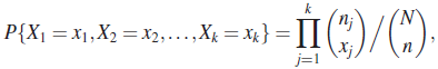
Show that, as k goes 0 to n, b(k; n, p) first increases monotonically and then decreases monotonically. The greatest value is assumed when
 , where m is an integer such that
except that
 when
when  .
. - If
 , then
and if
 , then
- Let us write
- Generalize the result in Theorem 10 to n independent Poisson RVs, that is, if X1, X2, … , Xn are independent RVs with
 , the conditional distribution of X
1, X
2,…Xn
given
, the conditional distribution of X
1, X
2,…Xn
given  , is multinomial with parameters t,
  .
. - Let X
1, X
2 be independent RVs with
 . What is the PMF of
  ?
? - A box contains N identical balls numbered 1 through N. Of these balls, n are drawn at a time. Let X
1, X
2, … , Xn
denote the numbers on the n balls drawn. Let
 . Find var(Sn
).
. Find var(Sn
). - From a box containing N identical ball marked 1 through N, M balls are drawn one after another without replacement. Let Xi
denote the number on the ith ball drawn,
 ,
,  . Let
. Let  . Find the DF and the the PMF of Y. Also find the conditional distribution of X1, X2, … , XM given Y = y. Find EY and var(Y).
 - Let f(x; r, p),
 , denote the PMF of an NB(r; p) RV. Show that the terms f(x; r, p) first increase monotonically and then decrease monotonically. When is the greatest value assumed?
 - Show that the terms

of the Poisson PMF reach their maximum when k is the largest integer ≤ λ and at (λ – 1) and λ if λ is an integer.
- Show that

as n → ∞ and p → 0, so that np = λ remains constant.
[Hint: Use Stirling’s approximation, namely,
 as n → ∞.]
 - A biased coin is tossed indefinitely. Let p(0 < p < 1) be the probability of success (heads). Let Y 1 denote the length of the first run, and Y 2, the length of the second run. Find the PMFs of Y 1 and Y 2 and show that EY 1 = q/p + p/q, EY 2 = 2. If Yn denotes the length of the nth run, n ≥ 1, what is the PMF of Yn ? Find EYn .
- Show that

as N → ∞.
- Show that

as p → 1 and r → ∞ in such a way that r(1 – p) = λ remains fixed.
- Let X and Y be independent geometric RVs. Show that min (X, Y) and X – Y are independent.
- Let X and Y be independent RVs with PMFs
 , 1, 2, … , where pk
, qk
> 0 and
, 1, 2, … , where pk
, qk
> 0 and  . Let
. Let
Then αt = α for all t, and

where
 , and - θ > 0 is arbitrary.
(Chatterji [13])
- Generalize the result of Example 10 to the case of k urns, k ≥ 3.
- Let (X
1, X
2, … , X
k–1) have a multinomial distribution with parameters n, p
1, p
2, … , p
k−1. Write

where pk = 1 – p 1 –
 – p
k–1, and
– p
k–1, and  . Find EY and var(Y).
 - Let X
1, X
2 be iid RVs with common DF F, having positive mass at 0, 1, 2,… Also, let U = max(X
1, X
2) and
 . Then
For all j if and only if F is a geometric distribution.
(Srivastava [109])
- Let X and Y be mutually independent RVs, taking nonnegative integer values. Then

Holds for n = 0, 1, 2,… and some α > 0 if and only if
[Hint: Use Problem 3.3.8.]
(Puri [83])
- Let X1, X2,… be a sequence of independent b(1, p) RVs with
 . Also, let
  , where N is a P(λ) RV which is independent of the Xi
’s. Show that ZN
and N – ZN
are independent.
, where N is a P(λ) RV which is independent of the Xi
’s. Show that ZN
and N – ZN
are independent. - Prove Theorems 5, 7, 8 and 11.
- In Example 2 show that

5.3 SOME CONTINUOUS DISTRIBUTIONS
In this section we study some most frequently used absolutely continuous distributions and describe their important properties. Before we introduce specific distributions it should be remarked that associated with each PDF f there is an index or a parameter θ (may be multidimensional) which takes values in an index set Θ. For any particular choice of θ ∈ Θ we obtain a specific PDF fθ from the family of PDFs {fθ , θ ∈ Θ}.
Let X be an RV with PDF fθ
(x), where θ is a real-valued parameter. We say that θ is a location parameter and {fθ
} is a location family if X – θ has PDF f(x) which does not depend on θ. The parameter θ is said to be a scale parameter and {fθ
} is a scale family of PDFs if X/θ has PDF f(x) which is free of θ. If ![]() is two-dimensional, we say that θ is a location-scale parameter if the PDF of (X–μ)/σ is free of μ and σ. In that case {fθ
} is known as a location-scale family.
is two-dimensional, we say that θ is a location-scale parameter if the PDF of (X–μ)/σ is free of μ and σ. In that case {fθ
} is known as a location-scale family.
It is easily seen that θ is a location parameter if and only if ![]() , a scale parameter if and only
, a scale parameter if and only ![]() , and a location-scale parameter if
, and a location-scale parameter if ![]() ,
, ![]() for some PDF f. The density f is called the standard PDF for the family {fθ, θ ∈ Θ}.
for some PDF f. The density f is called the standard PDF for the family {fθ, θ ∈ Θ}.
A location parameter simply relocates or shifts the graph of PDF f without changing its shape. A scale parameter stretches (if ![]() ) or contracts (if
) or contracts (if ![]() ) the graph of f. A location-scale parameter, on the other hand, stretches or contracts the graph of f with the scale parameter and then shifts the graph to locate at μ. (see Fig. 1.)
) the graph of f. A location-scale parameter, on the other hand, stretches or contracts the graph of f with the scale parameter and then shifts the graph to locate at μ. (see Fig. 1.)


Fig. 1 (a) Exponential location family; (b) exponential scale family; (c) normal location-scale family; and (d) shaped parameter family  .
.
Some PDFs also have a shape parameter. Changing its value alters the shape of the graph. For the Poisson distribution λ is a shape parameter.
For the following PDF

and = 0 otherwise, μ is a location, β, a scale, and α, a shape parameter. The standard density for this location-scale family is
and = 0 otherwise. For the standard PDF f, α is a shape parameter.
5.3.1 Uniform Distribution (Rectangular Distribution)
Indeed, ![]() implies, that, for every
implies, that, for every ![]() ,
, ![]() . Since
. Since ![]() is arbitrary and F is continuous on the right, we let ε → 0 and conclude that
is arbitrary and F is continuous on the right, we let ε → 0 and conclude that ![]() . Since
. Since ![]() implies
implies ![]() by definition (7), it follows that (8) holds generally. Thus
by definition (7), it follows that (8) holds generally. Thus
Theorem 2 is quite useful in generating samples with the help of the uniform distribution.
To complete the proof we consider the case where x is a positive irrational number. Then we can find a decreasing of positive rational x 1, x 2,… such that xn → x. Since f is right continuous,
Now, for ![]() ,
,

Since ![]() , we must have
, we must have ![]() , so that
, so that
This complete the proof.
5.3.2 Gamma Distribution
The integral

converges or diverges according as ![]() or ≤ 0. For
or ≤ 0. For ![]() the integral in (9) is called the gamma function. In particular, if
the integral in (9) is called the gamma function. In particular, if ![]() ,
, ![]() . If
. If ![]() , integration by parts yields
, integration by parts yields

If ![]() is a positive integer, then
is a positive integer, then
Also writing ![]() in
in ![]() we see that
we see that

Now consider the integral  . We have

and changing to polar coordinates we get

It follows that ![]()
Let us write ![]() ,
, ![]() , in the integral in (9). Then
, in the integral in (9). Then

so that

Since the integrand in (13) is positive for ![]() , it follows that the function
, it follows that the function

defines a PDF for ![]() ,
, ![]()
The special case when ![]() leads to the exponential distribution with parameter β. The PDF of an exponentially distributed RV is therefore
leads to the exponential distribution with parameter β. The PDF of an exponentially distributed RV is therefore

Note that we can speak of the exponential distribution on (−∞, 0). The PDF of such an RV is

Clearly, if ![]() , we have
, we have
Another special case of importance is when ![]() ,
, ![]() (an integer), and
(an integer), and ![]() .
.
If X ~ χ2(n), then
and
5.3.3 Beta Distribution
The integral

converges for ![]() and
and ![]() and is called a beta function. For
and is called a beta function. For ![]() or
or ![]() the integral in (37) diverges. It is easy to see that for
the integral in (37) diverges. It is easy to see that for ![]() and
and ![]()
and

and
It follows that
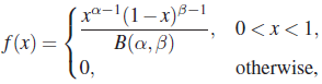
defines a pdf.
Let X1,X2,…,Xn be iid RVs with the uniform distribution on [0, 1]. Let X(k) be the kth-order statistic.
5.3.4 Cauchy Distribution
We will write ![]() for a Cauchy RV with density (49)
for a Cauchy RV with density (49)
Figure 4 gives graph of a Cauchy PDF.

Fig. 4 Cauchy density function.
We first check that (49) in fact defines a PDF. Substituting ![]() , we get
, we get

The DF of a ![]() (1, 0) RV is given by
(1, 0) RV is given by
It follows from Theorem 17 that the MGF of a Cauchy RV does not exist. This creates some manipulative problems. We note, however, that the CF of ![]() is given by
is given by
In particular, if X
1,X2, … , Xn
are iid ![]() (1,0) RVs, n—1Sn
is also a
(1,0) RVs, n—1Sn
is also a ![]() (1,0) RV. This is a remarkable result, the importance of which will become clear in Chapter 7. Actually, this property uniquely characterizes the Cauchy distribution. If F is a nondegenerate DF with the property that n-1Sn
also has DF F, then F must be a Cauchy distribution (see Thompson [113, p. 112]).
(1,0) RV. This is a remarkable result, the importance of which will become clear in Chapter 7. Actually, this property uniquely characterizes the Cauchy distribution. If F is a nondegenerate DF with the property that n-1Sn
also has DF F, then F must be a Cauchy distribution (see Thompson [113, p. 112]).
The proof of the following result is simple.
We emphasize that if X and 1 /X have the same PDF on (−∞,∞), it does not follow* that X is ![]() (1,0), for let X be an RV with PDF
(1,0), for let X be an RV with PDF

Then X and 1 /X have the same PDF, as can be easily checked.
5.3.5 Normal Distribution (the Gaussian Law)
One of the most important distributions in the study of probability and mathematical statistics is the normal distribution, which we will examine presently.
If X is a normally distributed RV with parameters μ and σ, we will write ![]() . In this notation φ defined by (53) is the PDF of an
. In this notation φ defined by (53) is the PDF of an ![]() (0,1) RV. The DF of an
(0,1) RV. The DF of an ![]() (0, 1) RV will be denoted Φ (x), where
(0, 1) RV will be denoted Φ (x), where

Clearly, if ![]() , then
, then ![]() . Z is called a standard normal RV. For the MGF of an
. Z is called a standard normal RV. For the MGF of an ![]() RV, we have
RV, we have

for all real values of t. Moments of all order exist and may be computed from the MGF. Thus
and

Thus
Clearly, the central moments of odd order are all 0. The central moments of even order are as follows:

As for the absolute moment of order α, for a standard normal RV Z we have

As remarked earlier, the normal distribution is one of the most important distributions in probability and statistics, and for this reason the standard normal distribution is available in tabular form. Table ST2 at the end of the book gives the probability ![]() for various values of
for various values of ![]() in the tail of an
in the tail of an ![]() RV. In this book we will write za
for the value of Z that satisfies
RV. In this book we will write za
for the value of Z that satisfies ![]() .
.
We remark that if X1, X2, … , Xn are iid RVs with ![]() such that
such that ![]() also has the same distribution for each
also has the same distribution for each ![]() , that distribution can only be
, that distribution can only be ![]() (0,1). This characterization of the normal distribution will become clear when we study the central limit theorem in Chapter 7.
(0,1). This characterization of the normal distribution will become clear when we study the central limit theorem in Chapter 7.
If X and Y are independent normal RVs, ![]() is normal by Theorem 22. The converse is due to Cramér
[16]
and will not be proved here.
is normal by Theorem 22. The converse is due to Cramér
[16]
and will not be proved here.
In Chapter 6 we will prove the necessity part of this result, which is basic to the theory of t-tests in statistics (Chapter 10; see also Example 4.4.6). The sufficiency part was proved by Lukacs [67] , and we will not prove it here.
We remark that the converse of this result does not hold; that is, if ![]() is the quotient of two iid RVs and Z has a
is the quotient of two iid RVs and Z has a ![]() (1, 0) distribution, it does not follow that X and Y are normal, for take X and Y to be iid with PDF
(1, 0) distribution, it does not follow that X and Y are normal, for take X and Y to be iid with PDF

We leave the reader to verify that ![]() is
is ![]() (1, 0).
(1, 0).
5.3.6 Some Other Continuous Distributions
Several other distributions which are related to distributions studied earlier also arise in practice. We record briefly some of these and their important characteristics. We will use these distributions infrequently. We say that X has a lognormal distribution if ![]() X has a normal distribution. The PDF of X is then
X has a normal distribution. The PDF of X is then

and ![]() for
for ![]() , where
, where ![]() . In fact for
. In fact for ![]()

Where Φ is the DF of a ![]() (0, 1) RV which leads to (65). It is easily seen that for n≥0
(0, 1) RV which leads to (65). It is easily seen that for n≥0
The MGF of X does not exist.
We say that the RV X has a Pareto distribution with parameters ![]() and
and ![]() if its PDF is given by
if its PDF is given by
and 0 otherwise. Here θ is scale parameter and α is a shape parameter. It is easy to check that

for α > 2. The MGF of X does not exist since all moments of X do not.
Suppose X has a Pareto distribution with parameters θ and α. Wright ![]() we see that Y has PDF
we see that Y has PDF

and DF
The PDF in (69) is known as a logistic distribution. We introduce location and scale parameters μ and σ by writing ![]() taking
taking ![]() and then the PDF of Z is easily seen
and then the PDF of Z is easily seen
to be

for all real z. This is the PDF of a logistic RV with location-scale parameters μ and σ. We leave the reader to check that

Pareto distribution is also related to an exponential distribution. Let X have Pareto PDF of the form
and 0 otherwise. A simple transformation leads to PDF (72) from (67). Then it is easily seen that ![]() has an exponential distribution with mean 1/α. Thus some properties of exponential distribution which are preserved under monotone transformations can be derived for Pareto PDF (72) by using the logarithmic transformation.
has an exponential distribution with mean 1/α. Thus some properties of exponential distribution which are preserved under monotone transformations can be derived for Pareto PDF (72) by using the logarithmic transformation.
Some other distributions are related to the gamma distribution. Suppose ![]() .
.
Let ![]() . Then Y has PDF
. Then Y has PDF
and 0 otherwise. The RV Y is said to have a Weibull distribution. We leave the reader to show that

The MGF of Y exists only for ![]() but for
but for ![]() it does not have a form useful in applications. The special case
it does not have a form useful in applications. The special case ![]() and
and ![]() is known as a Rayleigh distribution.
is known as a Rayleigh distribution.
Suppose X has a Weibull distribution with PDF (73). Let ![]() . Then Y has DF
. Then Y has DF
Setting ![]() and
and ![]() we get
we get

with PDF

for ![]() and
and ![]() . An RV with PDF (76) is called an extreme value distribution with location-scale parameters θ and σ. It can be shown that
. An RV with PDF (76) is called an extreme value distribution with location-scale parameters θ and σ. It can be shown that

where ![]() is the Euler constant.
is the Euler constant.
The final distribution we consider is also related to a G(1, β) RV. Let f 1 be the PDF of G(1, β) and f 2 the PDF

Clearly f
2 is also an exponential PDF defined on ![]() . Consider the mixture PDF
. Consider the mixture PDF
Clearly,
and the PDF f defined in (79) is called a Laplace or double exponential pdf. It is convenient to introduce a location parameter μ and consider instead the PDF

where ![]() . It is easy to see that for RV X with PDF (80) we have
. It is easy to see that for RV X with PDF (80) we have
for ![]() .
.
For completeness let us define a mixture PDF (PMF). Let ![]() be a PDF and let h(θ) be a mixing PDF. Then the PDF
be a PDF and let h(θ) be a mixing PDF. Then the PDF
is called a mixture density function. In case h is a PMF with support set {θ1, θ2, …, θ κ }, then (82) reduces to a finite mixture density function

The quantities h(θ
i
) are called mixing proportions. The PDF (78) is an example with ![]() , and
, and ![]() .
.
PROBLEMS 5.3
- Prove Theorem 1.
- Let X be an RV with PMF
 given below. If F is the corresponding DF, find the distribution of F(X), in the following cases:
- Let
 . Show that
where X 1, X 2, … , X n are iid U[0,1] RVs. If U is the number of Y1, Y 2 , … , Yn in [t, 1], where
 , show that U has a Poisson distribution with parameter – log t.
 - Let X
1,
X
2, … , X
n
be iid U[0,1] RVs. Prove by induction or otherwise that
 has the PDF
where
 if
if  if
if  .
. -
- Let X be an RV with PMF
 ,
,  , and let F be the DF of X. Show that
where
 .
. - Let
 for
for  and
and  .
Show that
.
Show that
with equality if and only if
 for all j.
- Let X be an RV with PMF
- Prove (a) Theorem 6 and its corollary, and (b) Theorem 10.
- Let X be a nonnegative RV of the continuous type, and let
 . Also, let
  . Then the RVs Y and Z are independent if and only if X is G(2, 1/λ) for some
  .
.
(Lamperti [59])
- Let X and Y be independent RVs with common PDF
 if
if  , and = 0 otherwise;
  . Let
. Let  and
and  . Find the joint PDF of U and V and the PDF of
  . Show that U/V and V are independent.
 - Prove Theorem 14.
- Prove Theorem 8.
- Prove Theorems 19 and 20.
- Let X
1, X
2
, … , Xn
be independent RVs with
 ,
,  . Show that the RV
  is also a Cauchy RV with parameters
  and
and  , where
- Let X1, X2, … , Xn be iid
 (1,0) RVs and
  , bi
,
, bi
,  , be any real numbers. Find the distribution of
  .
.
- Suppose that the load of an airplane wing is a random variable X with
 (1000, 14400) distribution. The maximum load that the wing can withstand is an RV Y, which is (1260,2500). If X and Y are independent, find the probability that the load encountered by the wing is less than its critical load.
 - Let X ~ (0,1). Find the PDF of
 . If X and Y are iid (0,1), deduce that
  is (0,1/4).
 - In Problem 15 let X and Y be independent normal RVs with zero means. Show that
 is normal. If, in addition,
  show that
  is also normal. Moreover, U and V are independent.
(Shepp [104] )
- Let X
1
,X
2
,X
3
,X
4 be independent (0,1). Show that
 has the PDF
  ,
,  .
. - Let X ~ (15,16). Find (a)
 , (b)
, (b)  , (c)
, (c)  and (d)
  .
. - Let X ~ (−1, 9). Find x such that
 . Also find x such that
  .
. - Let X be an RV such that
 is (μ, σ2). Show that X has PDF
If m 1, m 2 are the first two moments of this distribution and
 is the coefficient of skewness, show that a, μ, σ are given by
and

where η is the real root of the equation
 .
. - Let
 and let
  .
.
- Find the PDF of Y.
- Find the conditional PDF of X given
 .
. - Find
 .
.
- Let X and Y be iid (0,1) RVs. Find the PDF of X/|Y|. Also, find the PDF of |X|/|Y|.
- It is known that
 and
and  . If
. If  , find α and β.
[Hint: Use Table ST1.]
- Let X
1
, X
2
, … , Xn
be iid (μ, σ2) RVs. Find the distribution of

- Let F 1, F 2 , … , Fn be n DFs. Show that min[F 1(x 1),F 2(x 2), … , Fn (xn )] is an n-dimensional DF with marginal DFs F 1, F 2 , …Fn. (Kemp [50] )
- Let X ~ NB(1;p) and Y ~ G(1, 1/λ). Show that X and Y are related by the equation

where [x] is the largest integer ≤ x. Equivalently, show that

where

(Prochaska [82]).
- Let T be an RV with DF F and write
 . The function F is called the survival (or reliability) function of X (or DF F). The function
  is called hazard (or failure-rate) function. For the following PDF find the hazard function:
- Rayleigh:
 .
. - Lognormal:
 .
. - Pareto:
 ,
,  , and = 0 otherwise.
 - Weibull:
 ,
,  .
. - Logistic:
 ,
,  .
.
- Rayleigh:
- Consider the PDF
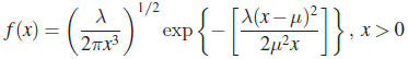
and = 0 otherwise. An RV X with PDF f is said to have an inverse Gaussian distribution with parameters μ and λ, both positive. Show that

- Let f be the PDF of a (μ, σ
2) RV:
- For what value of c is the function cfn, n > 0, a pdf?
- Let Φ be the DF of Z ~ (0,1). Find E{Z Φ (Z)} and E{Z2 Φ (Z)}.
5.4 BIVARIATE AND MULTIVARIATE NORMAL DISTRIBUTIONS
In this section we introduce the bivariate and multivariate normal distributions and investigate some of their important properties. We note that bivariate analogs of other PDFs are known but they are not always uniquely identified. For example, there are several versions of bivariate exponential PDFs so-called because each has exponential marginals. We will not encounter any of these bivariate PDFs in this book.
We first show that (1) indeed defines a joint PDF. In fact, we prove the following result.
Furthermore, we have

where βx
is given by (4). It is clear, then, that the conditional PDF ![]() given by (5) is also normal, with parameters βx
and
given by (5) is also normal, with parameters βx
and ![]() . We have
. We have
and
In order to show that ρ is the correlation coefficient between X and Y, it suffices to show that ![]() . We have from (6)
. We have from (6)

It follows that
Remark 1. If ρ2 = 1, then (1) becomes meaningless. But in that case we know (Theorem 4.5.1) that there exist constants a and b such that ![]() . We thus have a univariate distribution, which is called the bivariate degenerate (or singular) normal distribution. The bivariate degenerate normal distribution does not have a PDF but corresponds to an RV (X, Y) whose marginal distributions are normal or degenerate and are such that (X, Y) falls on a fixed line with probability 1. It is for this reason that degenerate distributions are considered as normal distributions with variance 0.
. We thus have a univariate distribution, which is called the bivariate degenerate (or singular) normal distribution. The bivariate degenerate normal distribution does not have a PDF but corresponds to an RV (X, Y) whose marginal distributions are normal or degenerate and are such that (X, Y) falls on a fixed line with probability 1. It is for this reason that degenerate distributions are considered as normal distributions with variance 0.
Next we compute the MGF M(t 1 , t 2) of a bivariate normal RV (X, Y). We have, if f(x, y) is the PDF given in (1) and f 1 is the marginal PDF of X,

Now

Therefore

The following result is an immediate consequence of (8).
In particular, take f and g to be the PDF of ![]() (0,1), that is,
(0,1), that is,
and let (X, Y) have the joint PDF h(x, y). We will show that ![]() is not normal except in the trivial case
is not normal except in the trivial case ![]() , when X and Y are independent.
, when X and Y are independent.
Let ![]() . Then
. Then
It is easy to show (Problem 2) that cov ![]() , so that var
, so that var ![]() . If Z is normal, its MGF must be
. If Z is normal, its MGF must be
Next we compute the MGF of Z directly from the joint PDF (10). We have

Now

Where Z1 is an ![]() (0, 1) RV
(0, 1) RV
It follows that
If Z were normally distributed, we must have ![]() for all t and all
for all t and all ![]() , that is,
, that is,

For ![]() , the equality clearly holds. The expression within the brackets on the right side of (15) is bounded by
, the equality clearly holds. The expression within the brackets on the right side of (15) is bounded by ![]() , whereas the expression r
(α/π)t2 is unbounded, so the equality cannot hold for all t and α.
, whereas the expression r
(α/π)t2 is unbounded, so the equality cannot hold for all t and α.
Next we investigate the multivariate normal distribution of dimension n, ![]() . Let M be an n × n real, symmetric, and positive definite matrix. Let x denote the n × 1 column vector of real numbers (x
1, x
2, … , xn
)' and let
μ
denote the column vector (μ
1, μ
2, … , μn
)', where
. Let M be an n × n real, symmetric, and positive definite matrix. Let x denote the n × 1 column vector of real numbers (x
1, x
2, … , xn
)' and let
μ
denote the column vector (μ
1, μ
2, … , μn
)', where ![]() are real constants.
are real constants.
Since M is positive definite, it follows that all the n characteristic roots of M, say m
1
, m
2, … ,
mn, are positive. Moreover, since M is symmetric there exists an n × n orthogonal matrix L such that L′ML is a diagonal matrix with diagonal elements m
1
, m
2
, … , mn. Let us change the variables to z1, z
2
, … , zn
by writing ![]() where
where ![]() , and note that the Jacobian of this orthogonal transformation is |L|. Since
, and note that the Jacobian of this orthogonal transformation is |L|. Since ![]() , where In is an n × n unit matrix,
, where In is an n × n unit matrix, ![]() and we have
and we have

If we write ![]() then
then ![]() . Also L′ML = diag(m1,m2, … , m
n) so that
. Also L′ML = diag(m1,m2, … , m
n) so that ![]() . The integral in (20) can therefore be written as
. The integral in (20) can therefore be written as

If follows that

Setting ![]() , we see from (18) and (21) that
, we see from (18) and (21) that

By choosing
we see that f is a joint PDF of some random vector X, as asserted. Finally, since
we have

Also
It follows from (21) and (22) that the MGF of X is given by (17), and we may write
This completes the proof of Theorem 3.
Let us write ![]() Then
Then

is the MGF of ![]() . Thus each Xi
is
. Thus each Xi
is ![]() .For
.For ![]() , we have for the MGF of Xi
and Xj
, we have for the MGF of Xi
and Xj

This is the MGF of a bivariate normal distribution with means μi, μj, variances σii, σjj, and covariance σij . Thus we see that
is the mean vector of ![]() ,
,
and
The matrix M–1 is called the dispersion (variance-covariance) matrix of the multivariate normal distribution.
If ![]() for
for ![]() , the matrix M–1 is a diagonal matrix, and it follows that the RVs X
1 ,X
2, …, Xn are independent. Thus we have the following analog of Theorem 2.
, the matrix M–1 is a diagonal matrix, and it follows that the RVs X
1 ,X
2, …, Xn are independent. Thus we have the following analog of Theorem 2.
The following result is stated without proof. The proof is similar to the two-variate case except that now we consider the quadratic form in n variables: ![]() .
.

since ![]() . It follows that
. It follows that

and Corollary 2 follows.
Many characterization results for the multivariate normal distribution are now available. We refer the reader to Lukacs and Laha [70, p. 79].
PROBLEMS 5.4
- Let (X, Y) have joint PDF

 .
.- Find the means and variances of X and Y. Also find ρ.
- Find the conditional PDF of Y given
 and E{Y|x}, var{Y|x}.
 - Find

- In Example 1 show that cov
 .
. - Let (X, Y) be a bivariate normal RV with parameters
 . and ρ. What is the distribution of
  ? Compare your result with that of Example 1.
 - Let (X, Y) be a bivariate normal RV with parameters
 and ρ, and let
  ,
,  , and
, and  ,
,  . Find the joint distribution of (U, V).
- Let (X, Y) be a bivariate normal RV with parameters
 , and
, and  . Find
  .
. - Let X and Y be jointly normal with means 0. Also, let

Find θ such that W and Z are independent.
- Let (X, Y) be a normal RV with parameters
 , and ρ. Find a necessary and sufficient condition for
  and
and  to be independent.
- For a bivariate normal RV with parameters μ1, μ2, σ1, σ2 and ρ show that

[Hint: The required probability is
 . Change to polar coordinates and integrate.]
 - Show that every variance-covariance matrix is symmetric positive semidefinite and conversely. If the variance-covariance matrix is not positive definite, then with probability 1 the random (column) vector X lies in some hyperplane
 with
with  .
. - Let (X, Y) be a bivariate normal RV with
 ,
,  , and cov
  . Show that the RV
  has a Cauchy distribution.
 -
- Show that

is a joint PDF on
 n.
n. - Let (X1, X2, … , Xn) have PDF f given in (a). Show that the RVs in any proper subset of {X1, X2, … , Xn} containing two or more elements are independent standard normal RVs.
- Show that
5.5 EXPONENTIAL FAMILY OF DISTRIBUTIONS
Most of the distributions that we have so far encountered belong to a general family of distributions that we now study. Let Θ be an interval on the real line, and let {f : θ ∈ Θ} be a family of PDFs (PMFs). Here and in what follows we write ![]() unless otherwise specified.
unless otherwise specified.
Some other important examples of one-parameter exponential families are binomial, G(α, β) (provided that one of α, β is fixed), B (α, β) (provided that one of α β is fixed), negative binomial, and geometric. The Cauchy family of densities and the uniform distribution on [0, θ] do not belong to this class.
Once again, if ![]() ) and Xj are iid with common distribution (2), the joint distributions of X form a k-parameter exponential family. An analog of Theorem 1 also holds for the k-parameter exponential family.
) and Xj are iid with common distribution (2), the joint distributions of X form a k-parameter exponential family. An analog of Theorem 1 also holds for the k-parameter exponential family.
PROBLEMS 5.5
- Show that the following families of distributions are one-parameter exponential families:
 .
. , (i) if α is known and (ii) if β is known.
 , (i) if α is known and (ii) if β is known.
 , where r is known, p unknown.
- Let
 . Show that the family of distributions of X is not a one-parameter exponential family.
 - Let
 ,
,  . Show that the family of distributions of X is not an exponential family.
 - Is the family of PDFs

an exponential family?
- Show that the following families of distributions are two-parameter exponential families:
 , both α and β unknown.
 , both a and β unknown.
- Show that the families of distributions U[α, β] and (α, β) do not belong to the exponential families.
- Show that the multinomial distributions form an exponential family.
NOTE
- again has the same distribution F. Examples are the Cauchy (see the corollary to Theorem 18) and normal (discussed in Section 5.3.5) distributions.