
11
CONFIDENCE ESTIMATION
11.1 INTRODUCTION
In many problems of statistical inference the experimenter is interested in constructing a family of sets that contain the true (unknown) parameter value with a specified (high) probability. If X, for example, represents the length of life of a piece of equipment, the experimenter is interested in a lower bound ![]() for the mean θ of X. Since
for the mean θ of X. Since ![]() will be a function of the observations, one cannot ensure with probability 1 that
will be a function of the observations, one cannot ensure with probability 1 that ![]() . All that one can do is to choose a number 1 – α that is close to 1 so that
. All that one can do is to choose a number 1 – α that is close to 1 so that ![]() for all θ. Problems of this type are called problems of confidence estimation. In this chapter we restrict ourselves mostly to the case where
for all θ. Problems of this type are called problems of confidence estimation. In this chapter we restrict ourselves mostly to the case where ![]() and consider the problem of setting confidence limits for the parameter θ.
and consider the problem of setting confidence limits for the parameter θ.
In Section 11.2 we introduce the basic ideas of confidence estimation. Section 11.3 deals with various methods of finding confidence intervals, and Section 11.4 deals with shortest-length confidence intervals. In Section 11.5 we study unbiased and equivariant confidence intervals.
11.2 SOME FUNDAMENTAL NOTIONS OF CONFIDENCE ESTIMATION
So far we have considered a random variable or some function of it as the basic observable quantity. Let X be an RV, and a, b, be two given positive real numbers. Then

and if we know the distribution of X and a, b, we can determine the probability ![]() . Consider the interval
. Consider the interval ![]() . This is an interval with end points that are functions of the RV X, and hence it takes the value (x,bx/a) when X takes the value x. In other words, I(X) assumes the value I(x) whenever X assumes the value x. Thus I(X) is a random quantity and is an example of a random interval. Note that I(X) includes the value b with a certain fixed probability. For example, if b = 1,
. This is an interval with end points that are functions of the RV X, and hence it takes the value (x,bx/a) when X takes the value x. In other words, I(X) assumes the value I(x) whenever X assumes the value x. Thus I(X) is a random quantity and is an example of a random interval. Note that I(X) includes the value b with a certain fixed probability. For example, if b = 1, ![]() , and X is U(0,1), the interval (X, 2X) includes point 1 with probability
, and X is U(0,1), the interval (X, 2X) includes point 1 with probability ![]() . We note that I(X) is a family of intervals with associated coverage probability
. We note that I(X) is a family of intervals with associated coverage probability ![]() . It has (random) length
. It has (random) length ![]() . In general the larger the length of the interval the larger the coverage probability. Let us formalize these notions.
. In general the larger the length of the interval the larger the coverage probability. Let us formalize these notions.
In a wide variety of inference problems one is not interested in estimating the parameter or testing some hypothesis concerning it. Rather, one wishes to establish a lower or an upper bound, or both, for the real-valued parameter. For example, if X is the time to failure of a piece of equipment, one may be interested in a lower bound for the mean of X. If the RV X measures the toxicity of a drug, the concern is to find an upper bound for the mean. Similarly, if the RV X measures the nicotine content of a certain brand of cigarettes, one may be interested in determining an upper and a lower bound for the average nicotine content of these cigarettes.
In this chapter we are interested in the problem of confidence estimation, namely, that of finding a family of random sets S(x) for a parameter θ such that, for a given α, ![]() (usually small),
(usually small),
We restrict our attention mainly to the case where ![]() .
.
Remark 1. Suppose X ~ Pθ and (2) holds. Then the smallest probability of true coverage, ![]() is 1 – α. Then the probability of false (or incorrect) coverage is
is 1 – α. Then the probability of false (or incorrect) coverage is ![]() for
for ![]() . According to Definition 3 among the class of all lower confidence bounds satisfying (2), a UMA lower confidence bound has the smallest probability of false coverage.
. According to Definition 3 among the class of all lower confidence bounds satisfying (2), a UMA lower confidence bound has the smallest probability of false coverage.
Similar definitions are given for an upper confidence bound for θ and a UMA upper confidence bound.
Remark 2. We write S(X)∋ θ to indicate that X, and hence S(X), is random here and not θ so the probability distribution referred to is that of X.
Remark 3. When ![]() is the realization the confidence interval (set) S(x) is a fixed subset of
is the realization the confidence interval (set) S(x) is a fixed subset of ![]() . No probability is attached to S(x) itself since neither θ nor S(x) has a probability distribution. In fact either S(x) covers θ or it does not and we will never know which since θ is unknown. One can give a relative frequency interpretation. If (1 – α) -level confidence sets for θ were computed a large number of times, then a fraction (approximately) 1 – α of these would contain the true (but unknown) parameter value.
. No probability is attached to S(x) itself since neither θ nor S(x) has a probability distribution. In fact either S(x) covers θ or it does not and we will never know which since θ is unknown. One can give a relative frequency interpretation. If (1 – α) -level confidence sets for θ were computed a large number of times, then a fraction (approximately) 1 – α of these would contain the true (but unknown) parameter value.
If σ is not known, we have from
that

and once again we can choose pairs of values (c1 , c2) using a t-distribution with n – 1 d.f. such that

In particular, if we take ![]() , say, then
, say, then
and ![]() , is a (1 – α) -level confidence interval for μ. The length of this interval is
, is a (1 – α) -level confidence interval for μ. The length of this interval is ![]() , which is no longer constant. Therefore we cannot choose n to get a fixed-width confidence interval of level 1 – α. Indeed, the length of this interval can be quite large if σ is large. Its expected length is
, which is no longer constant. Therefore we cannot choose n to get a fixed-width confidence interval of level 1 – α. Indeed, the length of this interval can be quite large if σ is large. Its expected length is

which can be made as small as we please by choosing n large enough.
Next suppose that both μ and σ2 are unknown and that we want a confidence set for (μ, σ2). We have from Boole’s inequality

so that the Cartesian product,

is a (1–α1–α2) -level confidence set for (μ, σ2).
11.3 METHODS OF FINDING CONFIDENCE INTERVALS
We now consider some common methods of constructing confidence sets. The most common of these is the method of pivots.
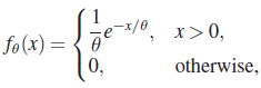
In many problems, especially in location and scale problems, pivots are easily found. For example, in sampling from ![]() is a pivot and so is
is a pivot and so is ![]() . In sampling from (1/σ)f(x/σ) , a scale family,
. In sampling from (1/σ)f(x/σ) , a scale family, ![]() is a pivot and so is X(1)/σ, and in sampling from (1/σ)f((x–θ)/σ), a location-scale family,
is a pivot and so is X(1)/σ, and in sampling from (1/σ)f((x–θ)/σ), a location-scale family, ![]() is a pivot, and so is
is a pivot, and so is ![]() .
.
If the DF Fθ of Xi is continuous, then ![]() and, in case of random sampling, we can take
and, in case of random sampling, we can take

or,

as a pivot. Since ![]() and
and ![]() . It follows that
. It follows that ![]() is a pivot.
is a pivot.
The following result gives a simple sufficient condition for a pivot to yield a confidence interval for a real-valued parameter θ.
Remark 1. The condition that ![]() be solvable will be satisfied if, for example, T is continuous and strictly increasing or decreasing as a function of θ in Θ.
be solvable will be satisfied if, for example, T is continuous and strictly increasing or decreasing as a function of θ in Θ.
Note that in the continuous case (that is, when the DF of T is continuous) we can find a confidence interval with equality on the right side of (1). In the discrete case, however, this is usually not possible.
Remark 2. Relation (1) is valid even when the assumption of monotonicity of T in the theorem is dropped. In that case inversion of the inequalities may yield a set of intervals (random set) S(X) in Θ instead of a confidence interval.
Remark 3. The argument used in Theorem 1 can be extended to cover the multiparameter case, and the method will determine a confidence set for all the parameters of a distribution.
We next consider the method of test inversion and explore the relationship between a test of hypothesis for a parameter θ and confidence interval for θ. Consider the following example.
Conversely, a family of α-level tests for the hypothesis ![]() generates a family of confidence intervals for μ by simply taking, as the confidence interval for μ0, the set of those μ for which one cannot reject
generates a family of confidence intervals for μ by simply taking, as the confidence interval for μ0, the set of those μ for which one cannot reject ![]() .
.
Similarly, we can generate a family of α-level tests from a (1 – α) -level lower (or upper) confidence bound. Suppose that we start with the (1 – α) -level lower confidence bound ![]() for μ. Then, by defining a test φ (Χ) that rejects
for μ. Then, by defining a test φ (Χ) that rejects ![]() if and only if
if and only if ![]() , we get an α-level test for a hypothesis of the form
, we get an α-level test for a hypothesis of the form ![]() .
.
Example 1 is a special case of the duality principle proved in Theorem 2 below. In the following we restrict attention to the case in which the rejection (acceptance) region of the test is the indicator function of a (Borel-measurable) set, that is, we consider only nonrandomized tests (and confidence intervals). For notational convenience we write Η0(θ0) for the hypothesis ![]() and Η1(θ0) for the alternative hypothesis, which may be one- or two-sided.
and Η1(θ0) for the alternative hypothesis, which may be one- or two-sided.
In particular, if X1, X2, … ,Xn is a sample from
then ![]() and for testing
and for testing ![]() against
against ![]() , the UMP acceptance region is of the form
, the UMP acceptance region is of the form

where c(θ0) is the unique solution of

The UMA family of (1 – α) -level confidence sets is of the form
In the case ![]() and
and ![]() .
.
The third method we consider is based on Bayesian analysis where we take into account any prior knowledge that the experimenter has about θ. This is reflected in the specification of the prior distribution π(θ) on Θ. Under this setup the claims of probability of coverage are based not on the distribution of X but on the conditional distribution of θ given ![]() , the posterior distribution of θ.
, the posterior distribution of θ.
Let Θ be the parameter set, and let the observable RV X have PDF (PMF) fθ(x). Suppose that we consider θ as an RV with distribution π(θ) on Θ. Then fθ(x) can be considered as the conditional PDF (PMF) of X, given that the RV θ takes the value θ. Note that we are using the same symbol for the RV θ and the value that it assumes. We can determine the joint distribution of X and θ, the marginal distribution of X, and also the conditional distribution of θ, given ![]() as usual. Thus the joint distribution is given by
as usual. Thus the joint distribution is given by
and the marginal distribution of X by

The conditional distribution of θ, given that x is observed, is given by

Given h(θ | x), it is easy to find functions l(x), u(x) such that
where

depending on whether h is a PDF or a PMF.
One can similarly define one-sided Bayes intervals or (1 – α) -level lower and upper Bayes limits.
Remark 5. We note that, under the Bayesian set-up, we can speak of the probability that θ lies in the interval (l(x), u(x)) with probability 1–α because l and u are computed based on the posterior distribution of θ given x. In order to emphasize this distinction between Bayesian and classical analysis, some authors prefer the term credible sets for Bayesian confidence sets.
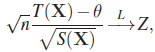
Finally, we consider some large sample methods of constructing confidence intervals. Suppose ![]() . Then
. Then

where Z ~ N(0,1). Suppose further that there is a statistic S(X) such that ![]() . Then, by Slutsky’s theorem
. Then, by Slutsky’s theorem
and we can obtain an (approximate) ![]() -level confidence interval for θ by inverting the inequality
-level confidence interval for θ by inverting the inequality

In particular, we can choose –c1 = c2 = zα/2 to give
as an approximate ![]() -level confidence interval for μ.
-level confidence interval for μ.
Recall that if ![]() is the MLE of θ and the conditions of Theorem 8.7.4 or 8.7.5 are satisfied (caution: See Remark 8.7.4), then
is the MLE of θ and the conditions of Theorem 8.7.4 or 8.7.5 are satisfied (caution: See Remark 8.7.4), then
where

Then we can invert the statement

to give an approximate ![]() -level confidence interval for θ.
-level confidence interval for θ.
Yet another possible procedure has universal applicability and hence can be used for large or small samples. Unfortunately, however, this procedure usually yields confidence intervals that are much too large in length. The method employs the well-known Chebychev inequality (see Section 3.4):
If ![]() is an estimate of θ (not necessarily unbiased) with finite variance σ2(θ), then by Chebychev’s inequality
is an estimate of θ (not necessarily unbiased) with finite variance σ2(θ), then by Chebychev’s inequality

It follows that

is a ![]() -level confidence interval for θ. Under some mild consistency conditions one can replace the normalizing constant
-level confidence interval for θ. Under some mild consistency conditions one can replace the normalizing constant ![]() , which will be some function λ(θ) of θ, by
, which will be some function λ(θ) of θ, by ![]() .
.
Note that the estimator ![]() need not have a limiting normal law.
need not have a limiting normal law.
Actually the confidence interval obtained above can be improved somewhat. We note that

so that

Now
if and only if

This last inequality holds if and only if p lies between the two roots of the quadratic equation

The two roots are

and

It follows that
Note that when n is large

as one should expect in view of the fact that ![]() with probability 1 and
with probability 1 and ![]() estimates
estimates ![]() . Alternatively, we could have used the CLT (or large-sample property of the MLE) to arrive at the same result but with ε replaced by zα/2.
. Alternatively, we could have used the CLT (or large-sample property of the MLE) to arrive at the same result but with ε replaced by zα/2.
In the examples given above we see that, for a given confidence interval ![]() , a wide choice of confidence intervals is available. Clearly, the larger the interval, the better the chance of trapping a true parameter value. Thus the interval
, a wide choice of confidence intervals is available. Clearly, the larger the interval, the better the chance of trapping a true parameter value. Thus the interval ![]() , which ignores the data completely will include the real-valued parameter θ with confidence level 1. However, the larger the confidence interval, the less meaningful it is. Therefore, for a given confidence level 1–α, it is desirable to choose the shortest possible confidence interval. Since the length
, which ignores the data completely will include the real-valued parameter θ with confidence level 1. However, the larger the confidence interval, the less meaningful it is. Therefore, for a given confidence level 1–α, it is desirable to choose the shortest possible confidence interval. Since the length ![]() , in general, is a random variable, one can show that a confidence interval of level 1–α with uniformly minimum length among all such intervals does not exist in most cases. The alternative, to minimize
, in general, is a random variable, one can show that a confidence interval of level 1–α with uniformly minimum length among all such intervals does not exist in most cases. The alternative, to minimize ![]() , is also quite unsatisfactory. In the next section we consider the problem of finding shortest-length confidence interval based on some suitable statistic.
, is also quite unsatisfactory. In the next section we consider the problem of finding shortest-length confidence interval based on some suitable statistic.
PROBLEMS 11.3
- A sample of size 25 from a normal population with variance 81 produced a mean of 81.2. Find a 0.95 level confidence interval for the mean μ.
- Let
 be the mean of a random sample of size n from
  . Find the smallest sample size n such that
  is a 0.90 level confidence interval for μ.
 - Let X1, X2, … ,Xm and Y1, Y2, … ,Yn be independent random samples from
 and
and  , respectively. Find a confidence interval for
  at confidence level 1–α when (a) σ is known and (b) σ is unknown.
 - Two independent samples, each of size 7, from normal populations with common unknown variance σ2 produced sample means 4.8 and 5.4 and sample variances 8.38 and 7.62, respectively. Find a 0.95 level confidence interval for μ1–μ2, the difference between the means of samples 1 and 2.
- In Problem 3 suppose that the first population has variance
 and the second population has variance
  , where both
  , and
, and  are known. Find a
  -level confidence interval for μ1–μ2. What happens if both
  and
and  are unknown and unequal?
 - In Problem 5 find a confidence interval for the ratio
 , both when μ1, μ2 are known and when μ1, μ2 are unknown. What happens if either μ1 or μ2 is unknown but the other is known?
 - Let X1, X2, … ,Xn be a sample from a G(1,ß) distribution. Find a confidence interval for the parameter β with confidence level 1–α.
-
- Use the large-sample properties of the MLE to construct a (1–α) -level confidence interval for the parameter θ in each of the following cases: (i) X1. X2, … ,Xn is a sample from G(1,1/θ) and (ii) X1,X2, … ,Xn is a sample from Ρ(θ).
- In part (a) use Chebychev’s inequality to do the same.
- For a sample of size 1 from the population

find a
 -level confidence interval for θ.
 - Let X1,X2, … ,Xn be a sample from the uniform distribution on N points. Find an upper
 -level confidence bound for N, based on max(X1, X2, … ,Xn).
- In Example 10 find the smallest n such that the length of the
 -level confidence interval
  , provided it is known that
  , where a is a known constant.
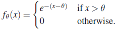
 - Let X and Y be independent RVs with PDFs
 and
and  , respectively. Find a
  -level confidence region for (λ, μ) of the form
  .
.
- Let X1,X2, … ,Xn be a sample from
 , where σ2 is known. Find a UMA
  -level upper confidence bound for μ.
 - Let X1,X2, … ,Xn be a sample from a Poisson distribution with unknown parameter λ. Assuming that λ is a value assumed by a G(α,ß) RV, find a Bayesian confidence interval for λ.
- Let X1,X2, … ,Xn be a sample from a geometric distribution with parameter θ. Assuming that θ has a priori PDF that is given by the density of a B(a,ß) RV, find a Bayesian confidence interval for θ.
- Let X1, X2, … ,Xn be a sample from
 , and suppose that the a priori PDF for μ is U(– 1, 1). Find a Bayesian confidence interval for μ.
11.4 SHORTEST-LENGTH CONFIDENCE INTERVALS
We have already remarked that we can increase the confidence level by simply taking a larger-length confidence interval. Indeed, the worthless interval ![]() , which simply says that θ is a point on the real line, has confidence level 1. In practice, one would like to set the level at a given fixed number
, which simply says that θ is a point on the real line, has confidence level 1. In practice, one would like to set the level at a given fixed number ![]() and, if possible, construct an interval as short in length as possible among all confidence intervals with the same level. Such an interval is desirable since it is more informative. We have already remarked that shortest-length confidence intervals do not always exist. In this section we will investigate the possibility of constructing shortest-length confidence intervals based on simple RVs. The discussion here is based on Guenther [37]. Theorem 11.3.1 is really the key to the following discussion.
and, if possible, construct an interval as short in length as possible among all confidence intervals with the same level. Such an interval is desirable since it is more informative. We have already remarked that shortest-length confidence intervals do not always exist. In this section we will investigate the possibility of constructing shortest-length confidence intervals based on simple RVs. The discussion here is based on Guenther [37]. Theorem 11.3.1 is really the key to the following discussion.
Let X1,X2, … ,Xn be a sample from a PDF fθ(x), and ![]() be a pivot for θ. Also, let
be a pivot for θ. Also, let ![]() be chosen so that
be chosen so that
and suppose that (1) can be rewritten as
For every Tθ, λ1 and λ2 can be chosen in many ways. We would like to choose λ1 and λ2 so that ![]() is minimum. Such an interval is a
is minimum. Such an interval is a ![]() -level shortest-length confidence interval based on Tθ. It may be possible, however, to find another RV
-level shortest-length confidence interval based on Tθ. It may be possible, however, to find another RV ![]() that may yield an even shorter interval. Therefore we are not asserting that the procedure, if it succeeds, will lead to a
that may yield an even shorter interval. Therefore we are not asserting that the procedure, if it succeeds, will lead to a ![]() -level confidence interval that has shortest length among all intervals of this level. For Tθ we use the simplest RV that is a function of a sufficient statistic and θ.
-level confidence interval that has shortest length among all intervals of this level. For Tθ we use the simplest RV that is a function of a sufficient statistic and θ.
Remark 1. An alternative to minimizing the length of the confidence interval is to minimize the expected length ![]() . Unfortunately, this also is quite unsatisfactory since, in general, there does not exist a member of the class of all
. Unfortunately, this also is quite unsatisfactory since, in general, there does not exist a member of the class of all ![]() -level confidence intervals that minimizes
-level confidence intervals that minimizes ![]() for all θ. The procedures applied in finding the shortest-length confidence interval based on a pivot are also applicable in finding an interval that minimizes the expected length. We remark here that the restriction to unbiased confidence intervals is natural if we wish to minimize
for all θ. The procedures applied in finding the shortest-length confidence interval based on a pivot are also applicable in finding an interval that minimizes the expected length. We remark here that the restriction to unbiased confidence intervals is natural if we wish to minimize ![]() . See Section 11.5 for definitions and further details.
. See Section 11.5 for definitions and further details.
The length of this interval is ![]() . In this case we can plan our experiment to give a prescribed confidence level and a prescribed length for the interval. To have level
. In this case we can plan our experiment to give a prescribed confidence level and a prescribed length for the interval. To have level ![]() and length
and length ![]() , we choose the smallest n such that
, we choose the smallest n such that

This can also be interpreted as follows. If we estimate μ by ![]() , taking a sample of size
, taking a sample of size ![]() , we are 100
, we are 100 ![]() percent confident that the error in our estimate is at most d.
percent confident that the error in our estimate is at most d.
It follows that the minimum occurs at ![]() (the other solution,
(the other solution, ![]() , is not admissible). The shortest-length confidence interval based on Tμ is the equal-tails interval,
, is not admissible). The shortest-length confidence interval based on Tμ is the equal-tails interval,

The length of this interval is ![]() , which, being random, may be arbitrarily large. Note that the same confidence interval minimizes the expected length of the interval, namely,
, which, being random, may be arbitrarily large. Note that the same confidence interval minimizes the expected length of the interval, namely, ![]() , where cn is a constant determined from
, where cn is a constant determined from ![]() and the minimum expected length is
and the minimum expected length is ![]() .
.
Numerical results giving values of a and b to four significant places of decimals are available (see Tate and Klett [112]). In practice, the simpler equal-tails interval,

may be used.
If μ is unknown, we use
as a pivot. ![]() has a χ2(n–1) distribution. Proceeding as above, we can show that the shortest-length confidence interval based on
has a χ2(n–1) distribution. Proceeding as above, we can show that the shortest-length confidence interval based on ![]() is
is ![]() ; here a and b are a solution of
; here a and b are a solution of
and
where fn—1 is the PDF of a ![]() RV. Numerical solutions due to Tate and Klett [112]may be used, but, in practice, the simpler equal-tails confidence interval,
RV. Numerical solutions due to Tate and Klett [112]may be used, but, in practice, the simpler equal-tails confidence interval,

is employed.
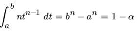
Using Tθ as pivot, we see that the confidence interval is (X(n)/b, X(n)/a) with length ![]() . We minimize L subject to
. We minimize L subject to
Now
and
so that the minimum occurs at ![]() . The shortest interval is therefore
. The shortest interval is therefore ![]() .
.
Note that

which is minimized subject to
where ![]() and
and ![]() . The expected length of the interval that minimizes EL is
. The expected length of the interval that minimizes EL is ![]() , which is also the expected length of the shortest confidence interval based on X(n).
, which is also the expected length of the shortest confidence interval based on X(n).
Note that the length of the interval ![]() goes to 0 as
goes to 0 as ![]() .
.
For some results on asymptotically shortest-length confidence intervals, we refer the reader to Wilks [118, pp. 374–376].
PROBLEMS 11.4
- Let X1,X2, … ,Xn be a sample from

Find the shortest-length confidence interval for θ at level
 based on a sufficient statistic for θ.
 - Let X1,X2, … ,Xn be a sample from G(1,θ). Find the shortest-length confidence interval for θ at level
 , based on a sufficient statistic for θ.
 - In Problem 11.3.9 how will you find the shortest-length confidence interval for θ at level
 , based on the statistic X/θ?
 - Let T (Χ, θ) be a pivot of the form
 . Show how one can construct a confidence interval for θ with fixed width d and maximum possible confidence coefficient. In particular, construct a confidence interval that has fixed width d and maximum possible confidence coefficient for the mean μ of a normal population with variance 1. Find the smallest size n for which this confidence interval has a confidence coefficient
  . Repeat the above in sampling from an exponential PDF
(Desu [21])
- Let X1, X2, … ,Xn be a random sample from

Find the shortest-length (1–α) -level confidence interval for θ, based on the sufficient statistic
 .
. - In Example 4, let
 . Find a (1–α) -level confidence interval for θ of the form (R, R/c). Compare the expected length of this interval to the one computed in Example 4.
 - Let X1, X2, … ,Xn be a random sample from a Pareto PDF
 , and = 0 for
  . Show that the shortest-length confidence interval for θ based on X(1) is (X(1)α1/n, X(1)). (Use θ/X(1) as a pivot.)
 - Let X1, X2, … ,Xn be a sample from PDF
 and = 0 otherwise. Let
  . Using
  as a pivot for estimating
  , show that the shortest-length confidence interval is of the form (R, R/c), where c is determined from the level as a solution of
cn—1{(n – 1)c – n} + a = 0 (Ferentinos [27]).
, show that the shortest-length confidence interval is of the form (R, R/c), where c is determined from the level as a solution of
cn—1{(n – 1)c – n} + a = 0 (Ferentinos [27]).
11.5 UNBIASED AND EQUIVARIANT CONFIDENCE INTERVALS
In Section 11.3 we studied test inversion as one of the methods of constructing confidence intervals. We showed that UMP tests lead to UMA confidence intervals. In Chapter 9 we saw that UMP tests generally do not exist. In such situations we either restrict consideration to smaller subclasses of tests by requiring that the test functions have some desirable properties, or we restrict the class of alternatives to those near the null parameter values.
In this section will follow a similar approach in constructing confidence intervals.
Remark 1. Definition 1 says that a family S(X) of confidence sets for a parameter θ is unbiased at level ![]() if the probability of true coverage is at least
if the probability of true coverage is at least ![]() and that of false coverage is at most
and that of false coverage is at most ![]() . In other words, S(X) traps a true parameter value more often than it does a false one.
. In other words, S(X) traps a true parameter value more often than it does a false one.
We next show that S(X) is UMA. Let S*(x) be any other unbiased ![]() -level family of confidence sets, and write
-level family of confidence sets, and write ![]() contains θ}. Then
contains θ}. Then ![]() , and it follows that Α*(θ) is the acceptance region of an unbiased size α test. Hence
, and it follows that Α*(θ) is the acceptance region of an unbiased size α test. Hence

The inequality follows since Α(θ) is the acceptance region of a UMP unbiased test. This completes the proof.
If the measure of precision of a confidence interval is its expected length, one is naturally led to a consideration of unbiased confidence intervals. Pratt [81]has shown that the expected length of a confidence interval is the average of false coverage probabilities.
Remark 2. If S(X) is a family of UMAU ![]() -level confidence intervals, the expected length of S(X) is minimal. This follows since the left-hand side of (3) is the expected length, if θ is the true value, of S(X) and Ρθ{S(X) contains θ'} is minimal [because S(X) is UMAU], by Theorem 1, with respect to all families of
-level confidence intervals, the expected length of S(X) is minimal. This follows since the left-hand side of (3) is the expected length, if θ is the true value, of S(X) and Ρθ{S(X) contains θ'} is minimal [because S(X) is UMAU], by Theorem 1, with respect to all families of ![]() unbiased confidence intervals uniformly in
unbiased confidence intervals uniformly in ![]() .
.
Since a reasonably complete discussion of UMP unbiased tests (see Section 9.5) is beyond the scope of this text, the following procedure for determining unbiased confidence intervals is sometimes quite useful (see Guenther [38]). Let X1,X2, … ,Xn be a sample from an absolutely continuous DF with PDF fθ (x) and suppose that we seek an unbiased confidence interval for θ. Following the discussion in Section 11.4, suppose that
is a pivot, and suppose that the statement
can be converted to
In order for ![]() to be unbiased, we must have
to be unbiased, we must have
and
If Ρ(θ, θ') depends only on a function γ of θ, θ', we may write

and it follows that Ρ(γ) has a maximum at ![]() .
.
Finally, let us briefly investigate how invariance considerations apply to confidence estimation. Let ![]() . Let
. Let ![]() be a group of transformations on
be a group of transformations on ![]() which leaves
which leaves ![]() invariant. Let S(X) be a
invariant. Let S(X) be a ![]() -level confidence set for θ.
-level confidence set for θ.
The most useful method of constructing invariant confidence intervals is test inversion. Inverting the acceptance region of invariant tests often leads to equivariant confidence intervals under certain conditions. Recall that a group ![]() of transformations leaves a hypothesis testing problem invariant if
of transformations leaves a hypothesis testing problem invariant if ![]() leaves both Θ0 and Θ1 invariant. For each
leaves both Θ0 and Θ1 invariant. For each ![]() , we have a different group of transformations,
, we have a different group of transformations, ![]() , which leaves the problem of testing
, which leaves the problem of testing ![]() invariant. The equivariant confidence interval, on the other hand, must be equivariant with respect to
invariant. The equivariant confidence interval, on the other hand, must be equivariant with respect to ![]() , which is a much larger group since
, which is a much larger group since ![]() for all θ0. The relationship between an equivariant confidence set and invariant tests is more complicated when the family
for all θ0. The relationship between an equivariant confidence set and invariant tests is more complicated when the family ![]() has a nuisance parameter τ.
has a nuisance parameter τ.
Under certain conditions there is a relationship between equivariant confidence sets and associated invariant tests. Rather than pursue this relationship, we refer the reader to Ferguson [28, p. 262]; it is generally easy to check that (10) holds for a given confidence interval S to show that S is invariant. The following example illustrates this point.
PROBLEMS 11.5
- Let X1, X2, … ,Xn be a sample from U(0,θ). Show that the unbiased confidence intervals for θ based on the pivot max Xi/θ coincides with the shortest-length confidence interval based on the same pivot.
- Let X1,X2, … ,Xn be a sample from G(1,θ). Find the unbiased confidence interval for θ based on the pivot 2
 .
.
- Let X1, X2, … ,Xn be a sample from PDF
Find the unbiased confidence interval based on the pivot 2n[min Xi–θ].
- Let X1,X2, … ,Xn be iid
 (μ,σ2) RVs where both μ and σ2 are unknown. Using the pivot
  show that the shortest-length unbiased (1–α) -level confidence interval for μ is the equal-tails interval
  .
. - Let X1, X2, … ,Xn be iid with PDF
 , and
, and  otherwise. Find the shortest-length
  -level unbiased confidence interval for θ based on the pivot θ/X(1) .
- Let X1,X2, … ,Xn be a random sample from a location family
 . Show that a confidence interval of the form
  where T(x) is an equivariant estimate under location group is an equivariant confidence interval.
 - Let X1,X2, … ,Xn be iid RVs with common scale PDF
 . Consider the scale group
  . If T(x) is an equivariant estimate of σ, show that a confidence interval of the form
is equivariant.
- Let X1,X2, … ,Xn be iid RVs with PDF
 and,
and,  , otherwise. For testing
  against
  , consider the (UMP) test
Is the acceptance region of this α-level test an equivariant (1 – α) -level confidence interval (lower bound) for θ with respect to the location group?
Yes.
11.6 RESAMPLING: BOOTSTRAP METHOD
In many applications of statistical inference the investigator has a random sample from a population distribution DF F which may or may not be completely specified. Indeed the empirical data may not even fit any known distribution. The inference is typically based on some statistic such as ![]() , S2, a percentile or some much more complicated statistic such as sample correlation coefficient or odds ratio. For this purpose we need to know the distribution of the statistic being used and/or its moments. Except for the simple situations such as those described in Chapter 6 this is not easy. And even if we are able to get a handle on it, it may be inconvenient to deal with it. Often, when the sample is large enough, one can resort to asymptotic approximations considered in Chapter 7. Alternatively, one can use computer-intensive techniques which have become quite popular in the last 25 years due to the availability of fast home or office laptops and desktops.
, S2, a percentile or some much more complicated statistic such as sample correlation coefficient or odds ratio. For this purpose we need to know the distribution of the statistic being used and/or its moments. Except for the simple situations such as those described in Chapter 6 this is not easy. And even if we are able to get a handle on it, it may be inconvenient to deal with it. Often, when the sample is large enough, one can resort to asymptotic approximations considered in Chapter 7. Alternatively, one can use computer-intensive techniques which have become quite popular in the last 25 years due to the availability of fast home or office laptops and desktops.
Suppose x1, x2, … ,xn is a random sample from a distribution F with unknown parameter θ(F), and let ![]() be an estimate of θ(F). What is the bias of
be an estimate of θ(F). What is the bias of ![]() and its SE? Resampling refers to sampling from x1, x2, … ,xn and using these samples to estimate the statistical properties of
and its SE? Resampling refers to sampling from x1, x2, … ,xn and using these samples to estimate the statistical properties of ![]() . Jackknife is one such method where one uses subsets of the sample by excluding one or more observations at a time. For each of these subsamples an estimate θj of θ is computed, and these estimates are then used to investigate the statistical properties of
. Jackknife is one such method where one uses subsets of the sample by excluding one or more observations at a time. For each of these subsamples an estimate θj of θ is computed, and these estimates are then used to investigate the statistical properties of ![]() .
.
The most commonly used resampling method is the bootstrap , introduced by Efron [22], where one draws random samples of size n, with replacement, from x1, x2, … ,xn. This allows us to generate a large number of bootstrap samples and hence bootstrap estimates ![]() of θ. This bootstrap distribution of
of θ. This bootstrap distribution of ![]() is then used to study the statistical properties of
is then used to study the statistical properties of ![]() .
.
Let ![]() , be iid RVs with common DF
, be iid RVs with common DF ![]() , the empirical DF corresponding to the sample x1, x2, … ,xn. Then
, the empirical DF corresponding to the sample x1, x2, … ,xn. Then ![]() is called a bootstrap sample . Let θ be the parameter of interest associated with DF F and suppose we have chosen
is called a bootstrap sample . Let θ be the parameter of interest associated with DF F and suppose we have chosen ![]() to be an estimate of θ based on the sample x1, x2, … ,xn. For each bootstrap sample let
to be an estimate of θ based on the sample x1, x2, … ,xn. For each bootstrap sample let ![]() , be the corresponding bootstrap estimate of θ. We can now study the statistical properties of
, be the corresponding bootstrap estimate of θ. We can now study the statistical properties of ![]() based on the distribution of the
based on the distribution of the ![]() , values. Let
, values. Let ![]() Then the variance of
Then the variance of ![]() is estimated by the bootstrap variance.
is estimated by the bootstrap variance.
Similarly the bias of ![]() , is estimated by
, is estimated by
Arranging the values of ![]() , in increasing order of magnitude and then excluding 100α/2 percent smallest and largest values we get a (1–α) -level confidence interval for θ. This is the so-called percentile confidence interval. One can also use this confidence interval to test hypotheses concerning θ.
, in increasing order of magnitude and then excluding 100α/2 percent smallest and largest values we get a (1–α) -level confidence interval for θ. This is the so-called percentile confidence interval. One can also use this confidence interval to test hypotheses concerning θ.
We took 1000 random samples, with replacement, of size 20 each from this sample with the following distribution of ![]() .
.
| Interval | Frequency |
| 0.49–0.56 | 6 |
| 0.53–0.57 | 29 |
| 0.57–0.61 | 109 |
| 0.61–0.65 | 200 |
| 0.65–0.69 | 234 |
| 0.69–0.73 | 229 |
| 0.73–0.77 | 123 |
| 0.77–0.81 | 59 |
| 0.81–0.85 | 10 |
| 0.85–0.89 | 2 |
The bootstrap estimate of θ is ![]() and that of the variance is 0.061. By excluding the smallest and the largest twenty-five vales of
and that of the variance is 0.061. By excluding the smallest and the largest twenty-five vales of ![]() a 95 percent confidence interval for θ is given by (0.564, 0.793). (We note that
a 95 percent confidence interval for θ is given by (0.564, 0.793). (We note that ![]() and
and ![]() so the
so the ![]() .)
.)
Figure 1 show the frequency distribution of the bootstrap statistic ![]() .
.

It is natural to ask how well does the distribution of the bootstrap statistic ![]() approximate the distribution of
approximate the distribution of ![]() ? The bootstrap approximation is often better when applied to the appropriately centered
? The bootstrap approximation is often better when applied to the appropriately centered ![]() . Thus to estimate population mean θ bootstrap is applied to the centered sample mean
. Thus to estimate population mean θ bootstrap is applied to the centered sample mean ![]() . The corresponding bootstrapped version will then be
. The corresponding bootstrapped version will then be ![]() , where
, where ![]() is the sample mean of the bth bootstrap sample. Similarly if
is the sample mean of the bth bootstrap sample. Similarly if ![]() then the bootstrap approximation will be applied to the centered sample median
then the bootstrap approximation will be applied to the centered sample median ![]() . The bootstrap version will be then be
. The bootstrap version will be then be ![]() . Similarly , in estimation of the distribution of sample variance S2, the bootstrap version will be applied to the ratio S2/σ2, where σ2 is the variance of the DF F.
. Similarly , in estimation of the distribution of sample variance S2, the bootstrap version will be applied to the ratio S2/σ2, where σ2 is the variance of the DF F.
We have already considered the percentile method of constructing confidence intervals. Let us denote the αth percentile of the distribution of ![]() ,by Bα. Suppose that the sampling distribution of
,by Bα. Suppose that the sampling distribution of ![]() is approximated by the bootstrap distribution of
is approximated by the bootstrap distribution of ![]() . Then the probability that
. Then the probability that ![]() is covered by the interval
is covered by the interval ![]() is approximately
is approximately ![]() . This is called a
. This is called a ![]() -level centered bootstrap percentile confidence interval for θ.
-level centered bootstrap percentile confidence interval for θ.
Recall that in sampling from a normal distribution when both mean and the variance are unknown, a ![]() -level confidence interval for the mean θ is based on t-statistic and is given by
-level confidence interval for the mean θ is based on t-statistic and is given by ![]() . For nonnormal distributions the bootstrap analog of the Student’s t-statistic is the statistic
. For nonnormal distributions the bootstrap analog of the Student’s t-statistic is the statistic ![]() . The bootstrap version is the statistic
. The bootstrap version is the statistic ![]() , where SEb is the SE computed from the bootstrap sample distribution. A
, where SEb is the SE computed from the bootstrap sample distribution. A ![]() -level confidence interval is now easily constructed.
-level confidence interval is now easily constructed.
In our discussion above we have assumed that F(θ) is completely unspecified. What if we know F except for the parameter θ? In that case we take bootstrap samples from the distribution ![]() .
.
We refer the reader to Efron and Tibshirani [23]for further details.
PROBLEMS 11.6
-
- Show that there are
 distinct bootstrap samples of size n. [Hint: Problem 1.4.17.]
 - What is the probability that a bootstrap sample is identical to the original samples?
- What is the most likely bootstrap sample to be drawn?
- What is the mean number of times that xi appears in the bootstrap samples?
- Show that there are
- Let x1, x2,…xn be a random sample. Then
 is an estimate of the unknown mean μ. Consider the leave-one-out Jackknife sample. Let
  be the mean of the remaining (n – 1) observations when xi is excluded:
- Show that
 .
. - Now suppose we need to estimate a parameter θ and choose
 to be an estimate from the sample. Imitating the Jackknife procedure for estimating μ we note that
  . What is the Jackknife estimate of θ? What is the Jackknife estimate of the bias of
  and its variance?
- Show that
- Let x1, x2,… ,xn be a random sample from
 and suppose that
  is an estimate of θ. Let
  be a bootstrap sample from
  . Show that both
  and
and  have the same
  distribution.
 - Consider the data set

Let
 , be a bootstrap sample from this data set:
- Find the probability that the bootstrap mean equals 2.
- Find the probability that the maximum value of the bootstrap mean is 9.
- Find the probability that the bootstrap sample mean is 4.