Search in book...
Toggle Font Controls
Create new playlist

Name your new playlist

Playlist description (optional)
Sign In

Email address

Password

Forgot Password?

or

Continue with Facebook

Continue with Google
Sign Up

Full Name

Email address

Confirm Email Address

Password

or

Continue with Facebook

Continue with Google

9
NEYMAN–PEARSON THEORY OF TESTING OF HYPOTHESES

9.1 INTRODUCTION

Let X₁, X₂, …, X_n be a random sample from a population distribution F_θ, , where the functional form of F_θ is known except, perhaps, for the parameter θ. Thus, for example, the X_i’s may be a random sample from (θ,1), where is not known. In many practical problems the experimenter is interested in testing the validity of an assertion about the unknown parameter θ. For example, in a coin-tossing experiment it is of interest to test, in some sense, whether the (unknown) probability of heads p equals a given number , Similarly, it is of interest to check the claim of a car manufacturer about the average mileage per gallon of gasoline achieved by a particular model. A problem of this type is usually referred to as a problem of testing of hypotheses and is the subject of discussion in this chapter. We will develop the fundamentals of Neyman–Pearson theory. In Section 9.2 we introduce the various concepts involved. In Section 9.3 the fundamental Neyman–Pearson lemma is proved, and Sections 9.4 and 9.5 deal with some basic results in the testing of composite hypotheses. Section 9.6 deals with locally optimal tests.

9.2 SOME FUNDAMENTAL NOTIONS OF HYPOTHESES TESTING

In Chapter 8 we discussed the problem of point estimation in sampling from a population whose distribution is known except for a finite number of unknown parameters. Here we consider another important problem in statistical inference, the testing of statistical hypotheses. We begin by considering the following examples.

To fix ideas, let us define formally the concepts involved. As usual, and let . It will be assumed that the functional form of F_θ is known except for the parameter θ. Also, we assume that Θ contains at least two points.

Usually the null hypothesis is chosen to correspond to the smaller or simpler subset Θ₀ of Θ and is a statement of “no difference,” whereas the alternative represents change.

The problem of testing of hypotheses may be described as follows: Given the sample point , find a decision rule (function) that will lead to a decision to reject or fail to reject the null hypothesis. In other words, partition the sample space into two disjoint sets C and C^c such that, if x ∈ C, we reject H₀, and if x ∈ C^c, we fail to reject H₀. In the following we will write accept H₀ when we fail to reject H₀. We emphasize that when the sample point x ∈C^c and we fail to reject H₀, it does not mean that H₀ gets our stamp of approval. It simply means that the sample does not have enough evidence against H₀.

There are two types of errors that can be made if one uses such a procedure. One may reject H₀ when in fact it is true, called a type I error, or accept H₀ when it is false, called a type II error,

If C is the critical region of a rule, , is a probability of type I error, and , is a probability of type II error. Ideally, one would like to find a critical region for which both these probabilities are 0. This will be the case if we can find a subset such that for every and for every . Unfortunately, situations such as this do not arise in practice, although they are conceivable. For example, let under H₀ and under H₁. Usually, if a critical region is such that the probability of type I error is 0, it will be of the form “do not reject H₀” and the probability of type II error will then be 1.

The procedure used in practice is to limit the probability of type I error to some pre-assigned level α (usually 0.01 or 0.05) that is small and to minimize the probability of type II error. To restate our problem in terms of this requirement, let us formulate these notions.

Some simple examples of test functions are for all for all , or , for all . In fact, Definition 4 includes Definition 3 in the sense that, whenever φ is the indicator function of some Borel subset A of , A is called the critical region (of the test φ).

The following interpretation may be given to all tests φ satisfying for all . To every we assign a number , which is the probability of rejecting H₀ that , if x is observed. The restriction then says that, if H₀ were true, φ rejects it with a probability ≤ α. We will call such a test a randomized test function. If will be called a nonrandomized test. If , we reject H₀ with probability 1; and if , this probability is 0. Needless to say, .

We next turn our attention to the type II error.

In view of Definitions 5 and 6 the problem of testing of hypotheses may now be reformulated. Let . Also, let be given. Given a sample point x, find a test φ(x) such that , and β_φ(θ) is a maximum for .

Note that if φ₁, φ₂ are two tests and λ is a real number, , then is also a test function, and it follows that the class of all test functions Φ_α is convex.

Example 5.

Let X₁, X₂, …, X_n be iid (μ,1)RVs, where μ is unknown but it is known that , . Let . Both H₀ and H₁ are simple hypotheses. Intuitively, one would accept H₀ if the sample mean is “closer” to μ₀ than to μ₁; that is to say, one would reject H₀ if , and accept H₀ otherwise. The constant k is determined from the level requirements. Note that, under H_0, , and, under H_1, . Given , we have

so that . The test, therefore, is (Fig. 1)

Fig. 1 Rejection region of H₀ in Example 5.

Here is known as a test statistic, and the test φ is nonrandomized with critical region . Note that in this case the continuity of X (that is, the absolute continuity of the DF of X) allows us to achieve any size α, .

The power of the test at μ₁ is given by

where Z ~ (0,1). In particular, since . The probability of type II error is given by

Figure 2 gives a graph of the power function β_φ(μ) of φ for when , and .

Fig. 2 Power function of φ in Example 5.

Example 6.

Let X₁,X₂,X₃,X₄,X₅, be a sample from b(1,p), where p is unknown and . Consider the simple null hypothesis , that is, under. . Then . A reasonable procedure would be to compute the average number of 1's, namely, , and to accept , where c is to be determined. Let . Then we would like to choose c such that the size of our test is α, that is,

(6)

wher . Now under H₀, so that the PMF of is given in the following table.


0	–2.5	0.03125
1	–1.5	0.15625
2	–0.5	0.31250
3	0.5	0.31250
4	1.5	0.15625
5	2.5	0.03125

Note that we cannot choose any k to satisfy (6) exactly. It is clear that we have to reject H₀ when , that is, when we observe or 5. The resulting size if we use this test is . A second procedure would be to reject H₀ if , in which case the resulting size is , which is considerably larger than 0.10. A third alternative, if we insist on achieving , is to randomize on the boundary. Instead of accepting or rejecting H₀ with probability 1 when or 4, we reject H₀ with probability γ where

Thus

A randomized test of size is therefore given by

The power of this test is

where and can be computed for any value of p. Figure 3 gives a graph of β_φ(p).

Fig. 3 Power function of φ in Example 6.

We conclude this section with the following remarks.

Remark 1. The problem of testing of hypotheses may be considered as a special case of the general decision problem described in Section 8.8. Let , where a₀ represents the decision to accept and a₁ represents the decision to reject H₀. A decision function δ is a mapping of into . Let us introduce the following loss functions:

and

Then the minimization of E_θL₂(θ, δ(X)) subject to is the hypotheses testing problem discussed above. We have

and

Remark 2. In Example 6 we saw that the chosen size α is often unattainable. The choice of a specific value of α is completely arbitrary and is determined by nonstatistical considerations such as the possible consequences of rejecting H₀ falsely, and the economic and practical implications of the decision to reject H₀. An alternative, and somewhat subjective, approach wherever possible is to report the so-called P-value of the observed test statistic. This is the smallest level ∝ at which the observed sample statistic is significant. In Example 6, let is observed, then . By symmetry, if we reject H₀ for we should do so also for so the probability of interest is which is the P-value. If is observed and we decide to reject H₀, then we would do so also for because is more extreme than . By symmetry considerations

This discussion motivates Definition 9 below. Suppose the appropriate critical region for testing H₀ against H₁ is one-sided. That is, suppose C is either of the form or , where T is the test statistic.

If α is given, then we reject H₀ if and do not reject H₀ if . In the two-sided case when the critical region is of the form , the one-sided P-value is doubled to obtain the P-value. If the distribution of T is not symmetric then the P-value is not well-defined in the two-sided case although many authors recommend doubling the one-sided P-value.

PROBLEMS 9.2

A sample of size 1 is taken from a population distribution P(λ). To test against , consider the nonrandomized test if . Find the probabilities of type I and type II errors and the power of the test against . If it is required to achieve a size equal to 0.05, how should one modify the test φ?
0.019, 0.857.
Let X₁, X₂, …,X_n be a sample from a population with finite mean μ and finite variance σ². Suppose that μ is not known, but σ is known, and it is required to test against . Let n be sufficiently large so that the central limit theorem holds, and consider the test

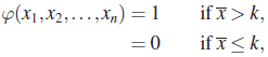
where . Find k such that the test has (approximately) size α. What is the power of this test at ? If the probabilities of type I and type II errors are fixed at α and β, respectively, find the smallest sample size needed.

.
In Problem 2, if σ is not known, find k such that the test φ has size α.
Let X₁,X₂, …,X_n be a sample from (μ, 1) For testing against consider the test function

Show that the power function of φ is a nondecreasing function of μ. What is the size of the test?
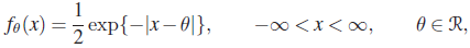
A sample of size 1 is taken from an exponential PDF with parameter θ, that is, . Totest , against , the test to be used is the nonrandomized test

Find the size of the test. What is the power function?
Let X₁, X₂, …,X_n be a sample from (0, σ²). To test against , it is suggested that the test

be used. How will you find c₁ and c₂ such that the size of φ is a preassigned number ? What is the power function of this test?
An urn contains 10 marbles, of which M are white and 10–M are black. To test that against the alternative hypothesis that , one draws 3 marbles from the urn without replacement. The null hypothesis is rejected if the sample contains 2 or 3 white marbles; otherwise it is accepted. Find the size of the test and its power.

9.3 NEYMAN–PEARSON LEMMA

In this section we prove the fundamental lemma due to Neyman and Pearson [76], which gives a general method for finding a best (most powerful) test of a simple hypothesis against a simple alternative. Let , where , be a family of possible distributions of X. Also, f_θ represents the PDF of X if X is a continuous type rv, and the PMF of X if X is of the discrete type. Let us write and for convenience.

Theorem 1 (The Neyman–Pearson Fundamental Lemma).

Any test φ of the form
(1)
for some and , is most powerful of its size for testing against . If , the test
(2)
is most powerful of size 0 for testing H₀ against H₁.
Given , there exists a test of form (1) or (2) with (a constant), for which .

Proof. Let φ be a test satisfying (1), and φ* be any test with . In the continuous case

For any , so that the integrand is . For , so that the integrand is again . It follows that

which implies

since

If , any test φ* of size 0 must vanish on the set . We have

The proof for the discrete case requires the usual change of integral by a sum throughout.

To prove (b) we need to restrict ourselves to the case where , since the MP size 0 test is given by (2). Let , and let us compute the size of a test of form (1). We have

Since , we may rewrite as

(3)

Given , we wish to find k and γ such that , that is,

(4)

Note that

is a DF so that it is a nondecreasing and right continuous function of k. If there exists a k₀ such that

we choose and . Otherwise there exists a k₀ such that

(5)

that is, there is a jump at k₀ (see Fig. 1). In this case we choose k = k₀ and

Fig. 1

(6)

Since γ given by (6) satisfies (4), and , the proof is complete.

Remark 1. It is possible to show (see Problem 6) that the test given by (1) or (2) is unique (except on a null set), that is, if φ is an MP test of size α of H₀ against H₁, it must have form (1) or (2), except perhaps for a set A with .

Remark 2. An analysis of proof of part (a) of Theorem 1 shows that test (1) is MP even if f₁ and f₀ are not necessarily densities.

Remark 3. If the family admits a sufficient statistic, one can restrict attention to tests based on the sufficient statistic, that is, to tests that are functions of the sufficient statistic. If φ is a test function and T is a sufficient statistic, is itself a test function, , and

so that φ and have the same power function.

Example 3.

Let X₁, X₂, …, X_n be iid b(1, p) RVs, and let . The MP size α test of H₀ against H₁ is of the form

where k and γ are determined from

Now

and since is an increasing function of It follows that if and only if , where k₁ is some constant. Thus the MP size α test is of the form

Also, k₁ and γ are determined from

Note that the MP size α test is independent of p₁ as long as p₁ > p₀, that is, it remains an MP size α test against any p > p₀ and is therefore a UMP test of p = p₀ against p > p₀.

In particular, let . Then the MP test is given by

where k and γ are determined from

It follows that and . Thus the MP size test is to reject in favor of and reject with probability 0.122 if .

It is simply a matter of reversing inequalities to see that the MP size α test of against is given by

where γ and k are determined from .

We note that is minimal sufficient for p so that, in view of Remark 3, we could have considered tests based only on T. Since ,

so that an MP Test is of the same form as above but the computation is somewhat simpler.

We remark that in both cases the MP test is quite intuitive. We would tend to accept the larger probability if a larger number of “successes” showed up, and the smaller probability if a smaller number of “successes” were observed. See, however, Example 2.

PROBLEMS 9.3

A sample of size 1 is taken from PDF

Find an MP test of against .
Find the Neyman–Pearson size α test of against based on a sample of size 1 from the PDF
Find the Neyman–Pearson size α test of against based on a sample of size 1 from
Find an MP size α test of , where , against whhere , based on a sample of size 1.
For the PDF , find an MP size α test of against , based on a sample of size n.
If φ* is an MP size α test of against show that it has to be either of form (1) or form (2) (except for a set of x that has probability 0 under H₀ and H₁).
Let φ* be an MP size α test of H₀ against H₁, and let k(α) denote the value of k in (1). Show that if , then .
For the family of Neyman–Pearson tests show that the larger the α the smaller the .
Let be the power of an MP size α test, where . Show that unless .
Let α be a real number, , and be an MP size α test of H₀ against H₁. Also, let . Show that is an MP test for testing H₁ against H₀ at level .
Let X₁, X₂, …,X_n be a random sample from PDF

Find an MP test of against .
Let X be an observation in (0,1). Find an MP size α test of if , and , against . Find the power of your test.
In each of the following cases of simple versus simple hypotheses , draw a graph of the ratio and find the form of the Neyman–Pearson test:
Let X₁, X₂,…, X_n be a random sample with common PDF

Find a size α MP test for testing versus .
Let , where
1. Find the form of the MP test of its size.
2. Find the size and the power of your test for various values of the cutoff point.
3. Consider now a random sample of size n from f₀ under H₀ or f₁ under H₁. Find the form of the MP test of its size.

9.4 FAMILIES WITH MONOTONE LIKELIHOOD RATIO

In this section we consider the problem of testing one-sided hypotheses on a single real-valued parameter. Let be a family of PDFs (PMFs), , and suppose that we wish to test against the alternatives or its dual, , against . In general, it is not possible to find a UMP test for this problem. The MP test of , say, against the alternative depends on θ₁ and cannot be UMP. Here we consider a special class of distributions that is large enough to include the one-parameter exponential family, for which a UMP test of a one-sided hypothesis exists.

It is also possible to define families of densities with nonincreasing MLR in T(x), but such families can be treated by symmetry.

Remark 1. The nondecreasingness of Q(θ) can be obtained by a reparametrization, putting , if necessary.

Theorem 1 includes normal, binomial, Poisson, gamma (one parameter fixed), beta (one parameter fixed), and so on. In Example 1 we have already seen that U[0, θ], which is not an exponential family, has an MLR.

Theorem 2

Let , where {f_θ} has an MLR in T(x). For testing against , any test of the form

(2)

has a nondecreasing power function and is UMP of its size (provided that the size is not 0).

Moreover, for every and every , there exists a , and such that the test described in (2) is the UMP size α test of H₀ against H₁.

Proof. Let . By the fundamental lemma any test of the form

(3)

where is MP of its size for testing against , provided that and if , the test

(4)

is MP of size 0. Since f_θ has an MLR in T, it follows that any test of form (2) is also of form (3), provided that , that is, provided that its size is > 0. The trivial test has size α and power α, so that the power of any test (2) is at least α, that is,

It follows that, if and , then , as asserted.

Let and , as above. We know that (2) is an MP test of its size , for testing against , provided that . Since the power function of φ is nondecreasing,

(5)

Since, however, φ does not depend on θ₂ (it depends only on constants k and γ), it follows that φ is the UMP size α₀ test for testing against . Thus φ is UMP among the class of tests φ″ for which

(6)

Now the class of tests satisfying (5) is contained in the class of tests satisfying (6) [there are more restrictions in (5)]. It follows that φ, which is UMP in the larger class satisfying (6), must also be UMP in the smaller class satisfying (5). Thus, provided that is the UMP size α₀ test for against .

We ask the reader to complete the proof of the final part of the theorem, using the fundamental lemma.

Remark 2. By interchanging inequalities throughout in Theorem 2, we see that this theorem also provides a solution of the dual problem against .

Remark 3. We caution the reader that UMP tests for testing and for the one-parameter exponential family do not exist. An example will suffice.

PROBLEMS 9.4

For the following families of PMFs (PDFs) , find a UMP size α test of against , based on a sample of n observations.
1. .
2. .
3. .
4. .
5. .
6. .
Let X₁, X₂, …X_n be sample of size n from the PMF
1. Show that test
  
  is UMP size α for testing against .
2. Show that
  
  is a UMP size α test of against .
Let X₁, X₂, …,X_n be a sample of size n from . Show that the test

is UMP size α for testing against and that the test

is UMP size α for against .
Does the Laplace family of PDFs

possess an MLR?
Let X have logistic distribution with PDF

Does {f_θ} belong to the exponential family? Does {f_θ} have MLR?
1. Let f_θ be the PDF of a (θ, θ) RV. Does {f_θ} have MLR?
2. Do the same as in (a) if .

9.5 UNBIASED AND INVARIANT TESTS

We have seen that, if we restrict ourselves to the class Φ_α of all size α tests, there do not exist UMP tests for many important hypotheses. This suggests that we reduce the class of tests under consideration by imposing certain restrictions.

Clearly . If a UMP test exists in Φ_α, it is UMP in U_α. This follows by comparing the power of the UMP test with that of the trivial test . It is convenient to introduce another class of tests.

It is clear that there exists at least one similar test on every Θ*, namely, .

Remark 1. Thus, if β_φ(θ) is continuous in θ for any φ, an unbiased size α test of H₀ against H₁ is also α-similar for the PDFs (PMFs) of Λ, that is, for . If we can find an MP similar test of against H₁ and if this test is unbiased size α, then necessarily it is MP in the smaller class.

It is frequently easier to find a UMP α-similar test. Moreover, tests that are UMP similar on the boundary are often UMP unbiased.

Remark 2. The continuity of power function β_φ(θ) is not always easy to check but sufficient conditions may be found in most advanced calculus texts. See, for example, Widder [117, p. 356]. If the family of PDF (PMF) f_θ is an exponential family then a proof is given in Lehman [64, p. 59].

Example 1.

Let X₁,X₂, …,X_n be a sample from (μ, 1). Wewishtotest against . Since the family of densities has an MLR in , we can use Theorem 2 to conclude that a UMP test rejects This test is also UMP unbiased. Nevertheless we use this example to illustrate the concepts introduced above.

Here , and . Since is sufficient, we focus attention to tests based on T alone. Note that which is one-parameter exponential. Thus the power function of any test φ based on T is continuous in μ . It follows that any unbiased size α test of H₀ has the property of similarity over Λ. In order to use Theorem 2, we find a UMP test of against H₁. Let . By the fundamental lemma an MP test of against is given by

where k is determined from

Thus . Since φ is independent of μ₁ as long as , we see that the test

is UMP α-similar. We need only check that φ is of the right size for testing H₀ against H₁. We have, ,

Since . Here Z is (0, 1). It follows that

hence φ is UMP unbiased.

Theorem 2 can be used only if it is possible to find a UMP α-similar test. Unfortunately this requires heavy use of conditional expectation, and we will not pursue the subject any further. We refer to Lehmann [64, chapters 4 and 5] and Ferguson [28, pp. 224–233] for further details.

Yet another reduction is obtained if we apply the principle of invariance to hypothesis testing problems. We recall that a class of distributions is invariant under a group of transformations if for every and every there exists a unique such that g(X) has distribution , whenever . We rewrite .

In a hypothesis testing problem we need to reformulate the principle of invariance. First, we need to ensure that under transformations not only does remain invariant but also the problem of testing against remain invariant. Second, since the problem has not changed by application of , the decision also must not change.

The search for UMP invariant tests is greatly facilitated by the use of the following result.

Remark 3. The use of Theorem 3 is obvious. If a hypothesis testing problem is invariant under a group , the principle of invariance restricts attention to invariant tests. According to Theorem 3, it suffices to restrict attention to test functions that are functions of maximal invariant T.

A particular case of Example 4 will be, for instance, to test , against . See Problem 1.

PROBLEMS 9.5

To test against a sample of size 2 is available on X. Find a UMP invariant test of H₀ against H₁.
Let X₁,X₂, …,X_n be a sample from P(λ) Find a UMP unbiased size α test for the null hypothesis against alternatives by the methods of this section.
Let . By the methods of this section find a UMP unbiased size α test of against .
Let X₁, X₂, …,X_n iid (μ,σ²) RVs. Consider the problem of testing against :
1. It suffices to restrict attention to sufficient statistic (U,V) where and . Show that the problem of testing H₀ is invariant under and a maximal invariant is .
2. Show that the distribution of T has MLR and a UMP invariant test rejects H₀ when .
Let X₁, X2, …,X_n be iid RVs and let H₀ be that , and H₁ be that the common PDF is . Find the form of the UMP invariant test of H₀ against H₁.
Let X₁,X₂, …,X_n be iid RVs and suppose and :
1. Show that the problem of testing H₀ against H₁ is invariant under scale changes and a maximal invariant is .
2. Show that the MP invariant test rejects H₀ when < k where , or equivalently when

9.6 LOCALLY MOST POWERFUL TESTS

In the previous section we argued that whenever a UMP test does not exist, we restrict the class of tests under consideration and then find a UMP test in the subclass. Yet another approach when no UMP test exists is to restrict the parameter set to a subset of Θ₁. In most problems, the parameter values that are close to the null hypothesis are the hardest to detect. Tests that have good power properties for “local alternatives” may also retain good power properties for “nonlocal” alternatives.

We assume that the tests under consideration have continuously differentiable power function at and the derivative may be taken under the integral sign. In that case, an LMP test maximizes

(3)

subject to the size constraint (1). A slight extension of the Neyman–Pearson lemma (Remark 9.3.2) implies that a test satisfying (1) and given by

(4)

will maximize . It is possible that a test that maximizes is not LMP, but if the test maximizes β′(θ₀) and is unique then it must be LMP test (see Kallenberg et al. [49, p. 290] and Lehmann [64, p. 528]).

Note that for x for which we can write

and then

(5)

In each case the power function is differentiable and the derivatives may be taken inside the integral sign because the PDF is a one–parameter exponential type PDF.

In this case {f_θ} does not have MLR. A direct computation using the Neyman–Pearson lemma shows that an MP test of against depends on θ₁ and hence cannot be MP for testing against . Hence a UMP test of H₀ against H₁ does not exist. An LMP test of H₀ against H₁ is of the form

where k is chosen so that the size of φ₀ is α For small n it is hard to compute k but for large n it is easy to compute k using the central limit theorem. Indeed are iid RVs with mean 0 and finite variance so that will give an (approximate) level α test for large n.

The test φ₀ is good at detecting small departures from but it is quite unsatisfactory in detecting values of θ away from 0. In fact, for as .

This procedure for finding locally best tests has applications in nonparametric statistics. We refer the reader to Randles and Wolfe [85, section 9.1] for details.

PROBLEMS 9.6

Let X₁,X₂, …,X_n be iid (1, θ) RVs Show that . Hence or otherwise show that .
Let X₁,X₂, …,X_n be a random sample from logistic PDF

Show that the LMP test of against rejects H₀ if .
Let X₁,X₂, …,X_n be iid RVs with common Laplace PDF

For show that UMP size test of against does not exist. Find the form of the LMP test.

..................Content has been hidden....................

You can't read the all page of ebook, please click here login for view all page.