4
MULTIPLE RANDOM VARIABLES
4.1 INTRODUCTION
In many experiments an observation is expressible, not as a single numerical quantity, but as a family of several separate numerical quantities. Thus, for example, if a pair of distinguishable dice is tossed, the outcome is a pair (x, y), where x denotes the face value on the first die, and y, the face value on the second die. Similarly, to record the height and weight of every person in a certain community we need a pair (x, y), where the components represent, respectively, the height and weight of a particular individual. To be able to describe such experiments mathematically we must study the multidimensional random variables.
In Section 4.2 we introduce the basic notations involved and study joint, marginal, and conditional distributions. In Section 4.3 we examine independent random variables and investigate some consequences of independence. Section 4.4 deals with functions of several random variables and their induced distributions. Section 4.5 considers moments, covariance, and correlation, and in Section 4.6 we study conditional expectation. The last section deals with ordered observations.
4.2 MULTIPLE RANDOM VARIABLES
In this section we study multidimensional RVs. Let (Ω, ![]() , P) be a fixed but otherwise arbitrary probability space.
, P) be a fixed but otherwise arbitrary probability space.
From now on we will restrict attention mainly to two-dimensional random variables. The discussion for the n-dimensional ![]() case is similar except when indicated. The development follows closely the one-dimensional case.
case is similar except when indicated. The development follows closely the one-dimensional case.

Then F satisfies both (i) and (ii) above. However, F is not a DF since

Let ![]() and
and ![]() . We have
. We have

for all pairs (x1,y1), (x2,y2) with ![]() (see Fig. 2).
(see Fig. 2).
The “if” part of the theorem has already been established. The “only if” part will not be proved here (see Tucker [114, p. 26]).
Theorem 2 can be generalized to the n-dimensional case in the following manner.

We restrict ourselves here to two-dimensional RVs of the discrete or the continuous type, which we now define.

Fig. 3  .
.
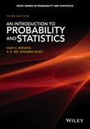
Let (X, Y) be a two-dimensional RV with PMF
Then
and

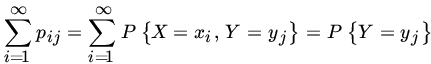
Let us write
Then ![]() and
and ![]() ,
, ![]() and
and ![]() , and {pi·}, {pj·} represent PMFs.
, and {pi·}, {pj·} represent PMFs.
If (X, Y) is an RV of the continuous type with PDF f, then

and

satisfy ![]() , and
, and  ,
,  . It follows that f1(x) and f2(y) are PDFs.

Fig. 4  .
.
In general, given a DF F(x1, x2, …, xn) of an n-dimensional RV (X1, X2, …, Xn), one can obtain any k-dimensional ![]() marginal DF from it. Thus the marginal DF of (Xi1, Xi2, …, Xik), where
marginal DF from it. Thus the marginal DF of (Xi1, Xi2, …, Xik), where ![]() , is given by
, is given by

We now consider the concept of conditional distributions. Let (X, Y) be an RV of the discrete type with PMF ![]() . The marginal PMFs are
. The marginal PMFs are ![]() Recall that, if
Recall that, if ![]() and
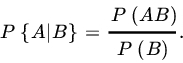
and ![]() , the conditional probability of A, given B, is defined by
, the conditional probability of A, given B, is defined by
Take ![]() and
and ![]() , and assume that
, and assume that ![]() Then
Then ![]() and
and

For fixed j, the function ![]() and
and ![]() Thus
Thus ![]() , for fixed j, defines a PMF.
, for fixed j, defines a PMF.
Next suppose that (X, Y) is an RV of the continuous type with joint PDF f. Since ![]() for any x,y, the probability
for any x,y, the probability ![]() or
or ![]() is not defined. Let
is not defined. Let ![]() , and suppose that
, and suppose that ![]() . For every x and every interval
. For every x and every interval ![]() , consider the conditional probability of the event
, consider the conditional probability of the event ![]() , given that
, given that ![]() . We have
. We have

For any fixed interval ![]() , the above expression defines the conditional DF of X, given that
, the above expression defines the conditional DF of X, given that ![]() , provided that
, provided that ![]() . We shall be interested in the case where the limit
. We shall be interested in the case where the limit
exists.
Suppose that (X, Y) is an RV of the continuous type with PDF f. At every point (x, y) where f is continuous and the marginal PDF ![]() and is continuous, we have
and is continuous, we have

Dividing numerator and denominator by 2ε and passing to the limit as ![]() , we have
, we have

It follows that there exists a conditional PDF of X, given ![]() , that is expressed by
, that is expressed by

We have thus proved the following theorem.
It is clear that similar definitions may be made for the conditional DF and conditional PDF of the RV Y, given X = x, and an analog of Theorem 6 holds.
In the general case, let (X1, X2, …, Xn) be an n-dimensional RV of the continuous type with PDF ![]() . Also, let {i1 < i2 <
. Also, let {i1 < i2 < ![]() < ik, j1 < j2 <
< ik, j1 < j2 < ![]() < jl} be a subset of {1, 2, …, n}. Then
< jl} be a subset of {1, 2, …, n}. Then

provided that the denominator exceeds 0. Here ![]() is the joint marginal PDF of
is the joint marginal PDF of ![]() . The conditional densities are obtained in a similar manner.
. The conditional densities are obtained in a similar manner.
The case in which (X1, X2, … , Xn) is of the discrete type is similarly treated.
We conclude this section with a discussion of a technique called truncation. We consider two types of truncation each with a different objective. In probabilistic modeling we use truncated distributions when sampling from an incomplete population.
If X is a discrete RV with PMF ![]() , the truncated distribution of X is given by
, the truncated distribution of X is given by

If X is of the continuous type with PDF f, then

The PDF of the truncated distribution is given by

Here T is not necessarily a bounded set of real numbers. If we write Y for the RV with distribution function ![]() , then Y has support T.
, then Y has support T.
The second type of truncation is very useful in probability limit theory specially when the DF F in question does not have a finite mean. Let ![]() be finite real numbers. Define RV X* by
be finite real numbers. Define RV X* by
This method produces an RV for which ![]() so that X* has moments of all orders. The special case when
so that X* has moments of all orders. The special case when ![]() and
and ![]() is quite useful in probability limit theory when we wish to approximate X through bounded rvs. We say that Xc is X truncated at c if
is quite useful in probability limit theory when we wish to approximate X through bounded rvs. We say that Xc is X truncated at c if ![]() for
for ![]() . Then
. Then ![]() . Moreover,
. Moreover,
so that c can be selected sufficiently large to make ![]() arbitrarily small. For example, if
arbitrarily small. For example, if ![]() then
then
and given ![]() , we can choose c such that
, we can choose c such that ![]() .
.
The distribution of Xc is no longer the truncated distribution ![]() . In fact,
. In fact,

where F is the DF of X and Fc, that of Xc.
A third type of truncation, sometimes called Winsorization, sets
This method also produces an RV for which ![]() , moments of all orders for X* exist but its DF is given by
, moments of all orders for X* exist but its DF is given by
PROBLEMS 4.2
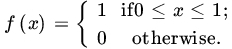
- Let
 if
if  , if
, if  . Does F define a DF in the plane?
 - Let T be a closed triangle in the plane with vertices
 , and
, and  . Let F(x,y) denote the elementary area of the intersection of T with
  . Show that F defines a DF in the plane, and find its marginal DFs.
 - Let (X, Y) have the joint PDF f defined by
 inside the square with corners at the points (1,0), (0,1), (−1,0), and (0, −1) in the (x,y)-plane, and = 0 otherwise. Find the marginal PDFs of X and Y and the two conditional PDFs.
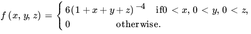
 - Let
 otherwise, be the joint PDF of (X, Y, Z). Compute
  and P{X = Y < Z}.
 - Let (X, Y) have the joint PDF
 , and = 0 otherwise. Find
  .
. - For DFs F, F1, F2,…,Fn show that

for all real numbers x1,x2,…,xn if and only if Fi,’s are marginal DFs of F.
- For the bivariate negative binomial distribution

where
 is an integer,
  , find the marginal PMFs of X and Y and the conditional distributions.
In Problems 8−10 the bivariate distributions considered are not unique generalizations of the corresponding univariate distributions.
- For the bivariate Cauchy RV (X, Y) with PDF

find the marginal PDFs of X and Y. Find the conditional PDF of Y given
 .
.
- For the bivariate beta RV (X, Y) with PDF

where p1 , p2, p3 are positive real numbers, find the marginal PDFs of X and Y and the conditional PDFs. Find also the conditional PDF of
 , given X = x.
 - For the bivariate gamma RV (X, Y) with PDF

find the marginal PDFs of X and Y and the conditional PDFs. Also, find the conditional PDF of
 , given
  , and the conditional distribution of X/Y, given
  .
. - For the bivariate hypergeometric RV (X, Y) with PMF

where
 , N,n integers with
  , and
, and  so that
  , find the marginal PMFs of X and Y and the conditional PMFs.
 - Let X be an RV with PDF
 if
if  , and = 0 otherwise. Let
  . Find the PDF of the truncated distribution of X, its means, and its variance.
 - Let X be an RV with PMF

Suppose that the value
 cannot be observed. Find the PMF of the truncated RV, its mean, and its variance.
 - Is the function

a joint density function? If so, find
 , where (X, Y, Z, U) is a random variable with density f.
 - Show that the function defined by

and 0 elsewhere is a joint density function.
- Find
 .
. - Find
 .
.
- Find
- Let (X, Y) have joint density function f and joint distribution function F. Suppose that

holds for
 and
and  . Show that
- Suppose (X, Y, Z) are jointly distributed with density

Find
 . Hence find the probability that
  . (Here g is density function on
  .)
.)
4.3 INDEPENDENT RANDOM VARIABLES
We recall that the joint distribution of a multiple RV uniquely determines the marginal distributions of the component random variables, but, in general, knowledge of marginal distributions is not enough to determine the joint distribution. Indeed, it is quite possible to have an infinite collection of joint densities fα with given marginal densities.
In this section we deal with a very special class of distributions in which the marginal distributions uniquely determine the joint distribution of a multiple RV. First we consider the bivariate case.
Let F(x, y) and F1(x), F2(y), respectively, be the joint DF of (X, Y) and the marginal DFs of X and Y.
Note that Φ(X2) and ψ(Y2) are independent where Φ and ψ are Borel–measurable functions. But X is not a Borel-measurable function of X2.
It is clear that an analog of Theorem 1 holds, but we leave the reader to construct it.
The following result is easy to prove.
Remark 1. It is quite possible for RVs X1, X2,…Xn to be pairwise independent without being mutually independent. Let (X, Y, Z) have the joint PMF defined by

Clearly, X, Y, Z are not independent (why?). We have

It follows that X and Y, Y and Z, and X and Z are pairwise independent.
Similarly, one can speak of an independent family of RVs.
According to Definition 4, X and Y are identically distributed if and only if they have the same distribution. It does not follow that ![]() with probability 1 (see Problem 7). If
with probability 1 (see Problem 7). If ![]() , we say that X and Y are equivalent RVs. All Definition 4 says is that X and Y are identically distributed if and only if
, we say that X and Y are equivalent RVs. All Definition 4 says is that X and Y are identically distributed if and only if
Nothing is said about the equality of events ![]() and
and ![]() .
.
Of course, the independence of (X1, X2,… ,Xm) and (Y1, Y2,… ,Yn) does not imply the independence of components X1, X2,… ,Xm of X or components Y1, Y2,… ,Yn of Y.
Remark 2. It is possible that an RV X may be independent of Y and also of Z, but X may not be independent of the random vector (Y,Z). See the example in Remark 1.
Let X1, X2,… ,Xn be independent and identically distributed RVs with common DF F. Then the joint DF G of (X1,X2,… ,Xn) is given by

We note that for any of the n! permutations ![]() of (x1, x2,…,xn)
of (x1, x2,…,xn)

so that G is a symmetric function of x1, x2,… ,xn. Thus ![]() , where
, where ![]() means that X and Y are identically distributed RVs.
means that X and Y are identically distributed RVs.
Clearly if X1, X2,…, Xn are exchangeable, then Xi are identically distributed but not necessarily independent.
In view of Theorem 6, Xs is symmetric about 0 so that
If ![]() ,then
,then ![]() , and EXs = 0.
, and EXs = 0.
The technique of symmetrization is an important tool in the study of probability limit theorems. We will need the following result later. The proof is left to the reader.
PROBLEMS 4.3
- Let A be a set of k numbers, and Ω be the set of all ordered samples of size n from A with replacement. Also, let
 be the set of all subsets of Ω, and P be a probability defined on . Let X1, X2,…, Xn be RVs defined on (Ω, , P) by setting

Show that X1, X2,… ,Xn are independent if and only if each sample point is equally likely.
- Let X1, X2 be iid RVs with common PMF

Write
 . Show that X1, X2, X3 are pairwise independent but not independent.
 - Let (X1, X2, X3) be an RV with joint PMF

where

Are X1,X2,X3 independent? Are X1,X2,X3 pairwise independent? Are
 and X3 independent?
No; Yes; No.
- Let X and Y be independent RVs such that XY is degenerate at
 . That is,
  . Show that X and Y are also degenerate.
 - Let (Ω, , P) be a probability space and A, B ∈ . Define X and Y so that

Show that X and Y are independent if and only if A and B are independent.
- Let X1,X2,… ,Xn be a set of exchangeable RVs. Then

- Let X and Y be identically distributed. Construct an example to show that X and Y need not be equal, that is,
 need not equal 1.
 - Prove Lemma 1.
- Let X1,X2,… ,Xn be RVs with joint PDF f, and let fj be the marginal PDF of
 . Show that X1, X2,… ,Xn are independent if and only if

- Suppose two buses, A and B, operate on a route. A person arrives at a certain bus stop on this route at time 0. Let X and Y be the arrival times of buses A and B, respectively, at this bus stop. Suppose X and Y are independent and have density functions given, respectively, by

What is the probability that bus A will arrive before bus B?
- Consider two batteries, one of Brand A and the other of Brand B. Brand A batteries have a length of life with density function

whereas Brand B batteries have a length of life with density function given by

Brand A and Brand B batteries operate independently and are put to a test. What is the probability that Brand B battery will outlast Brand A? In particular, what is the probability if
 ?
? -
- Let (X, Y) have joint density f. Show that X and Y are independent if and only if for some constant
 and nonnegative functions f1 and f2
for all
and nonnegative functions f1 and f2
for all
 .
. - Let
 , and fX, fY are marginal densities of X and Y, respectively. Show that if X and Y are independent then
  .
.
- Let (X, Y) have joint density f. Show that X and Y are independent if and only if for some constant
- If Φ is the CF of X, show that the CF of Xs is real and even.
- Let X, Y be jointly distributed with PDF
 otherwise. Show that
  and
and  has a symmetric distribution.
4.4 FUNCTIONS OF SEVERAL RANDOM VARIABLES
Let X1, X2,… ,Xn be RVs defined on a probability space (Ω, ![]() , P). In practice we deal with functions of X1, X2,… , Xn such as
, P). In practice we deal with functions of X1, X2,… , Xn such as ![]() , min (X1,… ,Xn), and so on. Are these also RVs? If so, how do we compute their distribution given the joint distribution of X1, X2 …, Xn?
, min (X1,… ,Xn), and so on. Are these also RVs? If so, how do we compute their distribution given the joint distribution of X1, X2 …, Xn?
What functions of (X1, X2,… ,Xn) are RVs?
In particular, if g: ![]() is a continuous function, then g(X1,X2,… ,Xn) is an RV.
is a continuous function, then g(X1,X2,… ,Xn) is an RV.
How do we compute the distribution of g(X1,X2,… ,Xn)? There are several ways to go about it. We first consider the method of distribution functions. Suppose that ![]() is real-valued, and let
is real-valued, and let ![]() . Then
. Then

where in the continuous case f is the joint PDF of (X1,…, Xn).
In the continuous case we can obtain the PDF of ![]() by differentiating the DF
by differentiating the DF ![]() with respect to y provided that Y is also of the continuous type. In the discrete case it is easier to compute
with respect to y provided that Y is also of the continuous type. In the discrete case it is easier to compute ![]() .
.
We take a few examples,


Fig. 1 (a)  and (b)
  .
.
There are two cases to consider according to whether ![]() or
or ![]() (Fig. 1a and 1b). In the former case,
(Fig. 1a and 1b). In the former case,

and in the latter case,

Hence the density function of Y is given by
The method of distribution functions can also be used in the case when g takes values in ![]() m, 1 ≤ m ≤ n, but the integration becomes more involved.
m, 1 ≤ m ≤ n, but the integration becomes more involved.
Let ![]() and
and ![]() . Then the joint distribution of (Y1, Y2) is given by
. Then the joint distribution of (Y1, Y2) is given by
where ![]() Clearly,
Clearly, ![]() so that the set A is as shown in Fig. 2. It follows that
so that the set A is as shown in Fig. 2. It follows that

Fig. 2  .
.
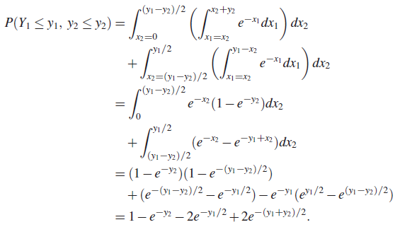
Hence the joint density of Y1, Y2 is given by

The marginal densities of Y1, Y2 are easily obtained as

We next consider the method of transformations. Let (X1,…, Xn) be jointly distributed with continuous PDF f(x1, x2,…,xn), and let ![]() , where
, where
be a mapping of ![]() n to Rn. Then
n to Rn. Then
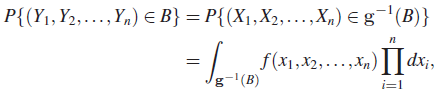
where ![]() . Let us choose B to be the n-dimensional interval
. Let us choose B to be the n-dimensional interval
Then the joint DF of Y is given by

and (if GY is absolutely continuous) the PDF of Y is given by
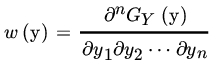
at every continuity point y of w. Under certain conditions it is possible to write w in terms of f by making a change of variable in the multiple integral.
Then (Y1, Y2,… ,Yn) has a joint absolutely continuous DF with PDF given by
Proof. For (y1, y2,…,yn) ∈ ![]() n, let
n, let
Then
and

Result (1) now follows on differentiation of DF GY.
Remark 1. In actual applications we will not know the mapping from x1, x2,…,xn to y1, y2,…,yn completely, but one or more of the functions gi will be known. If only ![]() , of the gi’s are known, we introduce arbitrarily
, of the gi’s are known, we introduce arbitrarily ![]() functions such that the conditions of the theorem are satisfied. To find the joint marginal density of these k variables we simply integrate the w function over all the
functions such that the conditions of the theorem are satisfied. To find the joint marginal density of these k variables we simply integrate the w function over all the ![]() variables that were arbitrarily introduced.
variables that were arbitrarily introduced.
Remark 2. An analog of Theorem 2.5.4 holds, which we state without proof.
Let ![]() be an RV of the continuous type with joint PDF f, and let
be an RV of the continuous type with joint PDF f, and let ![]() , be a mapping of
, be a mapping of ![]() n into itself. Suppose that for each y the transformation g has a finite number
n into itself. Suppose that for each y the transformation g has a finite number ![]() of inverses. Suppose further that
of inverses. Suppose further that ![]() n can be partitioned into k disjoint sets A1, A2,… ,Ak, such that the transformation g from
n can be partitioned into k disjoint sets A1, A2,… ,Ak, such that the transformation g from ![]() into
into ![]() n is one-to-one with inverse transformation
n is one-to-one with inverse transformation
Suppose that the first partial derivatives are continuous and that each Jacobian

is different from 0 in the range of the transformation. Then the joint PDF of Y is given by

Fig. 3  .
.
In Example 6 the transformation used is orthogonal and is known as Helmert’s transformation. In fact, we will show in Section 6.5 that under orthogonal transformations iid RVs with PDF f defined above are transformed into iid RVs with the same PDF.
It is easily verified that

We have therefore proved that ![]() is independent of
is independent of ![]() This is a very important result in mathematical statistics, and we will return to it in Section 7.7.
This is a very important result in mathematical statistics, and we will return to it in Section 7.7.
An important application of the result in Remark 2 will appear in Theorem 4.7.2.
Finally, we consider a technique based on MGF or CF which can be used in certain situations to determine the distribution of a function g(X1, X2,… ,Xn) of X1, X2,… ,Xn.
Let (X1, X2,… ,Xn) be an n-variate RV, and g be a Borel-measurable function from ![]() n to
n to ![]() 1.
1.
Let ![]() , and let h(y) be its PDF. If
, and let h(y) be its PDF. If ![]() then
then

An analog of Theorem 3.2.1 holds. That is,

in the sense that if either integral exists so does the other and the two are equal. The result also holds in the discrete case.
Some special functions of interest are ![]() , where k1, k2,… ,kn are non-negative integers,
, where k1, k2,… ,kn are non-negative integers, ![]() , where t1,t2,… ,tn are real numbers, and
, where t1,t2,… ,tn are real numbers, and ![]() , where
, where ![]() .
.
We will mostly deal with MGF even though the condition that it exist for ![]() restricts its application considerably. The multivariate MGF (CF) has properties similar to the univariate MGF discussed earlier. We state some of these without proof. For notational convenience we restrict ourselves to the bivariate case.
restricts its application considerably. The multivariate MGF (CF) has properties similar to the univariate MGF discussed earlier. We state some of these without proof. For notational convenience we restrict ourselves to the bivariate case.
A formal definition of moments in the multivariate case will be given in Section 4.5.
The MGF technique uses the uniqueness property of Theorem 4. In order to find the distribution (DF, PDF, or PMF) of ![]() we compute the MGF of Y using definition. If this MGF is one of the known kind then Y must have this kind of distribution. Although the technique applies to the case when Y is an m-dimensional RV,
we compute the MGF of Y using definition. If this MGF is one of the known kind then Y must have this kind of distribution. Although the technique applies to the case when Y is an m-dimensional RV, ![]() , we will mostly use it for the
, we will mostly use it for the ![]() case.
case.
The following result has many applications as we will see. Example 9 is a special case.
From these examples it is clear that to use this technique effectively one must be able to recognize the MGF of the function under consideration. In Chapter 5 we will study a number of commonly occurring probability distributions and derive their MGFs (whenever they exist). We will have occasion to use Theorem 7 quite frequently.
For integer-valued RVs one can sometimes use PGFs to compute the distribution of certain functions of a multiple RV.
We emphasize the fact that a CF always exists and analogs of Theorems 4–7 can be stated in terms of CFs.
PROBLEMS 4.4
- Let F be a DF and ε be a positive real number. Show that

and

are also distribution functions.
- Let X, Y be iid RVs with common PDF

- Find the PDF of RVs
 , X – Y, XY, X/Y, min{X, Y}, max{X, Y}, min{X, Y}/max{X, Y}, and
- Let
 and
and  . Find the conditional PDF of V, given
  , for some fixed
  .
. - Show that U and
 are independent.
- Find the PDF of RVs
- Let X and Y be independent RVs defined on the space (Ω, , P). Let X be uniformly distributed on (–a, a),
 , and Y be an RV of the continuous type with density f, where f is continuous and positive on . Let F be the DF of Y. If u0 ∈ (–a, a) is a fixed number, show that

where
 is the conditional density function of Y, given.
  .
. - Let X and Y be iid RVs with common PDF

Find the PDFs of RVs XY, X/Y, min {X, Y}, max {X, Y}, min {X, Y}/max {X, Y}.
- Let X1, X2, X3 be iid RVs with common density function
Show that the PDF of
 is given by
An extension to the n-variate case holds.
- Let X and Y be independent RVs with common geometric PMF

Also, let
 . Find the joint distribution of M and X, the marginal distribution of M, and the conditional distribution of X, given M.
 - Let X be a nonnegative RV of the continuous type. The integral part, Y, of X is distributed with PMF
 ; and the fractional part, Z, of X has PDF,
  if
if  , and = 0 otherwise. Find the PDF of X, assuming that Y and Z are independent.
 - Let X and Y be independent RVs. If at least one of X and Y is of the continuous type, show that
 is also continuous. What if X and Y are not independent?
 - Let X and Y be independent integral RVs. Show that
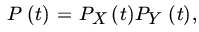
where P, PX, and PY, respectively, are the PGFs of
 , X, and Y.
 - Let X and Y be independent nonnegative RVs of the continuous type with PDFs f and g, respectively. Let
 , and
, and  if
if  and let g be arbitrary. Show that the MGF M (t) of Y, which is assumed to exist, has the property that the DF of X/Y is
  .
. - Let X, Y, Z have the joint PDF
Find the PDF of
 .
. .
. - Let X and Y be iid RVs with common PDF

Find the PDF of
 .
. - Let X and Y be iid RVs with common PDF f defined in Example 8. Find the joint PDF of U and V in the following cases:
 ,
,  ,
, 
 ,
, 
- Construct an example to show that even when the MGF of
 can be written as a product of the MGF of X and the MGF of Y, X and Y need not be independent.
 - Let X1, X2,…, Xn be iid with common PDF

Using the distribution function technique show that
- The joint PDF of
 , and
, and  is given by
and = 0 otherwise.
is given by
and = 0 otherwise.
- The PDF of X(n) is given by
and that of X(1) by


- The joint PDF of
- Let X1, X2 be iid with common Poisson PMF

where
 is a constant. Let
  and
and  . Find the PMF of X(2).
 - Let X have the binomial PMF

Let Y be independent of X and
 . Find PMF OF
  and
and  .
.
4.5 COVARIANCE, CORRELATION AND MOMENTS
Let X and Y be jointly distributed on (Ω, ![]() , P). In Section 4.4 we defined Eg (X, Y) for Borel functions g on
, P). In Section 4.4 we defined Eg (X, Y) for Borel functions g on ![]() 2. Functions of the form
2. Functions of the form ![]() where j and k are nonnegative integers are of interest in probability and statistics.
where j and k are nonnegative integers are of interest in probability and statistics.
Recall (Theorem 3.2.8) that ![]() is minimized when we choose
is minimized when we choose ![]() so that EY may be interpreted as the best constant predictor of Y. If instead, we choose to predict Y by a linear function of X, say
so that EY may be interpreted as the best constant predictor of Y. If instead, we choose to predict Y by a linear function of X, say ![]() , and measure the error in this prediction by
, and measure the error in this prediction by ![]() , then we should choose a and b to minimize this so-called mean square error. Clearly,
, then we should choose a and b to minimize this so-called mean square error. Clearly, ![]() is minimized, for any a, by choosing
is minimized, for any a, by choosing ![]() . With this choice of b, we find a such that
. With this choice of b, we find a such that

is minimum. An easy computation shows that the minimum occurs if we choose

Provided ![]() . Moreover,
. Moreover,

Let us write
Then (8) shows that predicting Y by a linear function of X reduces the prediction error from ![]() to
to ![]() . We may therefore think of ρ as a measure of the linear dependence between RVs X and Y.
. We may therefore think of ρ as a measure of the linear dependence between RVs X and Y.
If X and Y are independent, then from (5) ![]() , and X and Y are uncorrelated. If, however,
, and X and Y are uncorrelated. If, however, ![]() then X and Y may not necessarily be independent.
then X and Y may not necessarily be independent.
Let us now study some properties of the correlation coefficient. From the definition we see that ρ (and also cov (X, Y)) is symmetric in X and Y.
Equality in (11) holds if and only if ![]() , or equivalently,
, or equivalently, ![]() holds. This implies and is implied by
holds. This implies and is implied by ![]() . Here a ≠ 0.
. Here a ≠ 0.
Remark 1. From (7) and (9) we note that the signs of a and ρ are the same so if ![]() then
then ![]() where a > 0, and if
where a > 0, and if ![]() then
then ![]() .
.
The existence of ES follows easily by replacing each aj by |aj| and each xij by |xij| and remembering that ![]() . The case of continuous type (X1, X2,…,Xn) is similarly treated.
. The case of continuous type (X1, X2,…,Xn) is similarly treated.
Let X and Y be independent, and g1 (∙) and g2 (∙) be Borel-measurable functions. Then we know (Theorem 4.3.3) that g1 (X) and g2 (Y) are independent. If E{g1(X)}, E{g2(Y)}, and E{g1 (X)g2(Y)} exist, it follows from Theorem 4 that
Conversely, if for any Borel sets A1 and A2 we take ![]() if X ∈ A1, and = 0 otherwise, and
if X ∈ A1, and = 0 otherwise, and ![]() if
if ![]() , and = 0 otherwise, then
, and = 0 otherwise, then
and ![]() ,
, ![]() Relation (14) implies that for any Borel sets A1 and A2 of real numbers
Relation (14) implies that for any Borel sets A1 and A2 of real numbers
It follows that X and Y are independent if (14) holds. We have thus proved the following theorem.
Note that the result holds if we replace independence by the condition that Xi’s are exchangeable and uncorrelated.
We conclude this section with some important moment inequalities. We begin with the simple inequality
where ![]() for
for ![]() and
and ![]() for r > 1. For
for r > 1. For ![]() and
and ![]() , (20) is trivially true.
, (20) is trivially true.
First note that it is sufficient to prove (20) when ![]() . Let
. Let ![]() , and write
, and write ![]() . Then
. Then
Writing ![]() , we see that
, we see that
where ![]() . It follows that.
. It follows that. ![]() , and < 0 if r < 1. Thus
, and < 0 if r < 1. Thus
while
Note that ![]() is trivially true since
is trivially true since
![]() An immediate application of (20) is the following result.
An immediate application of (20) is the following result.
Corollary. Taking ![]() , we obtain the Cauchy–Schwarz inequality,
, we obtain the Cauchy–Schwarz inequality,
The final result of this section is an inequality due to Minkowski.
PROBLEMS 4.5
- Suppose that the RV (X, Y) is uniformly distributed over the region
 Find the covariance between X and Y.
 - Let (X, Y) have the joint PDF given by

Find all moments of order 2.
- Let (X, Y) be distributed with joint density
Find the MGF of (X, Y). Are X, Y independent? If not, find the covariance between X and Y.
 dependent.
 - For a positive RV X with finite first moment show that (1)
 and (2)
  .
. - If X is a nondegenerate RV with finite expectation and such that
 , then

(Kruskal [56])
- Show that for


and hence that

- Given a PDF f that is nondecreasing in the interval
 , show that for any s>0

with the inequality reversed if f is nonincreasing.
- Derive the Lyapunov inequality (Theorem 3.4.3)

from Hölder’s inequality (22).
- Let X be an RV with
 for
for  . Show that the function log E|X|r is a convex function of r.
 - Show with the help of an example that Theorem 9 is not true for

- Show that the converse of Theorem 8 also holds for independent RVs, that is, if
 for some
  and X and Y are independent, then
  .
.
[Hint: Without loss of generality assume that the median of both X and Y is 0. Show that, for any
 ,
,  . Now use the remarks preceding Lemma 3.2.2 to conclude that
  .]
.] - Let (Ω, , P) be a probability space, and A1, A2,…,An be events in such that
 . Show that

(Chung and Erdös [14])
[Hint: Let Xk be the indicator function of Ak,
 . Use the Cauchy–Schwarz inequality.]
 - Let (Ω, , P) be a probability space, and A,B, ∈ with
 ,
,  . Define ρ(A, B) by ρ(A, B) = correlation coefficient between RVs IA, and IB, where IA, IB, are the indicator functions of A and B, respectively. Express ρ(A, B) in terms of PA, PB, and P(AB) and conclude that
  if and only if A and B are independent. What happens if
  or if
or if  ?
?
- Show that
and


- Show that

- Show that
- Let X1, X2,…,Xn be iid RVs and define

Suppose that the common distribution is symmetric. Assuming the existence of moments of appropriate order, show that
 .
. - Let X,Y be iid RVs with common standard normal density

Let
 and
and  . Find the MGF of the rendom variable (U, V). Also, find the correlation coefficient between U and V. Are U and V independent?
 - Let X and Y be two discrete RVs:

and

Show that X and Y are independent if and only if the correlation coefficient between X and Y is 0.
- Let X and Y be dependent RVs with common means 0, variance 1, and correlation coefficient ρ. Show that

- Let X1, X2 be independent normal RVs with density functions

Also let

Find the correlation coefficient between Z and W and show that

where ρ denotes the correlation coefficient between Z and W.
- Let (X1, X2,…,Xn) be an RV such that the correlation coefficient between each pair Xi, Xj,
 , is ρ. Show that
  .
. - Let X1, X2,…,Xm+n be iid RVs with finite second moment. Let
 . Find the correlation coefficient between Sn and
  , where
  .
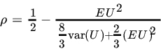
. - Let f be the PDF of a positive RV, and write
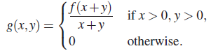
Show that g is a density function in the plane. If the mth moment of f exists for some positive integer m, find EXm. Compute the means and variances of X and Y and the correlation coefficient between X and Y in terms of moments of f. (Adapted from Feller [26, p. 100].)
If U has PDF f, then
 for
for  ;
;  .
. - A die is thrown
 times. After each throw a + sign is recorded for 4, 5, or 6, and a – sign for 1, 2, or 3, the signs forming an ordered sequence. Each sign, except the first and the last, is attached to a characteristic RV that assumes the value 1 if both the neighboring signs differ from the one between them and 0 otherwise. Let X1,X2,…,Xn be these characteristic RVs, where Xi corresponds to the
  st sign (i = 1, 2,…,n) in the sequence. Show that

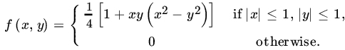
- Let (X, Y) be jointly distributed with PDF f defined by
 inside the square with corners at the points (0, 1), (1, 0), (–1, 0), (0,–1) in the (x, y)-plane, and
  otherwise. Are X, Y independent? Are they uncorrelated?
4.6 CONDITIONAL EXPECTATION
In Section 4.2 we defined the conditional distribution of an RV X, given Y. We showed that, if (X, Y) is of the discrete type, the conditional PMF of X, given ![]() , where
, where ![]() , is a PMF when considered as a function of the xi’s (for fixed yj). Similarly, if (X, Y) is an RV of the continuous type with PDF f (x,y) and marginal densitiesf1 and f2, respectively, then, at every point (x, y) at which f is continuous and at which
, is a PMF when considered as a function of the xi’s (for fixed yj). Similarly, if (X, Y) is an RV of the continuous type with PDF f (x,y) and marginal densitiesf1 and f2, respectively, then, at every point (x, y) at which f is continuous and at which ![]() and is continuous, a conditional density function of X, given Y, exists and may be defined by
and is continuous, a conditional density function of X, given Y, exists and may be defined by

We also showed that ![]() , for fixed y, when considered as a function of x is a PDF in its own right. Therefore, we can (and do) consider the moments of this conditional distribution.
, for fixed y, when considered as a function of x is a PDF in its own right. Therefore, we can (and do) consider the moments of this conditional distribution.
Needless to say, a similar definition may be given for the conditional expectation ![]() .
.
It is immediate that ![]() satisfies the usual properties of an expectation provided we remember that
satisfies the usual properties of an expectation provided we remember that ![]() is not a constant but an RV. The following results are easy to prove. We assume existence of indicated expectations.
is not a constant but an RV. The following results are easy to prove. We assume existence of indicated expectations.
for any Borel functions g1, g2.
The statements in (3), (4), and (5) should be understood to hold with probability 1.
for independent RVs X and Y.
If ϕ(X, Y) is a function of X and Y, then
for any Borel functions ψ and Φ.
Again (8) should be understood as holding with probability 1. Relation (7) is useful as a computational device. See Example 3 below.
The moments of a conditional distribution are defined in the usual manner. Thus, for ![]() ,
, ![]() defines the rth moment of the conditional distribution. We can define the central moments of the conditional distribution and, in particular, the variance. There is no difficulty in generalizing these concepts for n-dimensional distributions when
defines the rth moment of the conditional distribution. We can define the central moments of the conditional distribution and, in particular, the variance. There is no difficulty in generalizing these concepts for n-dimensional distributions when ![]() . We leave the reader to furnish the details.
. We leave the reader to furnish the details.
Theorem 1 is quite useful in computation of Eh(X) in many applications.
Equation (11) follows immediately from (10). The equality in (11) holds if and only if
which holds if and only if with probability 1
PROBLEMS 4.6
- Let X be and RV with PDF given by

Find
 , where a and b are constants.
 where Φ is the standard normal DF.
 -
- Let (X, Y) be jointly distributed with density
Find E{Y | X}.

- Do the same for the joint density

- Let (X, Y) be jointly distributed with density
- Let (X, Y) be jointly distributed with bivariate normal density

Find
 and
and  . (Here,
  , and
, and  .)
.) - Find
 .
. - Show that
 is minimized by choosing
  .
. - Let X have PMF
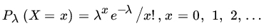
and suppose that λ is a realization of a RV Λ with PDF

Find
 .
. - Find E(XY) by conditioning on X or Y for the following cases:
 .
. .
.
- Suppose X has uniform PDF
 ,
,  and 0 otherwise Let Y be chosen from interval (0, X] according to PDF

Find
 and EYk for any fixed constant
  .
.
4.7 ORDER STATISTICS AND THEIR DISTRIBUTIONS
Let (X1, X2,… ,Xn) be an n-dimensional random variable and (x1, x2,… ,xn) be an n-tuple assumed by (X1, X2,… ,Xn). Arrange (x1, x2,… ,xn) in increasing order of magnitude so that
where ![]() , x(2) is the second smallest value in x1, x2,… ,xn, and so on,
, x(2) is the second smallest value in x1, x2,… ,xn, and so on, ![]() . If any two xi, xj are equal, their order does not matter.
. If any two xi, xj are equal, their order does not matter.
Statistical considerations such as sufficiency, completeness, invariance, and ancillarity (Chapter 8) lead to the consideration of order statistics in problems of statistical inference. Order statistics are particularly useful in nonparametric statistics (Chapter 13) where, for example, many test procedures are based on ranks of observations. Many of these methods require the distribution of the ordered observations which we now study.
In the following we assume that X1, X2,… , Xn are iid RVs. In the discrete case there is no magic formula to compute the distribution of any X(j) or any of the joint distributions. A direct computation is the best course of action.
In the following we assume that X1, X2 ,… ,Xn are iid RVs of the continuous type with PDF f. Let {X(1), X(2),… ,X(n)} be the set of order statistics for X1, X2 ,… ,Xn. Since the Xi are all continuous type RVs, it follows with probability 1 that
It follows (see Remark 2) that

The procedure for computing the marginal PDF of X(r), the rth-order statistic of X1, X2,… ,Xn is similar. The following theorem summarizes the result.
We now compute the joint PDF of X(j) and X(k) ![]() .
.
In a similar manner we can show that the joint PDF of ![]() , is given by
, is given by

for y1 < y2 < ![]() <yk, and = 0 otherwise.
<yk, and = 0 otherwise.
The joint PDF of X(1) and X(n) is given by
and that of the range ![]() by
by
Finally, we consider the moments, namely, the means, variances, and covariances of order statistics. Suppose X1, X2,…Xn are iid RVs with common DF F. Let g be a Borel function on ![]() such that
such that ![]() , where X has DF F. Then for
, where X has DF F. Then for ![]()
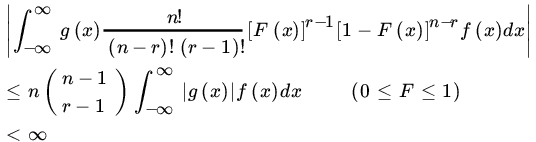
and we write

for ![]() . The converse also holds. Suppose
. The converse also holds. Suppose ![]() for
for ![]() . Then,
. Then,

for ![]() and hence
and hence

Moreover, it also follows that

As a consequence of the above remarks we note that if ![]() for some r,
for some r, ![]() , then
, then ![]() and conversely, if
and conversely, if ![]() for some r,
for some r, ![]() .
.
PROBLEMS 4.7
- Let X(1), X(2),…X(n) be the set of order statistics of independent RVs X1, X2,…,Xn with common PDF

- Show that X(r) and X(s) – X(r) are independent for any
 .
. - Find the PDF of
 .
. - Let
 . Show that (Z1, Z2,…,Zn) and (X1, X2,…,Xn) are identically distributed.
- Show that X(r) and X(s) – X(r) are independent for any
- Let X1, X2,…Xn be iid from PMF

Find the marginal distributions of X(1), X(n), and their joint PMF.
- Let X1, X2,…,Xn be iid with a DF

Show that X(i)/X(n),
 , and X(n) are independent.
 - Let X1, X2,…,Xn be iid RVs with common Pareto DF
 ,
,  where
where  ,
,  Show that
- X(1), (X(2)/X(1), …, X(n)/X(1)) are independent,
- X(1) has Pareto (σ, nα) distribution, and
 has PDF

- Let X1, X2,…,Xn be iid nonnegative RVs of the continuous type. If
 , show that
  . Write
  . Show that

Find EMn in each of the following cases:
- Xi have the common DF

- Xi have the common DF
- Xi have the common DF
- Let X1, X(2)…,X(n) be that order statistics of n independent RVs X1, X2,…,Xn with common PDF
 if
if  , and = 0 otherwise. Show that
  , and
, and  are independent. Find the PDf of Y1, Y2,…,Yn.
 - For the PDF in Problem 4 find EX(r).
- An urn contains N identical marbles numbered 1 through N. From the urn n marbles are drawn and let X(n) be the largest number drawn. Show that
 , and
, and  .
.